Article

Impact of Non-Uniform Irradiance and Temperature Distribution on the Performance of Photovoltaic Generators

by
Petrakis Thomas
1,
Aphrodite Ktena
1,
Panagiotis Kosmopoulos
2,*,
John Konstantaras
3 and
Michael Vrachopoulos
3
1
General Department, National and Kapodistrian University of Athens, Evripos Campus, 34400 Psachna, Greece
2
Institute for Environmental Research and Sustainable Development of the National Observatory of Athens, 15236 Athens, Greece
3
Renewable Energy Sources Laboratory, General Department of the National and Kapodistrian University of Athens, 34400 Psachna, Greece
*
Author to whom correspondence should be addressed.
Energies 2023, 16(17), 6322; https://doi.org/10.3390/en16176322
Submission received: 9 August 2023 / Revised: 24 August 2023 / Accepted: 28 August 2023 / Published: 31 August 2023
(This article belongs to the Special Issue Advances on Solar Energy Materials and Solar Cells)

Abstract

:
The use of photovoltaic (PV) panels has increased rapidly in the last few years and as a result has become one of the main sources of renewable energy. In this context, it is important to understand in detail how a PV panel reacts to different environmental conditions and how these affect total performance. An experiment has been designed to investigate the performance of a PV panel under various highly non-uniform temperature and irradiance profiles, generated by artificial lighting. Measurements of irradiance and temperature distribution are related to measured I–V curves and used as input to the five-parameter model. The results show the limitations of the model to emulate the PV response under such extreme conditions and provide useful insights about the effect of the temperature profile on the PV performance.

1. Introduction

The increasing demand for energy, coupled with the finite resources of non-renewable fuels like coal, oil, and natural gas, has prompted a global shift towards more sustainable and efficient energy practices. This transition is also driven by the urgent need to reduce carbon dioxide (CO2) emissions and mitigate the impacts of climate change [1]. Renewable energy sources (RES), such as solar, wind, hydrothermal, tidal, and biomass, are regarded as eco-friendly, environmentally sustainable, and practically limitless [2]. Photovoltaics (PV), despite their intermittent operation, remain one of the most competitive choices for higher RES penetration since geothermal is limited in nature. Among these three, solar energy holds the greatest worldwide potential, as geothermal sources are confined to specific locations and the availability of biomass is not universally prevalent in nature [3]. The abundance of solar energy surpasses global energy requirements, and its availability extends, to varying degrees, across every nation on the planet [4]. Converting solar radiation directly into electrical energy eliminates the emission of pollutants during operation, consequently mitigating global warming. The significant decline in PV module costs and the concurrent rise in petrochemical fuel prices have stimulated the widespread adoption of PV systems [5]. The word “photovoltaic” pertains to the process by which solar energy is transformed into electric energy through a solar cell [6]. The solar cell operates on the principle of a p-n semiconductor junction. Its power output is directly proportional to the solar irradiation it receives. Conversely, the power output declines as the temperature of the solar cell increases [7]. The substantial expansion of the PV industry and the proliferation of installed PV systems globally have underscored the requirement for enhanced monitoring and simulation tools. Hence, modeling these systems under diverse operational and meteorological conditions is imperative [5]. The modeling of PV cells and plants is useful both for providing insight and understanding the factors determining and optimizing their output as well as for providing useful tools for their design and optimal control [8]. For the simulation of the operation of specific PV panels, certain features need to be determined through identification techniques utilizing data obtained in the laboratory or supplied by the manufacturer.
A well-known class of models relying on the PV phenomenon and p-n junction models are the single-diode models (SDM), dual-diode models (DDM), and triple-diode models (TDM). They all model the response of the PV cell, which is the building block of a PV panel. They use solar irradiance (in W/m2) and temperature (in K) as inputs and yield the output DC I (in A) under specific loading conditions (in V). Among these, SDM distinguishes itself by its effective performance and uncomplicated nature. It involves a light-dependent DC source to model the p-n junction response, and a single-diode alongside two resistances, one in series ( R s ) and the other in parallel ( R s h ) to model the losses. SDM encapsulates a collective sum of five parameters, namely the photocurrent I L , the diode ideality factor n, the reverse saturation current I 0 and the loss of resistances R s and R s h offering a balance between performance and simplicity. DDM sets itself apart from SDM by introducing a second diode, consequently increasing the parameter count to seven. This increase in the number of parameters enhances the model accuracy, albeit at the cost of greater complexity. TDM is acknowledged as the most intricate model due to its incorporation of triple diodes, which emulate the behaviors of specific cell types. Employing TDM necessitates considerable computational resources to compute a total of nine distinct parameters [8,9]. As already mentioned, the solar cell serves as the fundamental cornerstone of any PV power system. It occupies a relatively small area of a few cm2 and can generate around one watt of power under standard conditions. To attain increased power outputs, tens of these cells are connected series and/or parallel thus constituting a panel whose area is in the order of m2 [10]. For higher power yields, the panels are interconnected both in series and parallel arrangements, forming arrays [11]. PV systems are scalable and have the flexibility to connect to low or medium-voltage distribution networks and they are classified into three primary size categories depending on their installed capacity: small (1 up to 1000 kWp), medium (1 to 100 MWp), and large (above 100 MWp) [12].
It is well established that the performance of PV panels depends on the power density or solar irradiation G and the temperature T on the surface of the panel as well as on the air mass AM traveled by the sunlight through the Earth’s atmosphere [13,14]. Notably, the diode models disregard the impact of AM on their calculations. Recent existing papers in the literature focus on the identification of SDM parameters via software simulation with new improved methods [15,16] via outdoor experiments [4,17,18,19,20,21,22,23] or both [24] in the morning and afternoon which are the hours of the day that PV does not operate under the STC conditions.
The motivation behind the experimental and modeling work presented here is the limitations of the available models to accurately simulate the PV operation under realistic atmospheric conditions. The density of the atmosphere in terms of clouds, aerosols, gases, and relative humidity can introduce large uncertainties to the PV operating conditions in terms of temperature, panel material, dust deposition, shadowing, etc. In this direction, the modeling of PV cells under laboratory-controlled operating conditions, is necessary for further outdoor experiments, especially for distributed PV in energy communities, where the electricity handling entities need precise production level estimations for efficient energy management, planning, and optimization procedures. This study intends to act as a basis for further modeling experiments to unravel the complexity of the atmosphere (e.g., hot spots (see [1,2,3,4,5,6,7,8,9,10,11,12,13] and references therein)) and surface (e.g., at urban environments) where the deployments at rooftop level are highly affected by shadowing effects on PV operation and energy production levels (e.g., using Earth observation data sources and methods) and the real operating conditions using the experimental findings as reference values for precise and reliable model estimations at any solar system scale.
This work presents the performance of the five-parameter PV cell model for various irradiance and temperature combinations against experimental measurements under controlled conditions in the laboratory. An investigation was carried out involving the adjustment of PV panels to varying inclinations ranging from 0 to 9 degrees, while also considering different levels of lighting conditions. Furthermore, a simulation was conducted to establish the basis for comparison. The structure of the paper is as follows: Section 2 describes in detail the methodology and materials used to conduct the experiment and study the PV operation in various irradiance conditions. Section 3 includes the results of irradiance measurements displayed in 3D visualization graphs of the PV module surface for different inclinations and irradiance levels, thermal camera snapshots of the PV surface under exposure to artificial lighting, I-V, and P-V curves, both measured and simulated. The results are discussed in Section 4 and Section 5 summarizes the main conclusions.

2. Materials and Methods

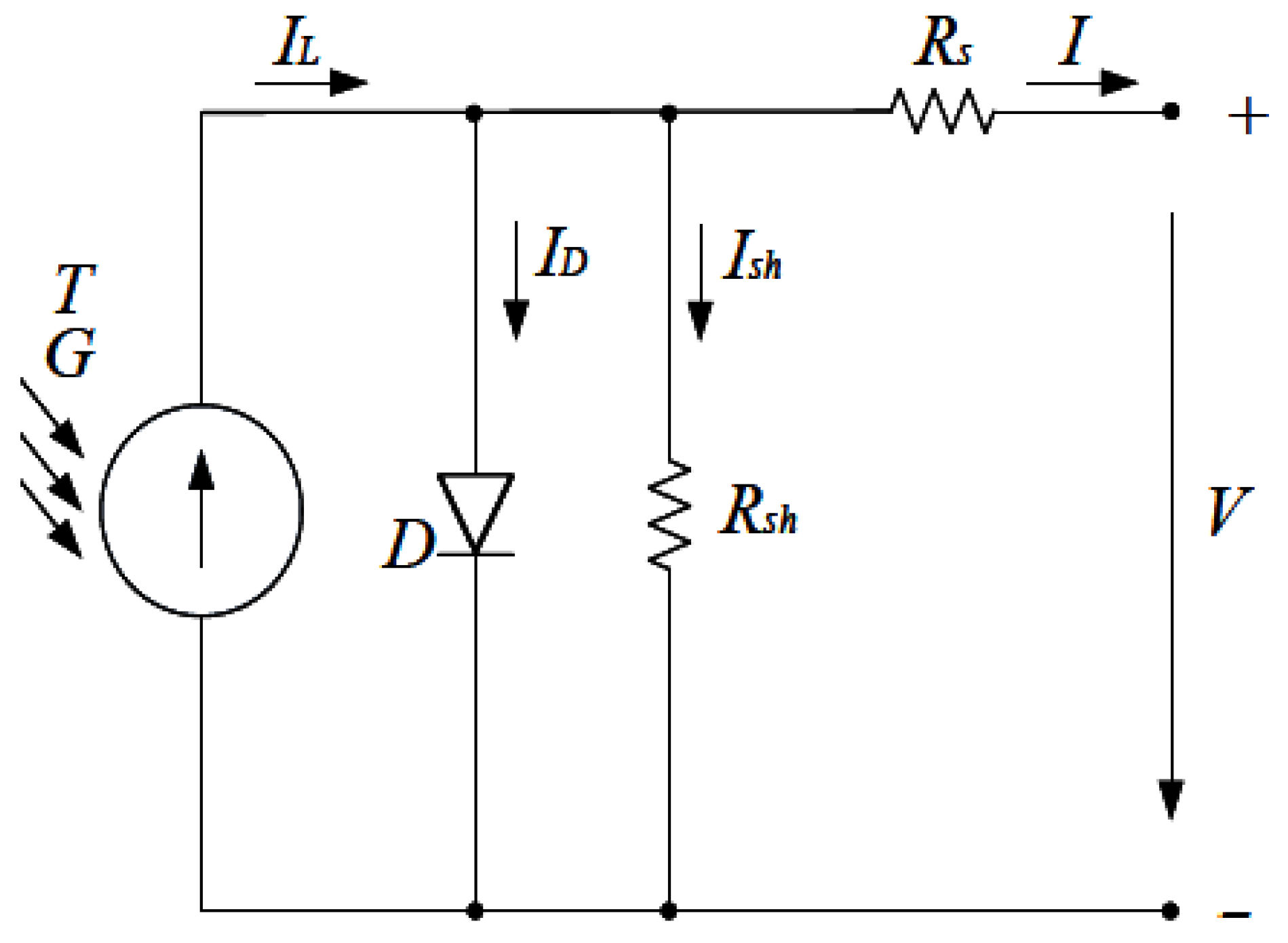
2.1. The Five-Parameter PV Cell Model

The five-parameter PV cell model is based on the circuit equivalent of Figure 1. It consists of a DC source generating the photocurrent I L , a p-n junction, representing the semiconductor response of the PV cell, and two internal ohmic resistances, one series and one shunt which represent operating losses. The output of the DC source depends on the irradiance G of the cell and the temperature T on the surface of the cell. Its output of the p-n junction is a function of the properties of the semiconductor material used, the temperature, and the voltage applied at the p-n junction, i.e., the loading of the cell. The output current I is the difference between the photocurrent I L , the current I D drawn by the diode and the ohmic losses represented by the shunt resistor R s h
I = I L I D I s h
The DC photocurrent I L depends on the irradiance G and the temperature T on the surface of the cell:
I L = G G S T C I S C + K I T T S T C
where G S T C and T S T C are the irradiance and temperature in STC, 1000 W/m2 and 25   ° C , respectively, and I S C represents the short-circuit current in A, measured at STC. K I is the short-circuit current coefficient in A / ° C . All parameters are specific to a given panel and supplied by the manufacturer.
The current drawn by the diode I D is given by:
I D = I s e x p q V + I R s n k T 1
I s = I 0 T T S T C 3 e x p q E G 1 T S T C 1 T n k
where I s represents the p-n junction’s saturation current in A, V represents the output voltage in V, n is the diode ideality factor which varies between 1 and 2 and T is the p-n junction temperature in K. I 0 is the reverse saturation current and E G is the band gap energy of the p-n junction. k = 1.3806 × 10 23 J/K is the Boltzmann constant and q = 1.602 × 10 19   ° C is the charge of the electron. V o c is the open circuit voltage in V, and R s h is the shunt resistance in Ω.
The shunt resistance current I s h is given by:
I s h = V + I R s R s h
It is worth noting that if the parallel resistance R s h is sufficiently greater than the load resistance that can be connected to the ends of the model and the series resistance R s is sufficiently less than the load resistance, then the losses just mentioned may be considered negligible.
The power output P , in W, of the PV cell is calculated as P = V I . The power output is zero at V = V o c where I = 0, and I = I s c where V = 0 . Consequently, there exists a specific pair of current and voltage values, I m p and V I m p , respectively, where the output power is maximized, P m a x = V m p I m p . This combination is known as the Maximum Power Point (MPP) and denotes the ideal operational point of a PV cell and is a crucial parameter for PV system design and performance optimization. Equations (1)–(5) describe the model used for the calculations shown below.

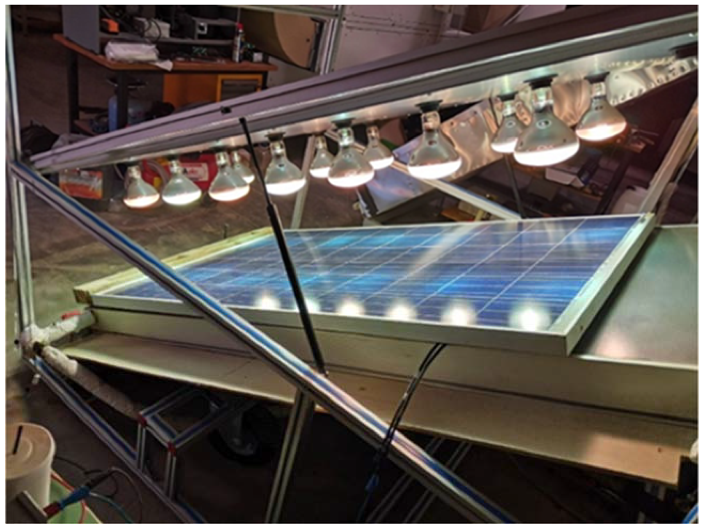
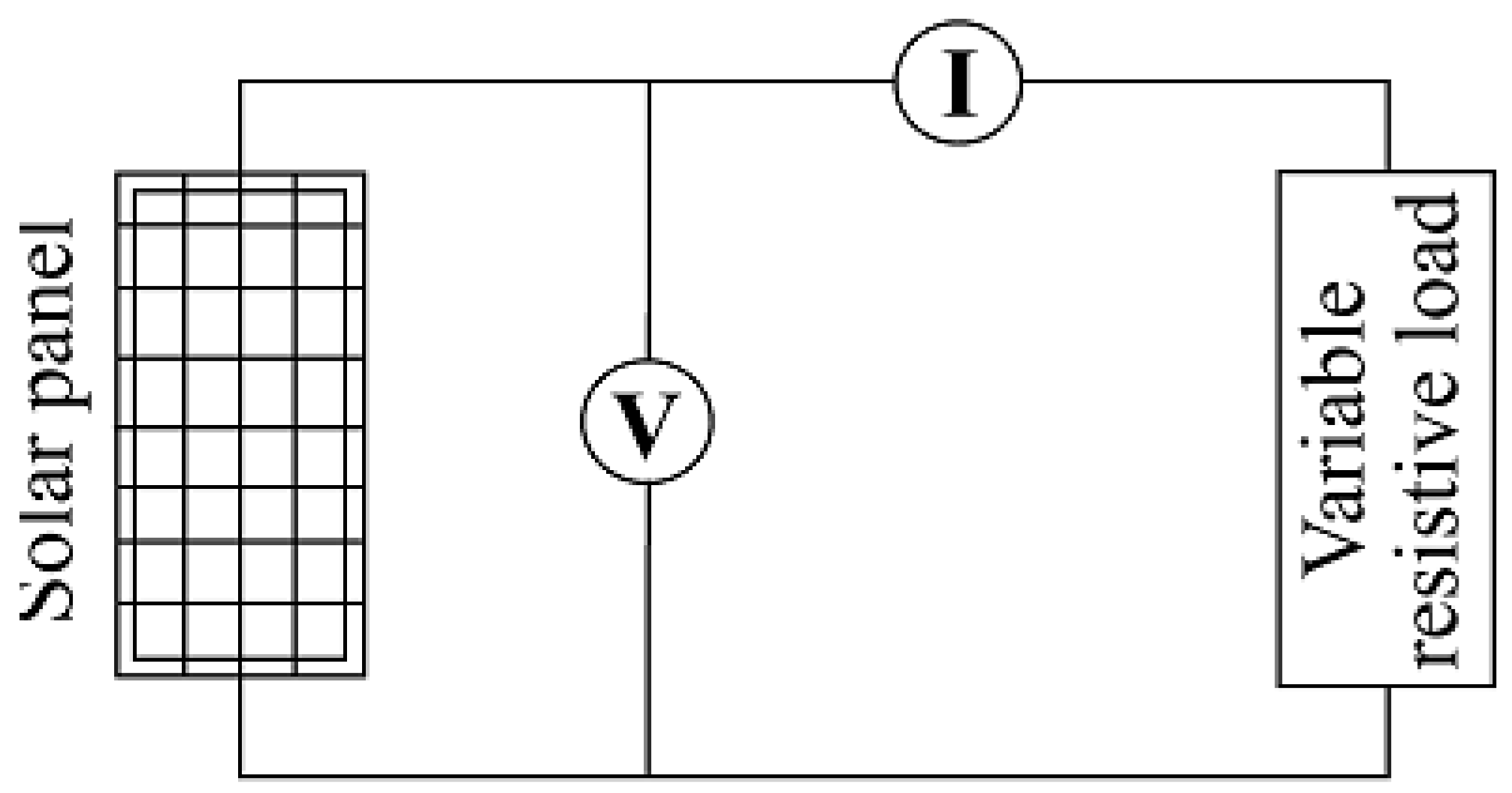
2.2. Lab Measurements of PV Module Outputs (Voltage, Current and Irradiation)

The experiment was conducted using the infrastructure of the Renewable Energy Sources Laboratory, NKUA—Euripus Complex which consists of a PV panel and an array of 14 lamps as shown in Figure 2. The inclination of the panel with respect to the lamp array may be controlled and is varied from 0.0 ° to 9.0 ° . The distance between the PV panels and the lamps at 0.0 ° inclination is 0.5 m. The specifications of the solar panel and lamps used are given in Table 1 and Table 2.
The lamps are arranged in a 7 × 2 matrix. The series of measurements are repeated for two arrangements: (1) All lamps are on (2) The lamps alternately lit, as shown in the diagrams below (Figure 3), to emulate shading.
A variable resistor was connected to the panel output to control the output voltage V, as shown in Figure 4. The voltage V and current I of the load were measured as shown by two multimeters with specifications as shown in Table 3. The voltage varied from 0 to 31.2 V with a step of 0.5 V.
The temperature on the surface of the panel was measured at the top-left and bottom-right corners using T-type thermocouples whose specifications are shown in Table 3.
The irradiance was measured for both lamp arrangements at the center of each cell for all 60 cells using an ISO9060:1990 [25]. First Class certified pyranometer combined with a data logger whose specifications are shown in Table 4 and Table 5, respectively. The I-V curves were obtained for the two lighting schemes as shown in Figure 3 and three inclinations φ = 0.0 ° , φ = 4.5 ° , φ = 9.0 ° . After every set of measurements, the temperature of the PV module surface was captured by a thermal camera whose specifications are shown (Table 6). The P-V curves were computed from the 6 I-V curves measured using the methodology described.

3. Results

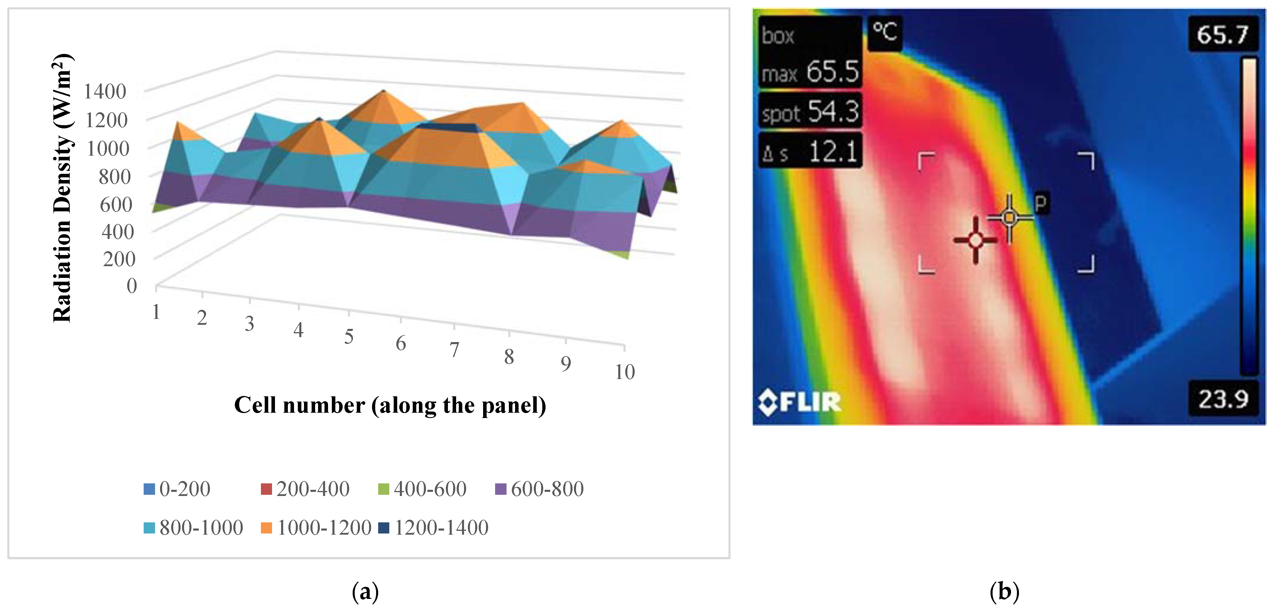
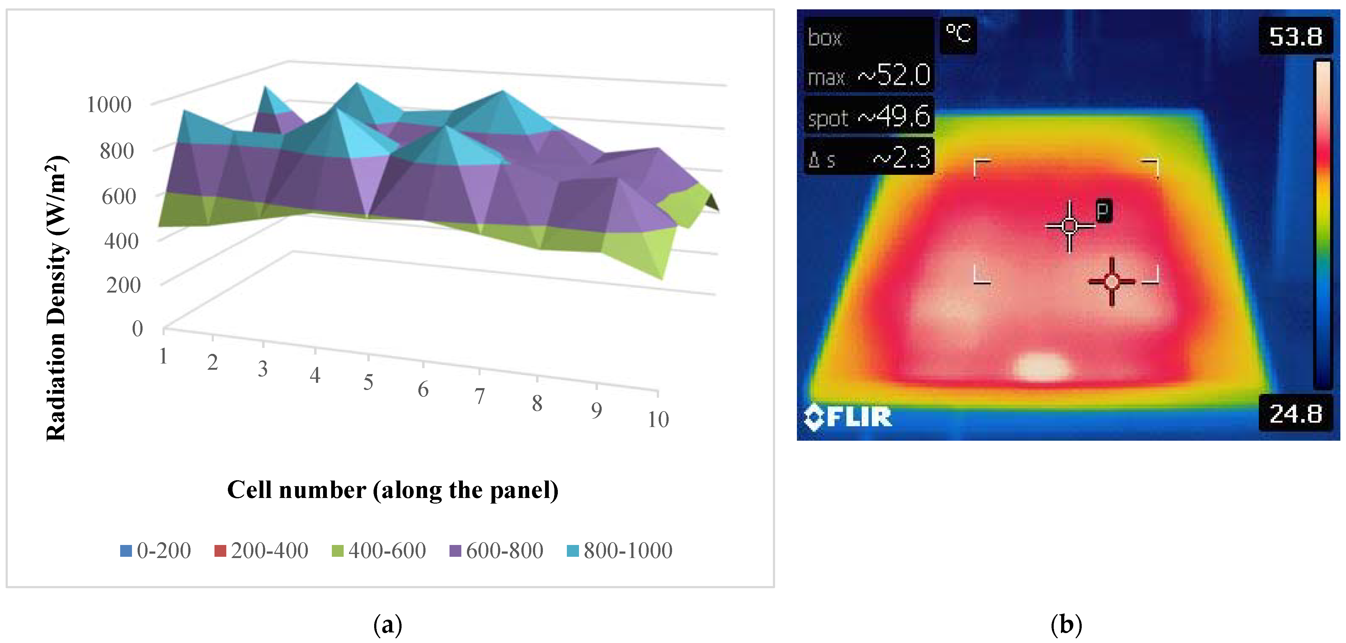
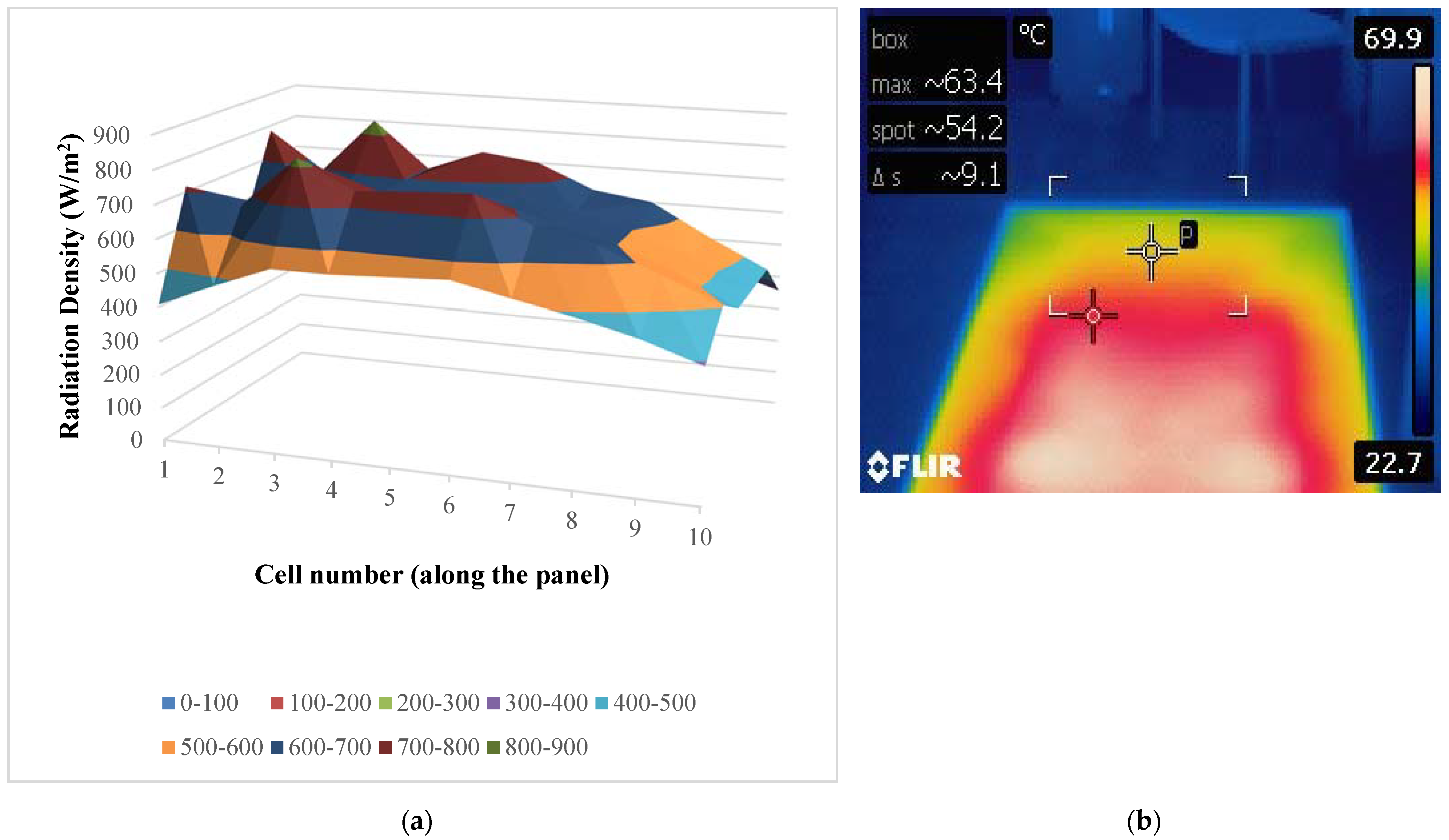
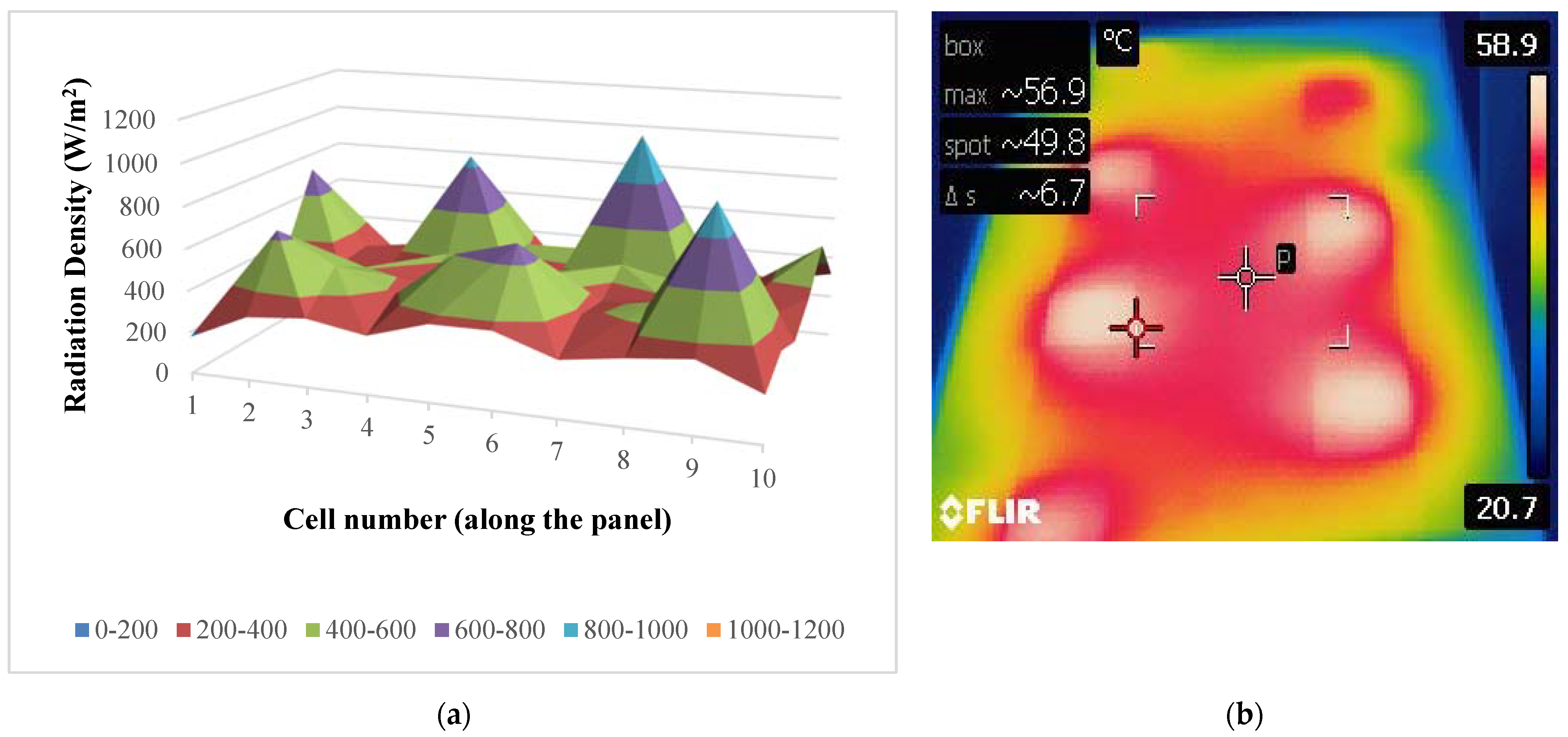
3.1. Temperature and Irradiance Distribution Measurements

For each inclination and lighting Arrangement, we display the results of the solar irradiation distribution on the panel’s surface as measured by the pyranometer and the temperature distribution as captured by the thermal camera.
We also provide the measurements used as input variables and parameters to the 5-parameter model. Namely:
-
temperature T as measured by the thermocouple
-
open voltage circuit, V o c
-
short-circuit current, I s c
-
the average irradiation, G a v e

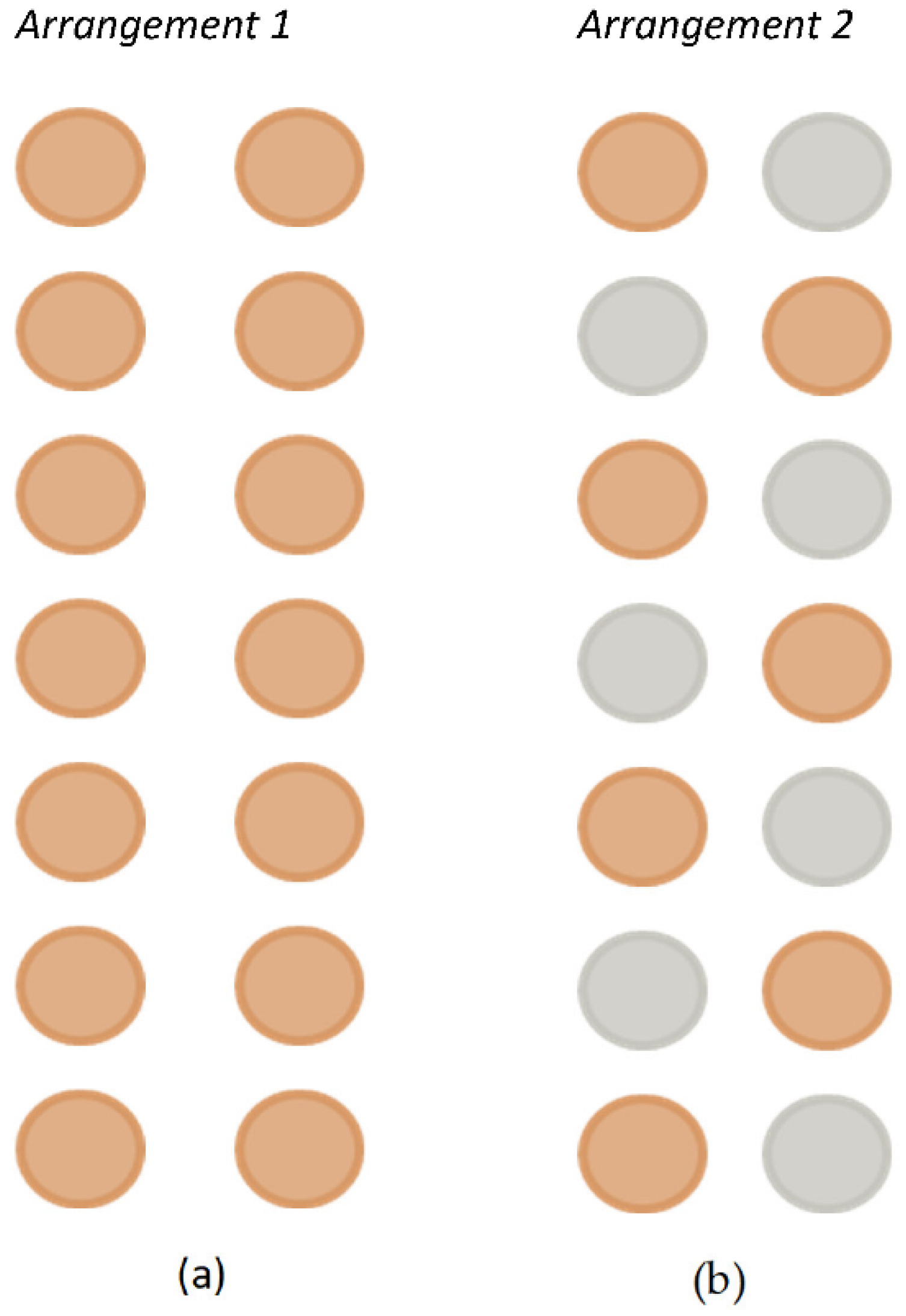
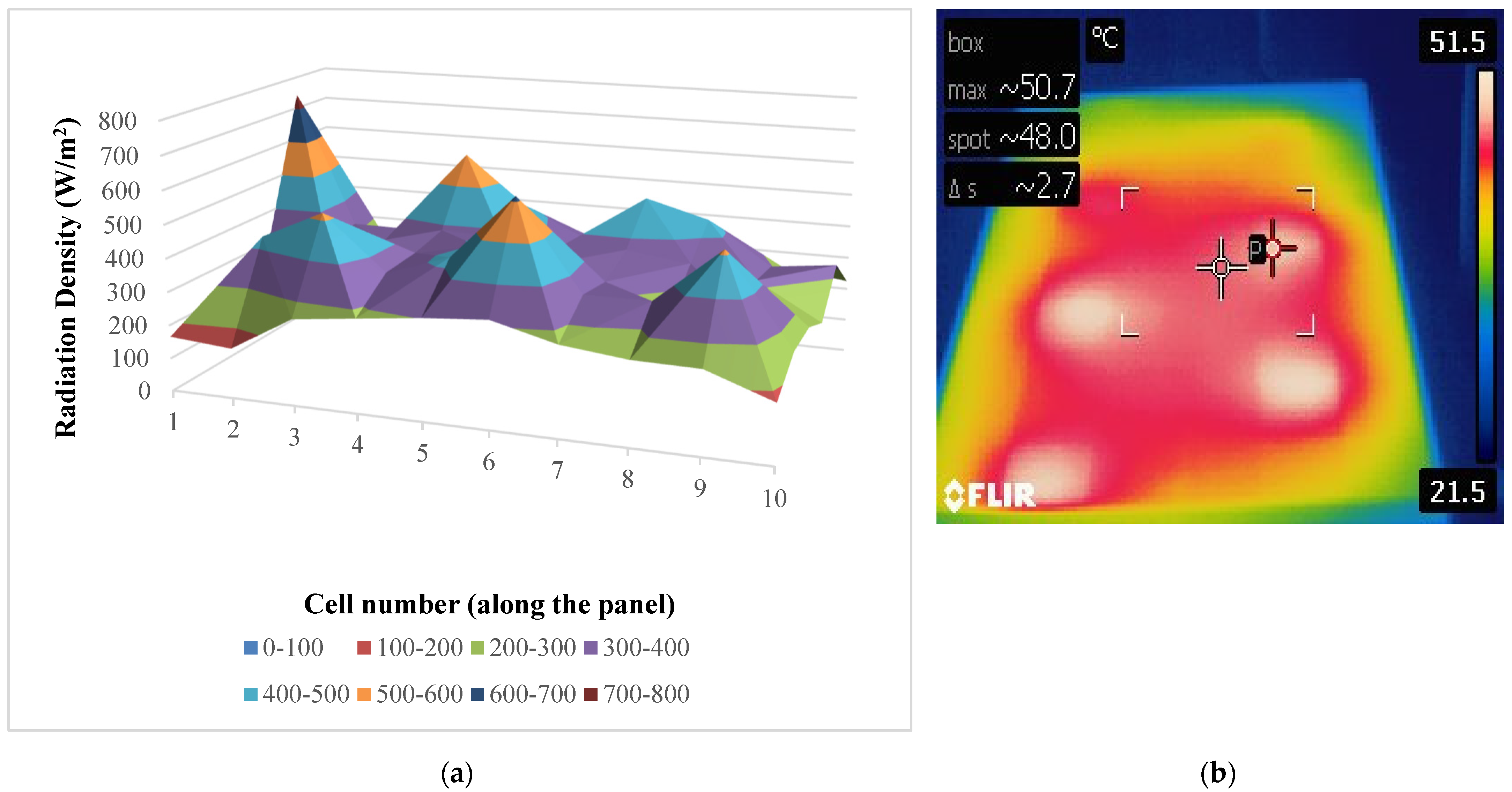
3.1.1. Arrangement 1: All Lamps Are Lit, Inclinations φ = 0.0 ° , 4.5 ° and 9.0 °

The irradiance on the surface of the panel in the inclination φ = 0.0 ° (Figure 5) ranges from 422 W/m2 at the top-right cell to 1223 W/m2 in one of the middle cells which is directly underneath the lamp. In this inclination, the PV panel receives the highest irradiation as it is parallel to the matrix of the lamps. The measurements used in the simulations of the next section are: V o c = 34.00   V , I s c = 3.40   A , T = 51.5   ° C , G a v e = 800.55   W / m 2 . The PV panel is positioned at an inclination φ = 4.5 ° (Figure 6) in which irradiance on the surface ranges from 450 W/m2 at the bottom-left cell to 986 W/m2 in one of the middle cells which are directly underneath a lamp. As can be easily understood in this scenario, the irradiance is lower than φ = 0.0 ° and higher than the angle of 9.0 ° . The measurements used in the simulations of the next section are: V o c = 33.50   V , I s c = 1.83   A , T = 45   ° C , G a v e = 681.05   W / m 2 . Lastly, the irradiance incident in the panel for the inclination φ = 9.0 ° (Figure 7) ranges from 390 W/m2 in the bottom-left cell to 837 W/m2 in one of the top-right cells. The measurements used in simulations are: V o c = 28.80   V , I s c = 1.60   A , T = 43   ° C , G a v e = 593.70   W / m 2 .

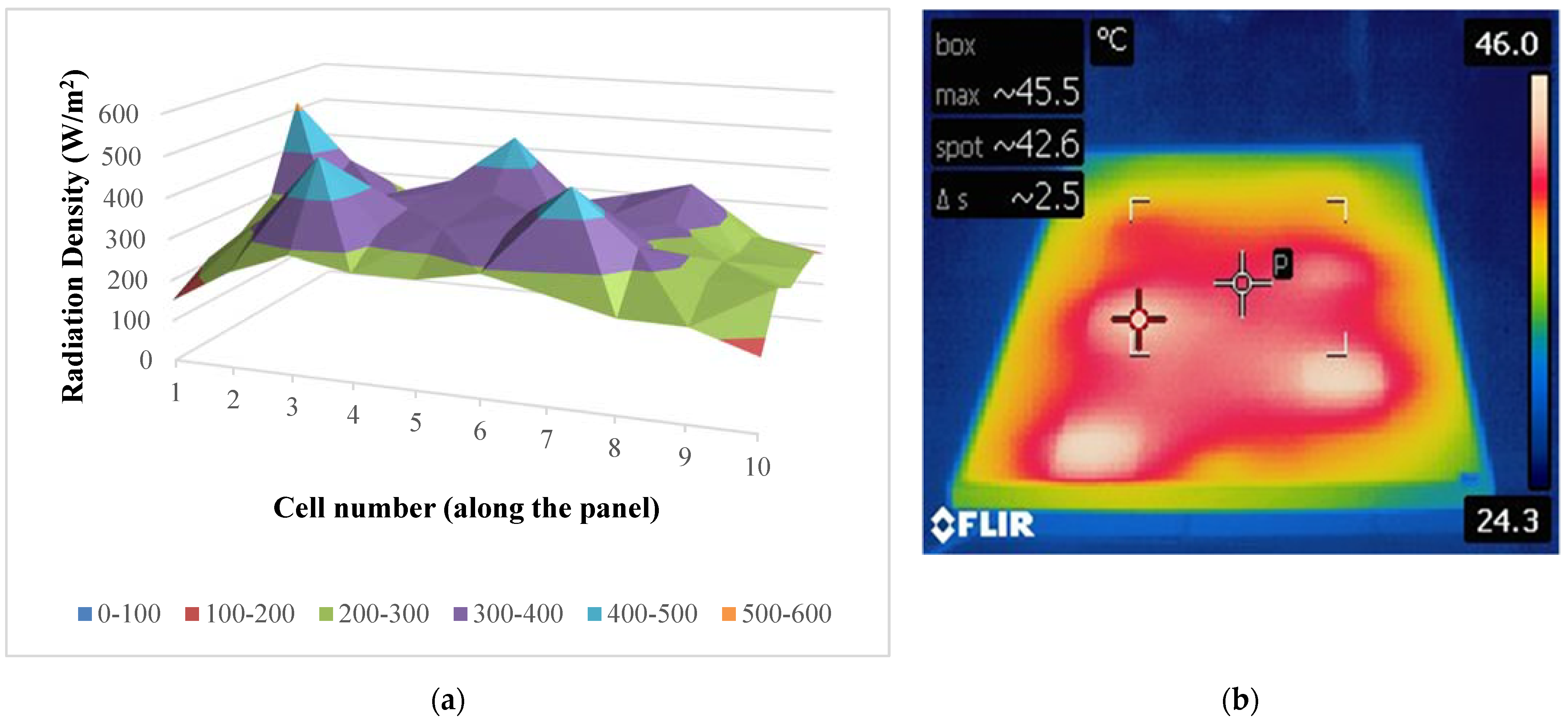
3.1.2. Arrangement 2: Lamps Alternately Lit, Inclinations φ = 0.0 ° , 4.5 ° and 9.0 °

The second arrangement was used to study the effect of more intense variations of the irradiance distribution. The irradiance incident in the panel for the inclination φ = 0.0 ° , (Figure 8) ranges from 177 W/m2 in the upper-left corner cell to 946 W/m2 in one of the bottom-left cells. The measurements used in the simulations of the next section are: V o c = 32.00   V , I s c = 2.00   A , T = 43   ° C , G a v e = 398.97   W / m 2 . For the inclination φ= 4.5 ° (Figure 9) irradiance on the surface of the PV module ranges from 165 W/m2 in the same cell as the previous case to 742 W/m2 in one of the upper-right cells. The measurements used in the simulations of the next section are: V o c = 29.50   V , I s c = 0.94   A , T = 41   ° C , G a v e = 334.67   W / m 2 . In the third scenario in which the biggest inclination φ = 9.0 ° (Figure 10), the irradiance on the surface ranges from 150 W/m2 in the upper-left cell to 519 W/m2 in one of the upper-right cells. The measurements used in the simulations of the next section are: V o c = 29.10   V , I s c = 0.89   A , T = 39.5   ° C , G a v e = 293.52   W / m 2 .

3.1.3. Summary Table of Measurements for All Cases

In Table 7, we summarize the measured values, V o c , I s c , T, G a v e , for each case which will be used in the following simulations. We also include the maximum, minimum, and standard deviation of the irradiance values, G m a x , G m i n and G s d , respectively.

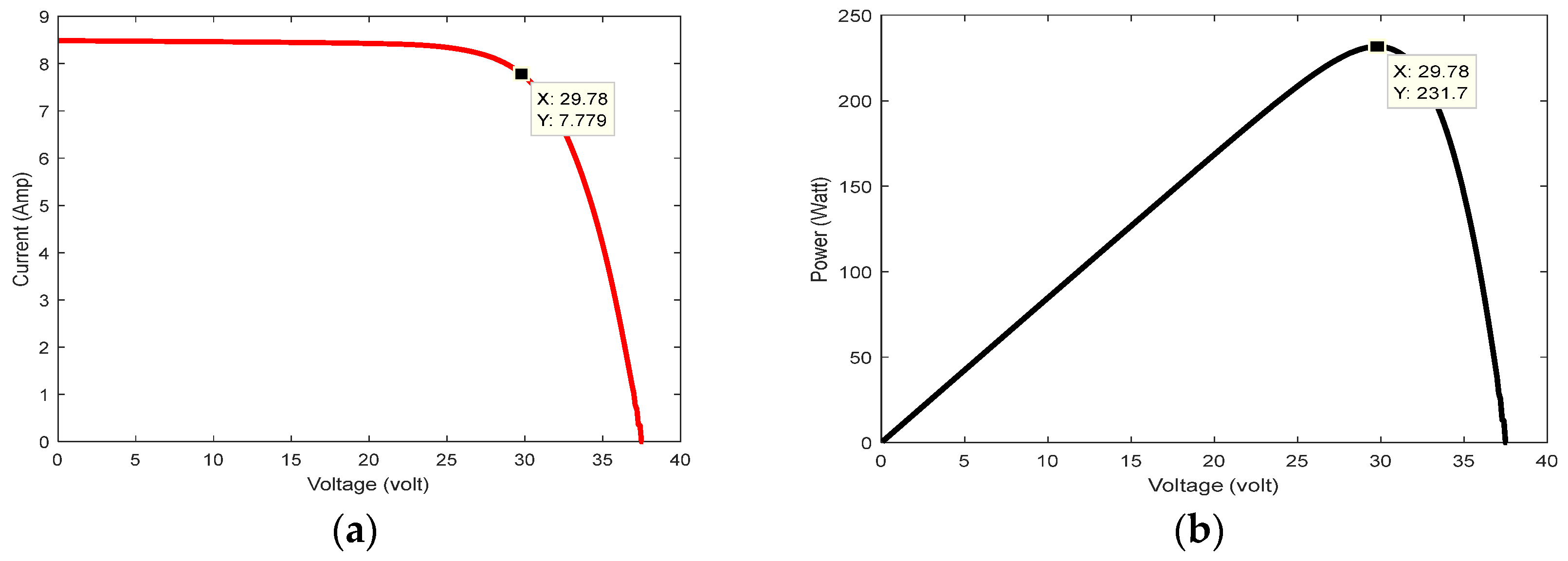
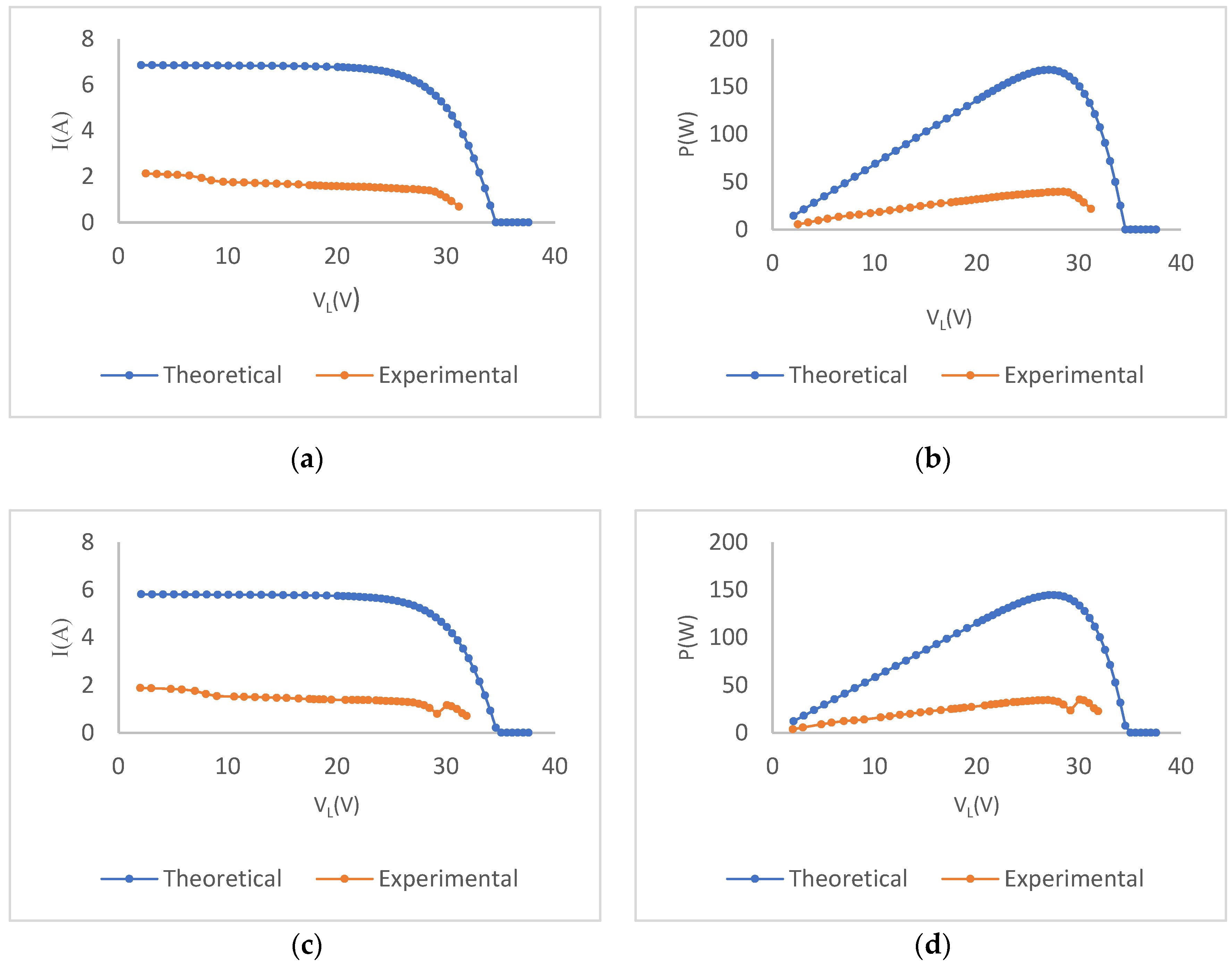
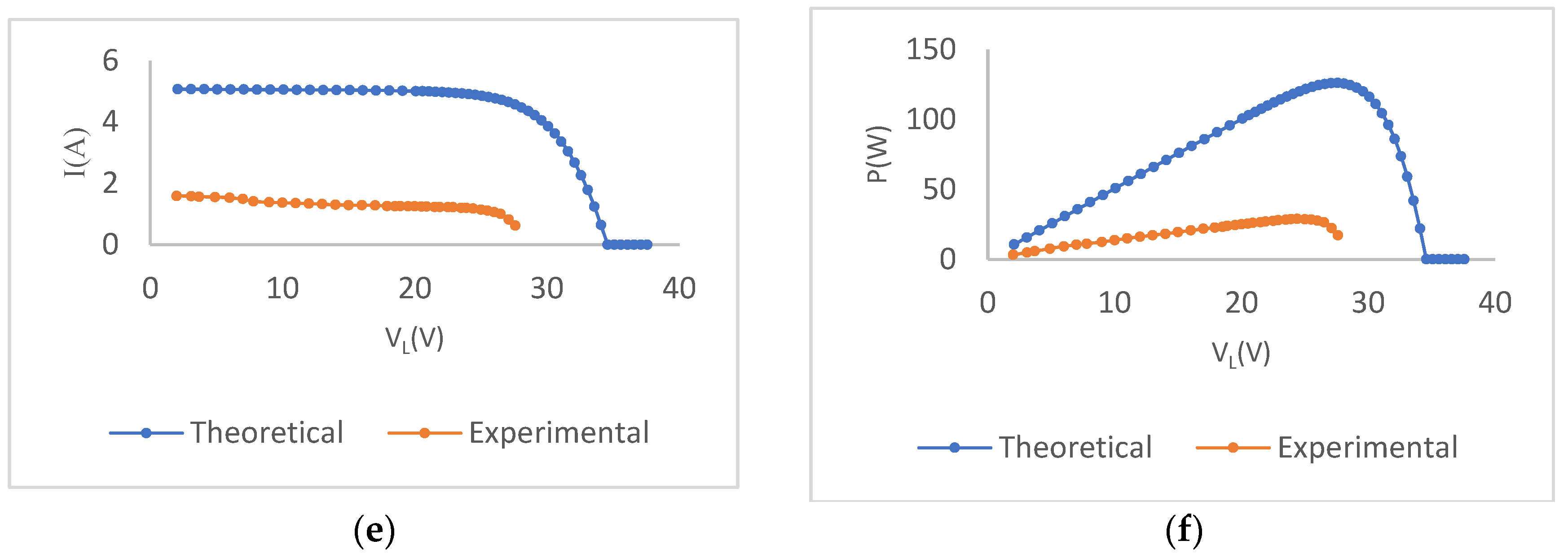
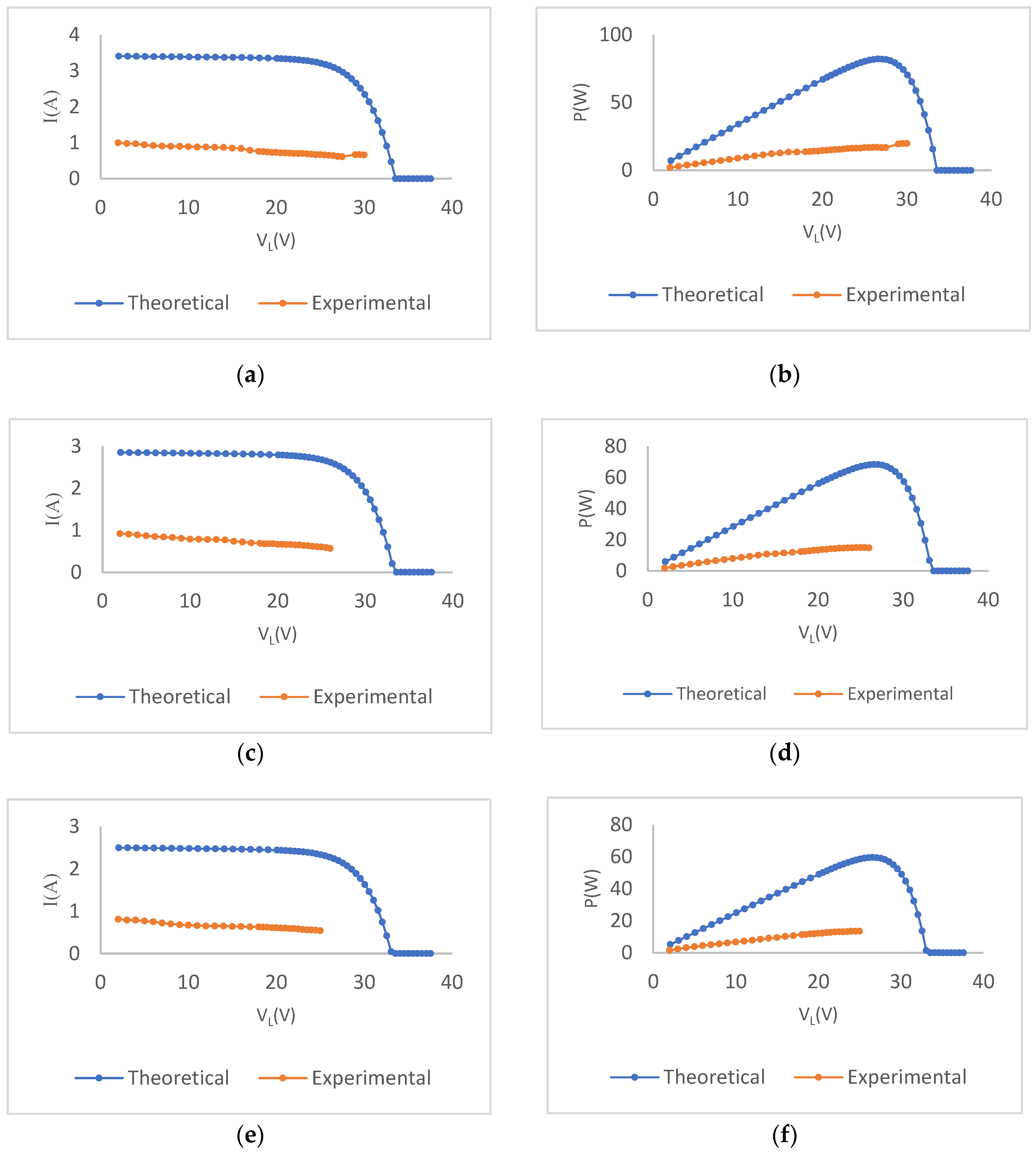
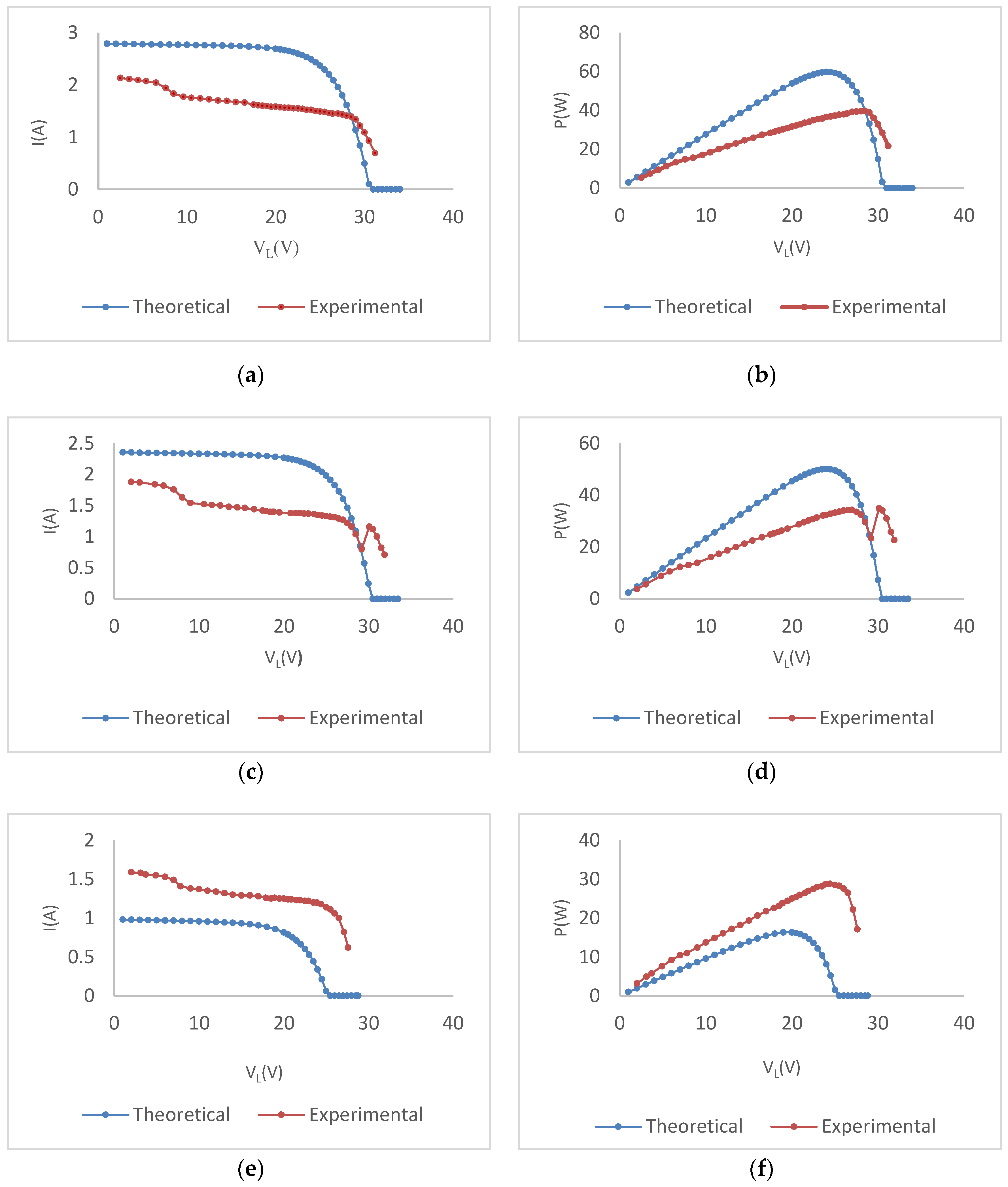
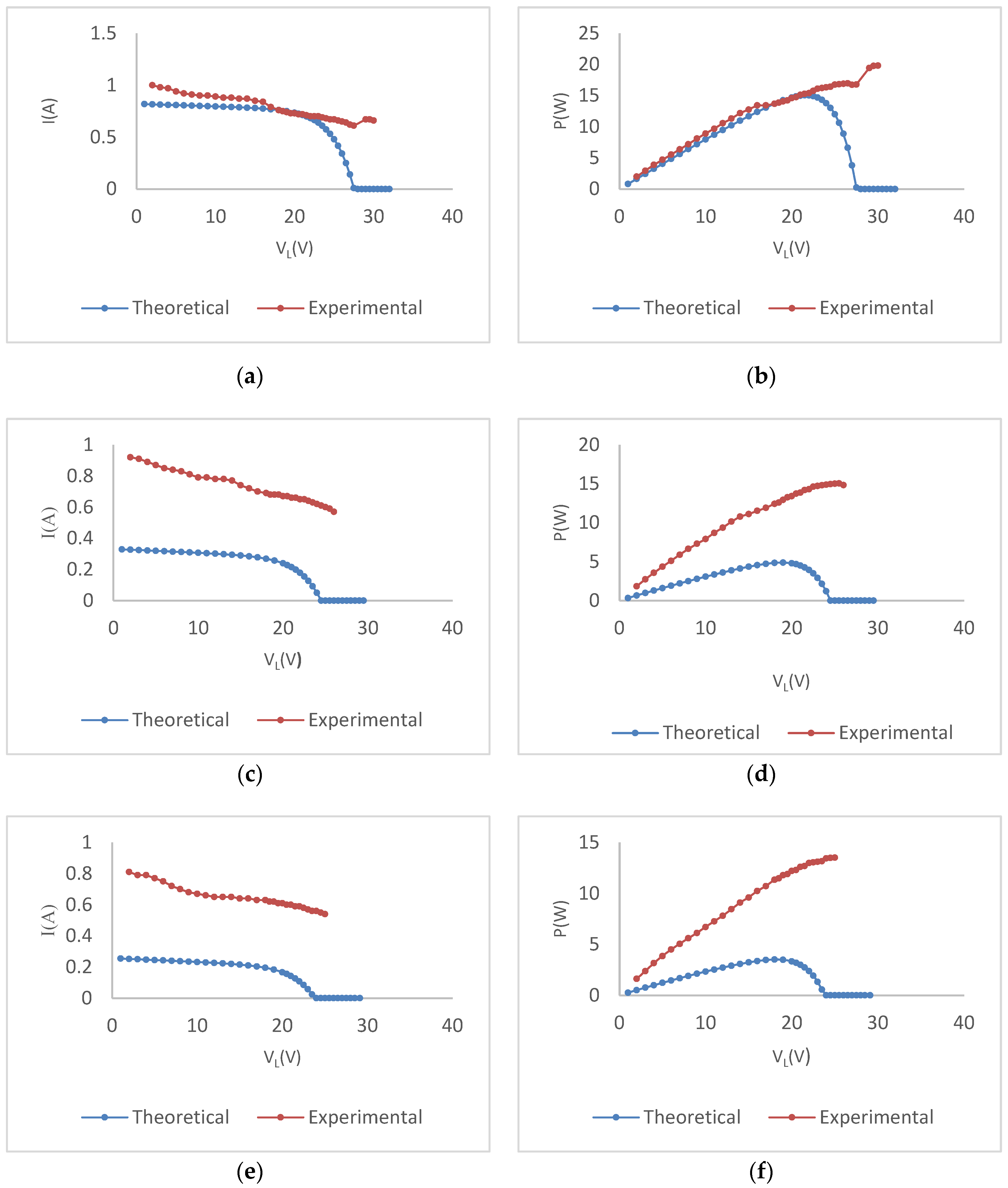
3.2. Modeling and Simulation Results

The five-parameter model given in Equations (1)–(5) was implemented on GNU Octave and identified for the STC parameters (Figure 11) of the manufacturer’s specifications (Table 1). The values obtained for the two resistors were R s h = 415.00   Ω and R s = 0.22   Ω . Next, two sets of simulated curves are presented and compared to the measured ones, for each one of the six cases. Figure 12 and Figure 13 display the measured I-V and P-V curves compared against the simulated curves for all inclinations and arrangements. The G and T values used are the measured ones. The V o c and I s c are the values provided by the manufacturer.
Given the discrepancy observed between the measured and calculated curves, we repeated the simulations (Figure 14 and Figure 15) using the average measured G and T values, as before, while the measured V o c and I s c were used instead, as shown in Table 7 for each case. The simulated curves show smaller deviations than the experimental ones.

4. Discussion

The experimental results provided insights into the effect of the distribution of irradiance and temperature values on a panel. The simulated results showed the limitations of the five-parameter model when the irradiance and temperature on the surface are not uniform, or the model parameters deviate from those measured at STC.
As expected, the use of the 7 × 2 lamp matrix leads to higher solar radiation areal density underneath the lamps compared to the cells that are not directly underneath a lamp. Similarly, the temperature distribution is highly non-uniform, as shown by the thermal camera pictures. The irradiance varies from 1223.00 W/m2 when all lamps are lit (Arrangement 1) and the inclination is 0.0 ° , to 150.00 W/m2 when half of the lamps are lit (Arrangement 2) and the inclination is 9.0 ° . The temperature is highest at the center of the panel and especially under the lamps, reaching 70   ° C , and decreases towards the edges where it was measured as low as 20   ° C .
Varying the inclination of the panel leads to smaller differences between maximum and minimum irradiance values which is reflected in the standard deviation of the measured values as well as the temperature dependence measured by the thermocouples (see Table 7).
Arrangement 2, where half of the lamps are lit, results in irradiance values that are 50% lower than those of Arrangement 1, where all lamps are on, for all inclinations. A similar trend is observed in the measured values of I s c which demonstrates the strong dependence of the DC output on irradiance.
Overall, reduced irradiance and an increase in temperature both result in power reduction. The I-V and P-V curves obtained experimentally also show the effect of the non-uniform irradiance and related spotted heating. The fact that the regions under higher irradiance are also those with higher temperatures limits the gains for the higher irradiance levels. This is most evident in the cases of inclination 0.0 ° and 4.5 ° for Arrangement 1 (Figure 14a–d). When φ = 0.0 ° , the highest G levels are measured, but also the highest temperatures are recorded, and the power output is comparable to the case of φ = 4.5 ° .
The simulation results (Figure 12, Figure 13, Figure 14 and Figure 15) have a higher discrepancy with the measured ones when the STC values for I s c and V o c are used in the model which is reasonable. The simulated curves demonstrate approximately three times higher output current values for a given output voltage value, for all inclinations and both arrangements.
However, when the measured I s c and V o c (Table 7) are used instead, the discrepancy decreases and the computed values of the output current are underestimated with two exceptions: in the case of Arrangement 1, φ = 9.0 ° , the computed values of the output current are higher than the measured ones while in the case of Arrangement 2, φ = 0.0 ° , the agreement between measurement and calculations is good.
These discrepancies are due to the highly non-uniform irradiance and temperature distribution on the surface of the panel. The average value of the measured radiation is not a good approximation for the active radiation received by the panel in any case, leading sometimes to an overestimation and sometimes to an underestimation of the value. When specific cells receive higher irradiance levels, they tend to generate more electrical current. However, due to the simultaneous increase in temperature associated with the higher irradiance, the efficiency of these cells may diminish, resulting in a complex trade-off between irradiance and temperature effects. The temperature rise potentially results in a smaller gain in power output than what would be anticipated based solely on irradiance levels. In addition, voltage and current measurements are made at the load, while the model calculates the generated power of the PV panel without taking into account any losses in the circuit. The sensitivity of the PV panel performance on temperature and the limitation of the 5-parameter model to fully capture this effect is also discussed in [18]. The effect of increased losses due to the shunt resistance, as temperature increases will be studied in our future work.
Ongoing work focuses on carrying out the modeling for each cell separately using the measured G and T values for each cell and reconstructing the I-V curve for the whole panel. A similar approach has been used in [26] to model the effect of partial shading using two I-V curves. In our case, we will combine 60 I-V curves, one for each cell.
Another observation is that the measured output current curves exhibit a decreasing trend with increasing voltage which deviates from the diode model. This may be due to the measurement methodology since the measurements are taken continuously at successive loads and reaching higher voltage values requires more time and hence the temperature increases. However, this point needs to be further investigated.
Comparing the results shown here with those in the literature is not straightforward as they all focus on measurements carried out under actual solar irradiance and not artificial lighting. However, there seem to be several approaches to effectively using the 5-parameter model to reproduce measurements on PV panels when the operation conditions vary significantly from STC. A method for parameter extraction is proposed in [22] with the limitation that it applies to a PV panel with small output. This approach will be used in future work to better understand the effect of spotted heating on the PV panel performance, and its modelling [27,28,29,30,31,32,33,34,35,36,37,38,39,40,41,42,43,44,45,46,47,48,49,50,51,52,53,54,55,56].

5. Conclusions

In this paper, an experiment using artificial lighting of a PV panel was designed to study the effect of highly non-uniform irradiance and temperature distribution on the surface of a PV panel. Artificial lighting was used to generate various irradiance and temperature profiles and the DC output was measured at various loading conditions to obtain the corresponding I-V and P-V curves. The irradiance was recorded at each cell of the PV panel while the temperature distribution was measured using a thermal camera. The overall temperature was measured using a pair of thermocouples. The spotted lighting resulted in the cells with the highest irradiance also having the highest temperature which considerably limited the gains for the high irradiance.
Next, the 5-parameter model was used to study its performance for such non-uniform temperature and irradiance profiles. The results showed that there is a significant deviation between the experimental and simulated results since the simulation does not account for the non-uniformity of the irradiance and temperature profiles. Again, the temperature seems to play a significant role in determining the DC output. This role seems to not be fully captured by the model.
The experimental findings underscored the importance of acknowledging the non-uniform distribution of irradiance (solar energy input) and temperature across the PV panel’s surface. Real-world conditions often involve variations in shading, obstructions, and local temperature differences that can lead to differing levels of irradiance and temperature exposure on various parts of the panel. This non-uniformity impacts the overall panel performance by creating gradients in electrical characteristics and efficiency across its surface. The 5-parameter model seems to be insufficient for variable temperatures and irradiance values. This experiment could act as a starting point for future model improvement regarding irradiance and temperature variables, for more effective design and implementation against weather conditions, and for testing PV panels in different than STC conditions.
This result leads our efforts towards obtaining a calculated I-V characteristic for each cell and then combining them to reconstruct the I-V curve of the whole panel. This is a tedious process, but we expect that it will account for the effect of the non-uniformity in the temperature and irradiance distribution. Based on these results, modifications to the existing model will be proposed to develop an efficient modeling tool for cases where non-uniform lighting is expected.

Author Contributions

Conceptualization, A.K.; methodology, A.K. and J.K.; software, P.T. and J.K.; validation, P.T., J.K. and P.K.; formal analysis, P.T. and P.K.; investigation, P.T. and M.V.; resources, M.V.; data curation, P.T., P.K. and A.K.; writing—original draft preparation, P.T. and P.K.; writing—review and editing, A.K.; visualization, P.T., J.K. and P.K.; supervision, A.K.; project administration, A.K. and M.V. All authors have read and agreed to the published version of the manuscript.

Funding

This research received no external funding.

Data Availability Statement

All data used and produced for this study can be requested from the corresponding author.

Acknowledgments

The authors would like to acknowledge the support of the Renewable Sources Laboratory for providing materials and technical staff to carry out this research. P.K. acknowledges the EU-funded CiROCCO project under Grant Agreement No 101086497 and the ClimSA Programme which is an initiative funded by the European Union and implemented by the Organisation of African, Caribbean, and Pacific States (OACPS).

Conflicts of Interest

The authors declare no conflict of interest.

References

  1. Anjos, R.S.; Melicio, R.; Mendes, V.M.F.; Miguel, H. Crystalline Silicon PV Module under Effect of Shading Simulation of the Hot-Spot Condition. In Proceedings of the Technological Innovation for Smart Systems: 8th IFIP WG 5.5/SOCOLNET Advanced Doctoral Conference on Computing, Electrical and Industrial Systems, DoCEIS 2017, Costa de Caparica, Portugal, 3–5 May 2017; pp. 479–487. [Google Scholar] [CrossRef]
  2. Kabir, E.; Kumar, P.; Kumar, S.; Adelodun, A.A.; Kim, K.-H. Solar energy: Potential and future prospects. Renew. Sustain. Energy Rev. 2018, 82, 894–900. [Google Scholar] [CrossRef]
  3. Milosavljević, D.D.; Pavlović, T.M.; Piršl, D.S. Performance Analysis of a Grid-Connected Solar PV Plant in Niš, Republic of Serbia. Renew. Sustain. Energy Rev. 2015, 44, 423–435. [Google Scholar] [CrossRef]
  4. Lo Brano, V.; Orioli, A.; Ciulla, G.; Di Gangi, A. An Improved Five-Parameter Model for Photovoltaic Modules. Sol. Energy Mater. Sol. Cells 2010, 94, 1358–1370. [Google Scholar] [CrossRef]
  5. Chikate, B.V.; Sadawarte, Y.A. The Factors Affecting the Performance of Solar Cell. Int. J. Comput. Appl. 2015, 1, 0975–8887. [Google Scholar]
  6. Fialho, L.; Melício, R.; Mendes, V.; Viana, S.; Rodrigues, C.; Estanqueiro, A. A simulation of integrated photovoltaic conversion into electric grid. Sol. Energy 2014, 110, 578–594. [Google Scholar] [CrossRef]
  7. Sarkar, M.N.I. Effect of Various Model Parameters on Solar Photovoltaic Cell Simulation: A SPICE Analysis. Renew. Wind. Water Sol. 2016, 3, 13. [Google Scholar] [CrossRef]
  8. Abbassi, R.; Abbassi, A.; Jemli, M.; Chebbi, S. Identification of Unknown Parameters of Solar Cell Models: A Comprehensive Overview of Available Approaches. Renew. Sustain. Energy Rev. 2018, 90, 453–474. [Google Scholar] [CrossRef]
  9. Ramadan, A.; Kamel, S.; Taha, I.B.M.; Tostado-Véliz, M. Parameter Estimation of Modified Double-Diode and Triple-Diode Photovoltaic Models Based on Wild Horse Optimizer. Electronics 2021, 10, 2308. [Google Scholar] [CrossRef]
  10. Patel, M.R. Wind and Solar Power Systems; CRC Press: Boca Raton, FL, USA, 1999. [Google Scholar]
  11. Vidyanandan, K.V. An Overview of Factors Affecting the Performance of Solar PV Systems. Energy Scan 2017, 27, 216. [Google Scholar]
  12. Mansouri, N.; Lashab, A.; Sera, D.; Guerrero, J.M.; Cherif, A. Large Photovoltaic Power Plants Integration: A Review of Challenges and Solutions. Energies 2019, 12, 3798. [Google Scholar] [CrossRef]
  13. Roumpakias, E. Development of Methodologies for Performance Analysis of Grid-Connected Photovoltaic Systems. Available online: https://www.didaktorika.gr/eadd/handle/10442/46825 (accessed on 16 February 2023).
  14. Rompotis, S.; Konstantaras, J.; Ktena, A.; Sarakis, L.; Manasis, C. A Monitoring System for PV plants using Open Technologies. In Proceedings of the 2022 IEEE 7th International Energy Conference (ENERGYCON), Riga, Latvia, 9–12 May 2022; pp. 1–5. [Google Scholar]
  15. Lineykin, S.; Averbukh, M.; Kuperman, A. Five-Parameter Model of Photovoltaic Cell Based on STC Data and Dimensionless. In Proceedings of the 2012 IEEE 27th Convention of Electrical and Electronics Engineers in Israel, Eilat, Israel, 14–17 November 2012. [Google Scholar] [CrossRef]
  16. Prakash, R.; Singh, S. Designing and Modelling of Solar Photovoltaic Cell and Array. IOSR J. Electr. Electron. Eng. (IOSR-JEEE) 2016, 11, 35–40. [Google Scholar] [CrossRef]
  17. Hamou, S.; Zine, S.; Abdellah, R. Efficiency of PV Module under Real Working Conditions. Energy Procedia 2014, 50, 553–558. [Google Scholar] [CrossRef]
  18. Celik, A.N.; Acikgoz, N. Modelling and Experimental Verification of the Operating Current of Mono-Crystalline Photovoltaic Modules Using Four- and Five-Parameter Models. Appl. Energy 2007, 84, 1–15. [Google Scholar] [CrossRef]
  19. Fialho, L.; Melício, R.; Mendes, V.M.; Figueiredo, J.; Collares-Pereira, M. Amorphous Solar Modules Simulation and Experimental Results: Effect of Shading. In Proceedings of the 5th Doctoral Conference on Computing, Electrical and Industrial Systems (DoCEIS), Costa de Caparica, Portugal, 7–9 April 2014; pp. 315–323. Available online: https://inria.hal.science/hal-01274793/ (accessed on 16 February 2023).
  20. Dondi, D.; Brunelli, D.; Benini, L.; Pavan, P.; Bertacchini, A.; Larcher, L. Photovoltaic Cell Modeling for Solar Energy Powered Sensor Networks. In Proceedings of the 2007 2nd International Workshop on Advances in Sensors and Interface, Bari, Italy, 26–27 June 2007. [Google Scholar] [CrossRef]
  21. Goss, B.; Cole, I.; Betts, T.; Gottschalg, R. Irradiance Modelling for Individual Cells of Shaded Solar Photovoltaic Arrays. Sol. Energy 2014, 110, 410–419. [Google Scholar] [CrossRef]
  22. Subudhi, B.; Pradhan, R. Characteristics Evaluation and Parameter Extraction of a Solar Array Based on Experimental Analysis. In Proceedings of the 2011 IEEE Ninth International Conference on Power Electronics and Drive Systems, Singapore, 5–8 December 2011. [Google Scholar] [CrossRef]
  23. Humada, A.M.; Darweesh, S.Y.; Mohammed, K.G.; Kamil, M.; Mohammed, S.F.; Kasim, N.K.; Tahseen, T.A.; Awad, O.I.; Mekhilef, S. Modeling of PV System and Parameter Extraction Based on Experimental Data: Review and Investigation. Sol. Energy 2020, 199, 742–760. [Google Scholar] [CrossRef]
  24. Salmi, T.; Bouzguenda, M.; Gastli, A.; Masmoudi, A. MATLAB/Simulink Based Modelling of Solar Photovoltaic Cell. Int. J. Renew. Energy Res. 2012, 2, 213–218. [Google Scholar]
  25. ISO9060:1990. Available online: https://www.iso.org/obp/ui/#iso:std:iso:9060:ed-1:v1:en (accessed on 16 February 2023).
  26. Xenophontos, A.; Bazzi, A.M. Model-Based Maximum Power Curves of Solar Photovoltaic Panels under Partial Shading Conditions. IEEE J. Photovolt. 2018, 8, 233–238. [Google Scholar] [CrossRef]
  27. Chenni, R.; Makhlouf, M.; Kerbache, T.; Bouzid, A. A Detailed Modeling Method for Photovoltaic Cells. Energy 2007, 32, 1724–1730. [Google Scholar] [CrossRef]
  28. Dolara, A.; Leva, S.; Manzolini, G. Comparison of Different Physical Models for PV Power Output Prediction. Sol. Energy 2015, 119, 83–99. [Google Scholar] [CrossRef]
  29. De Soto, W.; Klein, S.A.; Beckman, W.A. Improvement and Validation of a Model for Photovoltaic Array Performance. Sol. Energy 2006, 80, 78–88. [Google Scholar] [CrossRef]
  30. Stornelli, V.; Muttillo, M.; De Rubeis, T.; Nardi, I. A New Simplified Five-Parameter Estimation Method for Single-Diode Model of Photovoltaic Panels. Energies 2019, 12, 4271. [Google Scholar] [CrossRef]
  31. Ahmed, M.T. Modelization and Characterization of Photovoltaic-Panels. Master’s Thesis, University of Évora, Evora, Portugal, January 2017. [Google Scholar]
  32. Ahmed, T.; Gonçalves, T.; Albino, A.; Rashel, M.R.; Veiga, A.; Tlemçani, M. Different parameters variation analysis of a PV cell, In Proceedings of the International Conference for Students on Applied Engineering, Newcastle, UK, 20–21 October 2016.
  33. Alam, N.; Coors, V.; Zlatanova, S.; Oosterom, P.J.M. Shadow effect on photovoltaic potentiality analysis using 3d city models. In Proceedings of the International Archives of the Photogrammetry, Remote Sensing and Spatial Information Sciences, Melbourne, Australia, 25 August–1 September 2012; Volume XXXIX-B8. [Google Scholar]
  34. Bonkoungou, D.; Koalaga, Z.; Njomo, D. Modelling and simulation of photovoltaic module considering single diode equivalent circuit model in MATLAB. Int. J. Emerg. Technol. Adv. Eng. 2013, 3, 493–502. [Google Scholar]
  35. Paris Climate Change Conference, (FCCC/CP/2015/L.9/Rev.1), The Global Standard of Globalization is Not Limited to the Limitations of the System, XXI 2 °C. 2015. Available online: https://unfccc.int/resource/docs/2015/cop21/eng/l09r01.pdf (accessed on 29 August 2023).
  36. Demirel, Y. Energy: Production, Conversion, Storage, Conservation and Coupling; Springer, Springer International Publisher: Berlin/Heidelberg, Germany, 2016. [Google Scholar]
  37. Darwish, Z.A.; Kazem, H.A.; Sopian, K.; Alghoul, M.A.; Chaichan, M.T. Impact of some environmental variables with dust on solar photovoltaic (PV) performance: Review and research status. Int. J. Energy Environ. 2013, 7, 152–159. [Google Scholar]
  38. Elzinga, D. Electricity System Development: A Focus on—Smart Grids Overview of Activities and Players in Smart Grids; United Nations Economic Commission for Europe: Geneva, Switzerland, 2015. [Google Scholar]
  39. Foles, A.C.N. MPPT Study from a Solar Photovoltaic Panelaccording to Perturbations Induced by Shadows. Masters’s Thesis, University of Évora, Evora, Portugal, 2017. [Google Scholar]
  40. Gomes, I.L.R.; Pousinho, H.M.I.; Melício, R.; Mendes, V.M.F. Bidding and optimization strategies for Wind-PV systems in electricity markets assisted by CPS. Energy Procedia 2016, 106, 111–121. [Google Scholar] [CrossRef]
  41. Gokmen, N.; Hu, W.; Hou, P.; Chen, Z.; Sera, D.; Spataru, S. Investigation of wind speed cooling effect on PV panels in windy locations. Renew. Energy 2016, 90, 283–290. [Google Scholar] [CrossRef]
  42. Hudedmani, M.G.; Soppimath, V.; Jambotkar, C. A study of materials for solar pv technology and challenges. Sch. Res. Libr. Eur. J. Appl. Eng. Sci. Res. 2017, 5, 1–13. [Google Scholar]
  43. Hategekimana, P. Analysis of Electrical Loads and Strategies for Increasing Self-Consumption with BIPV Case Study Skarpnes Zero Energy House. Master’s Thesis, University of Agder, Grimstad, Norway, 2017. [Google Scholar]
  44. Isoaho, K.; Goritz, A.; Schulz, N. Governing clean energy transitions in China and India. In The Political Economy of Clean Energy Transitions; Oxford Scholarship: Oxford, UK, 2017. [Google Scholar]
  45. Kaur, T. Solar PV Integration in smart grid issues and challenges. Int. J. Adv. Res. Electr. Electron. Instrum. Eng. 2015, 4, 5861–5865. [Google Scholar]
  46. Mekkaoui, A.; Laouer, M.; Mimoun, Y. Modeling and simulation for smart grid integration of solar/wind energy. Leonardo J. Sci. 2017, 30, 31–46. [Google Scholar]
  47. Menoufi, K. Dust accumulation on the surface of photovoltaic panels: Introducing the photovoltaic soiling index (PVSI). Sustainability 2017, 9, 963. [Google Scholar] [CrossRef]
  48. Prakesh, S.; Sherine, S. Forecasting Methodologies Of Solar Resource And PV Power For Smart Grid Energy Management. Int. J. Pure Appl. Math. 2017, 116, 313–318. [Google Scholar]
  49. Rashel, M.R.; Ahmed, T.; Goncalves, T.; Tlemcani, M.; Melicio, R. Analysis of environmental parameters sensitivity to improve modeling of a c-Si panel. Sens. Lett. 2018, 16, 176–181. [Google Scholar] [CrossRef]
  50. Rashel, M.R.; Rifath, J.; Gonçalves, T.; Tlemçani, M.; Melício, R. Sensitivity analysis through error function of crystalline-Si photovoltaic cell model integrated in a smart grid. Int. J. Renew. Energy Res. 2017, 7, 1926–1933. [Google Scholar]
  51. Rashel, M.R.; Albino, A.; Gonçalves, T.; Tlemçani, M. MATLAB Simulink modeling of photovoltaic cells for understanding shadow effect. In Proceedings of the International Conference on Renewable Energy Research and Applications, Birmingham, UK, 20–23 November 2016. [Google Scholar]
  52. Saleem, Y.; Rehmani, M.H. Internet of things-aided smart grid: Technologies, Architectures, Applications, Prototypes, and Future Research Directions. IEEE Access 2019, 7, 62962–63003. [Google Scholar] [CrossRef]
  53. Singla, A.; Singh, K.; Yadav, V.K. Environmental effects on performance of solar photovoltaic module. In Proceedings of the Biennial International Conference on Power and Energy Systems: Towards Sustainable Energy, Bangalore, India, 21–23 January 2016. [Google Scholar]
  54. Viegas, J.L.; Susana, M.; Melicio, R.; Mendes, V.M.F. Electricity demand profile prediction based on household characteristics. In Proceedings of the 12th International Conference on the European Energy Market, Lisbon, Portugal, 19–22 May 2015. [Google Scholar]
  55. Wang, J.; Gong, H.; Zou, Z. Modeling of dust deposition affecting transmittance of PV modules. J. Clean Energy Technol. 2017, 5, 217–221. [Google Scholar] [CrossRef]
  56. Zaihidee, F.M.; Mekhilef, S.; Seyedmahmoudian, M.; Horan, B. Dust as an unalterable deteriorative factor affecting PV panel’s efficiency: Why and how. Renew. Sustain. Energy Rev. 2016, 65, 1267–1278. [Google Scholar] [CrossRef]
Figure 1. The 5-parameter model of a photovoltaic cell.
Energies 16 06322 g001
Figure 2. Photo of solar panel and artificial lighting at 0.0° inclination.
Energies 16 06322 g002
Figure 3. Schematic layout of the lamps above the PV panel: (a) all lamps are lit (Arrangement 1) (b) lamps are alternately lit (Arrangement 2) (orange are on, gray are off).
Energies 16 06322 g003
Figure 4. Schematic diagram of the setup used to control the loading conditions and measure output V and I.
Energies 16 06322 g004
Figure 5. Irradiance and temperature distribution on PV panel surface inclination φ = 0.0° Arrangement 1 (a) 3D graph of irradiance distribution (b) temperature distribution captured by thermal camera.
Energies 16 06322 g005
Figure 6. Irradiance and temperature distribution on PV panel surface inclination φ = 4.5°, Arrangement 1 (a) 3D graph of irradiance distribution (b) temperature distribution captured by thermal camera.
Energies 16 06322 g006
Figure 7. Irradiance and temperature distribution on PV panel surface inclination φ = 9.0°, Arrangement 1 (a) 3D graph of irradiance distribution (b) temperature distribution captured by thermal camera.
Energies 16 06322 g007
Figure 8. Irradiance and temperature distribution on PV panel surface inclination φ = 0.0°, Arrangement 2 (a) 3D graph of irradiance distribution (b) temperature distribution captured by thermal camera.
Energies 16 06322 g008
Figure 9. Irradiance and temperature distribution on PV panel surface inclination φ = 4.5°, Arrangement 2 (a) 3D graph of irradiance distribution (b) temperature distribution captured by thermal camera.
Energies 16 06322 g009
Figure 10. Irradiance and temperature distribution on PV panel surface inclination φ = 9.0° Arrangement 2 (a) 3D graph of irradiance distribution (b) temperature distribution captured by thermal camera.
Energies 16 06322 g010
Figure 11. I-V, P-V curve verification as calculated from the 5-parameter model for the panel specifications used in the measurements in STC (a) shows I-V curve, (b) shows P-V curve.
Energies 16 06322 g011
Figure 12. Experimental and simulated curves for Arrangement 1, inclinations φ = 0.0°, φ = 4.5°, φ = 9.0° (from top to bottom) (a,c,e) I-V curves and (b,d,f) P-V curves.
Energies 16 06322 g012aEnergies 16 06322 g012b
Figure 13. Experimental and simulated curves for Arrangement 2, inclinations φ = 0.0°, φ = 4.5°, φ = 9.0° (from top to bottom), (a,c,e) I-V curves and (b,d,f) P-V curves.
Energies 16 06322 g013
Figure 14. Experimental and simulated curves for Arrangement 1, inclinations φ = 0.0°, φ = 4.5°, φ = 9.0°, (from top to bottom) (a,c,e) shows I-V curves and (b,d,f) shows P-V curves.
Energies 16 06322 g014
Figure 15. Experimental and simulated curves for Arrangement 2, inclinations φ = 0.0°, φ = 4.5°, φ = 9.0° (from top to bottom), (a,c,e) shows I-V curves and (b,d,f) shows P-V curves.
Energies 16 06322 g015
Table 1. PV module technical specifications according to manufacturer.
PLM250P-60
TechnologyPolycrystalline
P m a x 250 W
V m p 31.73 V
I m p 7.88 A
V o c 37.58 V
I s c 8.49 A
Cells60
Cell Efficiency17.64%
Module Efficiency15.27%
Output per m2152.74 W/m2
Table 2. Specifications of sunlight simulator lamps.
Ultra Vitalux 300 W
Nominal Wattage300.0 W
Nominal Voltage230.0 V
Lamp Voltage230.0 V
Construction Voltage230.0 V
Radiated Power UVA13.6 W
Radiated Power UVB3.0 W
Diameter127 mm
Table 3. Specifications of the T-type thermocouples.
T-Type Thermocouple
Temperature measurement range−328 to 400 °F (−200 to 204 °C)
Standard Accuracy+/−1.0 C or +/−0.75%
+LegCopper
−LegCopper-Nikkel
Table 4. Pyranometer technical specifications.
Pyranometer CMP6
Spectral range (50% points)285 to 2800 nm
Sensitivity<3%
Response time18 s
Maximum solar irradiance2000 W/m2
Temperature response
(−10 °C to +40 °C)
<±4%
Zero offset<±4 W/m2
Directional response (up to 80° with 1000 W/m2 beam)<20 W/m2
Table 5. Data logger technical specifications.
Meteon Data Logger
Analogue inputs1 × bi-polar 16-bit
Input ranges6.25 mV to 200 mV
Accuracy0.1%
Operational temperature range−10 °C to +40 °C
Internal memory size3518 samples
Table 6. Thermal camera technical specifications.
Thermal Camera
IR Resolution160 × 120 pixels
(25,600) measurement points per image
Spatial Resolution2.72 mrad
Thermal sensitivity<0.1 °C
Object temperature range−20 °C to +250 °C
Spectral range7.5–13 µm
Minimum focus distance0.4 m
Image frequency60 Hz
Accuracy±2 °C or ±2% of reading
Table 7. Summary table of measurements for all cases.
Arrangement 1Arrangement 2
Angle 0.0 ° 4.5 ° 9.0 ° 0.0 ° 4.5 ° 9.0 °
V o c (V)34.0033.5028.8032.0029.5029.10
I s c (I)3.401.831.602.000.940.83
T   ( ° C ) 51.54543434139.5
G a v e (W/m2)800.55681.05593.70398.97334.67293.52
G s d (W/m2)207.47144.95115.16161.05106.1272.29
G m a x (W/m2)1223.00986.00837.00946.00742.00519.00
G m i n (W/m2)422.00450.00390.00177.00165.00150.00
Disclaimer/Publisher’s Note: The statements, opinions and data contained in all publications are solely those of the individual author(s) and contributor(s) and not of MDPI and/or the editor(s). MDPI and/or the editor(s) disclaim responsibility for any injury to people or property resulting from any ideas, methods, instructions or products referred to in the content.

