Deep Reinforcement Learning for Risk and Disaster Management in Energy-Efficient Marine Ranching

Abstract

The marine ranching industry in China is transitioning from traditional farming to a digital and intelligent model. The use of new technologies, algorithms, and models in the era of artificial intelligence (AI) is a key focus to enhance the efficiency, sustainability, and resilience of marine ranch operations, particularly in risk and disaster management. This study proposes a methodology for applying deep reinforcement learning to decision making in this domain. The approach involves creating an environmental model based on decision objects and scenarios, determining the number of decision makers, and selecting a single or multi-agent reinforcement learning algorithm to optimize decision making in response to randomly generated disasters. Three core innovations are presented: the development of a disaster simulator for marine ranching scenarios, the application of reinforcement learning algorithms to address risk and disaster management problems in marine ranching. Future research could focus on further refining the methodology by integrating different data sources and sensors and evaluating the social and economic impacts of AI-driven marine ranching. Overall, this study provides a foundation for further research in this area, which is expected to play an increasingly important role in global food production, environmental sustainability, and energy efficiency.

1. Introduction

The vast expanse of China’s territorial waters, numerous islands, and winding coastline provide excellent natural ecological conditions and abundant aquatic resources. China’s coastal areas are composed of 11 provincial-level administrative regions, with 18,000 km of coastline, abundant marine resources, and a large territorial water area extending from Liaodong Bay to the South China Sea [1]. However, the traditional method of seawater aquaculture can no longer guarantee the sustainable development of marine fisheries. As an eco-friendly aquaculture method, the construction of marine ranches has become one of the important solutions to address the sustainable development of marine fisheries and the continuous deterioration of marine habitats. Although China’s marine ranch construction started late and is relatively inexperienced, it has gradually caught up to the level of leading marine-ranch countries with the support of various policies. Nevertheless, the ever-changing nature of the ocean presents various risks and hazards, posing significant uncertainties to the development and construction of marine ranches.

Coastal and marine natural disasters are mainly caused by abnormal or extreme changes in the marine environment, and these have caused significant economic and social losses globally [2]. Most coastal areas in China have experienced more frequent coastal and marine natural disasters, including storm surges [3,4], marine ecological disasters [1,4], and other weather events [1,5,6,7,8], which have caused enormous economic losses to society and individuals. According to the China Marine Disaster Report, the average direct economic loss from marine disasters from 2012 to 2017 was CNY 10.68 billion, with the highest loss occurring in 2013, reaching CNY 16.3 billion [5]. Yet the concepts of risk disasters in oceanic farming and oceanic risk disasters are distinct, and their difference mainly lies in the scope and the target of the disasters.

Oceanic risk disasters refer to various risks and disastrous incidents occurring in the oceanic environment, including but not limited to tsunamis, storm surges, heavy rains, floods, and other events that can affect human beings, materials, facilities, and so on. On the other hand, risk disasters in oceanic farming refer to various risks and disastrous incidents that may occur in oceanic farms and their breeding species, such as heavy storms, waves, vessel collisions, red tide, water pollution, and ocean acidification, as mentioned earlier. These disasters mainly affect the growth and survival environment of oceanic farms and their breeding species. Therefore, although risk disasters in oceanic farming and oceanic risk disasters both involve disastrous incidents in oceanic environments, their scope and target are different, and different response measures and risk management strategies need to be adopted. However, there is still no unified standard and specification for the disaster system in China’s marine ranches, and the intelligence level of disaster decision making, the ability to make decisions, and the verification and optimization of decision-making plans are weak.

Since the outbreak of the fourth technological revolution at the beginning of the 21st century, the world has gradually entered the era of the Internet, and the rapid development of artificial intelligence information technology in the field of “cloud” technology will undoubtedly play a significant role in the relevant development of marine ranches. Under the concept of “everything interconnected”, the robust development of the Internet of Things technology can help break through the traditional interaction between human and nature and enable the autonomous feedback of various situations in the operation of marine ranches [9,10]. Reinforcement learning, as a self-supervised learning method in artificial intelligence, is expected to achieve good results in risk and disaster scenarios in marine ranches.

Reinforcement learning is a type of machine learning that focuses on teaching an agent to make a sequence of decisions in order to achieve a goal. The agent learns by interacting with an environment, receiving feedback in the form of rewards or penalties for its actions, and adjusting its decision-making process accordingly. This type of learning is particularly well-suited for situations where there is no pre-existing dataset for the agent to learn from, or where the environment is constantly changing. The field of Reinforcement Learning is a field of study that focuses on how an agent can learn optimal or near-optimal plans by interacting with the environment [11,12]. The fundamental techniques in reinforcement learning are based on classical dynamic programming algorithms that were first developed in the late 1950s [13,14]. Despite being built on this foundation, reinforcement learning has significant advantages over traditional dynamic programming methods. These advantages include the ability to operate online and to focus attention on important parts of the state space while ignoring the rest. Additionally, reinforcement learning algorithms can employ function approximation techniques, such as neural networks, to represent their knowledge and to generalize across the state space, enabling faster learning times.

The marine environment is inherently intricate and unpredictable, and its parameters do not necessitate feature extraction for utilization. The data provided by monitoring equipment is time-sequenced, which aligns with the hallmark of sequential decision making in reinforcement learning. Moreover, the information gathered by the agent is fully congruent with that of human decision makers and does not require supervision. These features suggest that the agent’s ultimate decision may surpass that of a human decision maker, which underscores the fundamental rationale for considering the decision system as intelligent.

Reinforcement learning has various applications in closed environments such as games, where it can effectively utilize the environment’s rules to achieve superior results to those from human experts. By exploring and exploiting the environment, reinforcement learning can make decisions that are equivalent to or that even surpass those made by human experts. However, some believe that reinforcement learning cannot achieve specific applications in real environments due to various implementation difficulties.

In the real world, implementing reinforcement learning requires constructing a simulator that meets the conditions for implementing reinforcement learning. This approach involves four stages: humans making decisions directly, manually setting up a simulator, using predictive methods to replace manual decision making, and building a data-driven simulator. Reinforcement learning based on data-driven simulators has achieved promising results in businesses such as Taobao searching, online shopping, Didi taxis, warehouse dispatching, and bargain robots. This technology has also been used in manufacturing, logistics, marketing, and other scenarios to increase productivity by leveraging the power of artificial intelligence decision making.

While reinforcement learning is not limited to closed environments, its implementation in real environments requires overcoming several challenges. These challenges include difficulties in achieving an interaction between the intelligent agent and the environment, calculating the actual impact of executed actions on the environment, and handling the open nature of the real environment, all of which affect the learning rate and effect of the agent. Nonetheless, reinforcement learning has demonstrated its potential to transform various industries and to empower production by leveraging the power of artificial intelligence in decision making.

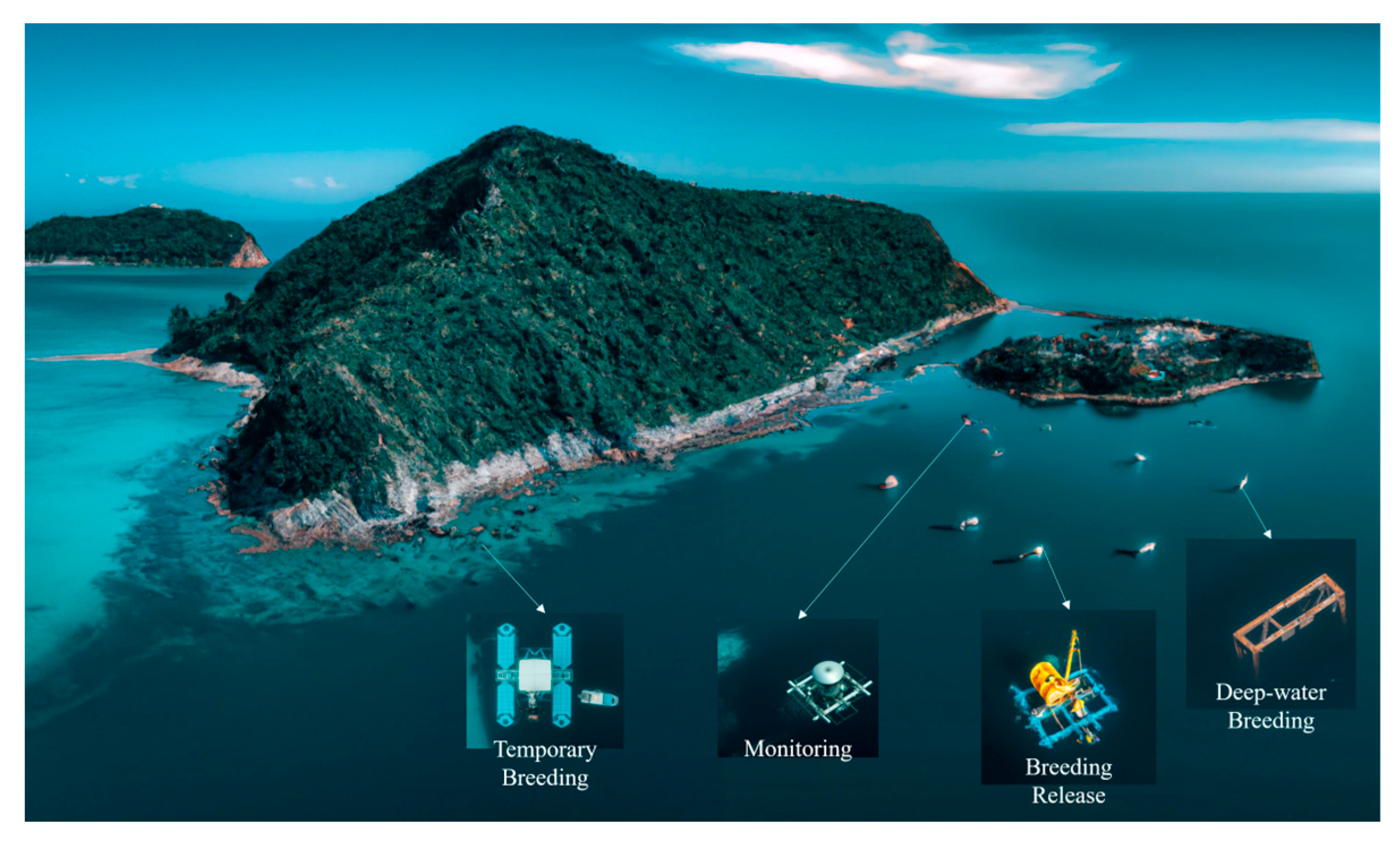
To address the above issues, this paper retains the advantages of the traditional expert system construction method and summarizes the risk and disaster types that may be encountered in the construction of marine ranches like Figure 1. It abstracts the environmental rules of the ranch environment and the risk and disaster factors and constructs a simulator of the marine ranch area’s environment. This simulator serves as an environment for interacting with intelligent agents. If the equipment deployed in the ranch is a self-cruising device, the device itself can act as the decision-making intelligent agent. Otherwise, the near-shore emergency rescue team can be set as the decision-making intelligent agent. At the same time, depending on the number of individuals available for decision making, the corresponding model-based single intelligent agent or multi-intelligent agent algorithm is selected. Through multiple rounds of policy learning and data sampling, decision-making strategy goals can be verified and optimized.

This paper proposes a decision-making model for risk and disasters in ocean ranching using reinforcement learning algorithms. We first provide an overview of the background information on the challenges associated with risk and disaster decision making in ocean ranching and the use of reinforcement learning in similar real-world scenarios. Section 2 outlines the materials and methods used to construct the model, including a discussion of the Markov Decision Processes (MDP) [13] and Partially Observable Markov Decision Processes (POMDP) [15] as well as definitions of key reinforcement learning elements. The section also provides an overview of the reinforcement learning algorithms we applied. Section 3 details the feasibility of constructing the Aquafarm model and Section 4 presents an analysis of the efficiency of various reinforcement learning algorithms in the context of the model. Finally, Section 5 and Section 6 conclude the work with a discussion of the findings as well as potential future applications and economic benefits of the proposed model.

2. Model

Reinforcement Learning (RL) is a computational algorithm used by Agents to maximize rewards while interacting with complex and uncertain Environments. The Environment receives the current state output of the Agent as an Action, and the Agent obtains a status known as a State. The feedback signal obtained by the Agent from the Environment is referred to as the Reward, and it determines whether the Agent receives a reward after taking a specific strategy in a particular step.

In Section 2 of the paper, the construction of the model is presented. This includes an explanation of the Markov Decision Processes (MDP) and Partially Observable Markov Decision Processes (POMDP) as well as definitions of essential elements in reinforcement learning.

2.1. Environment

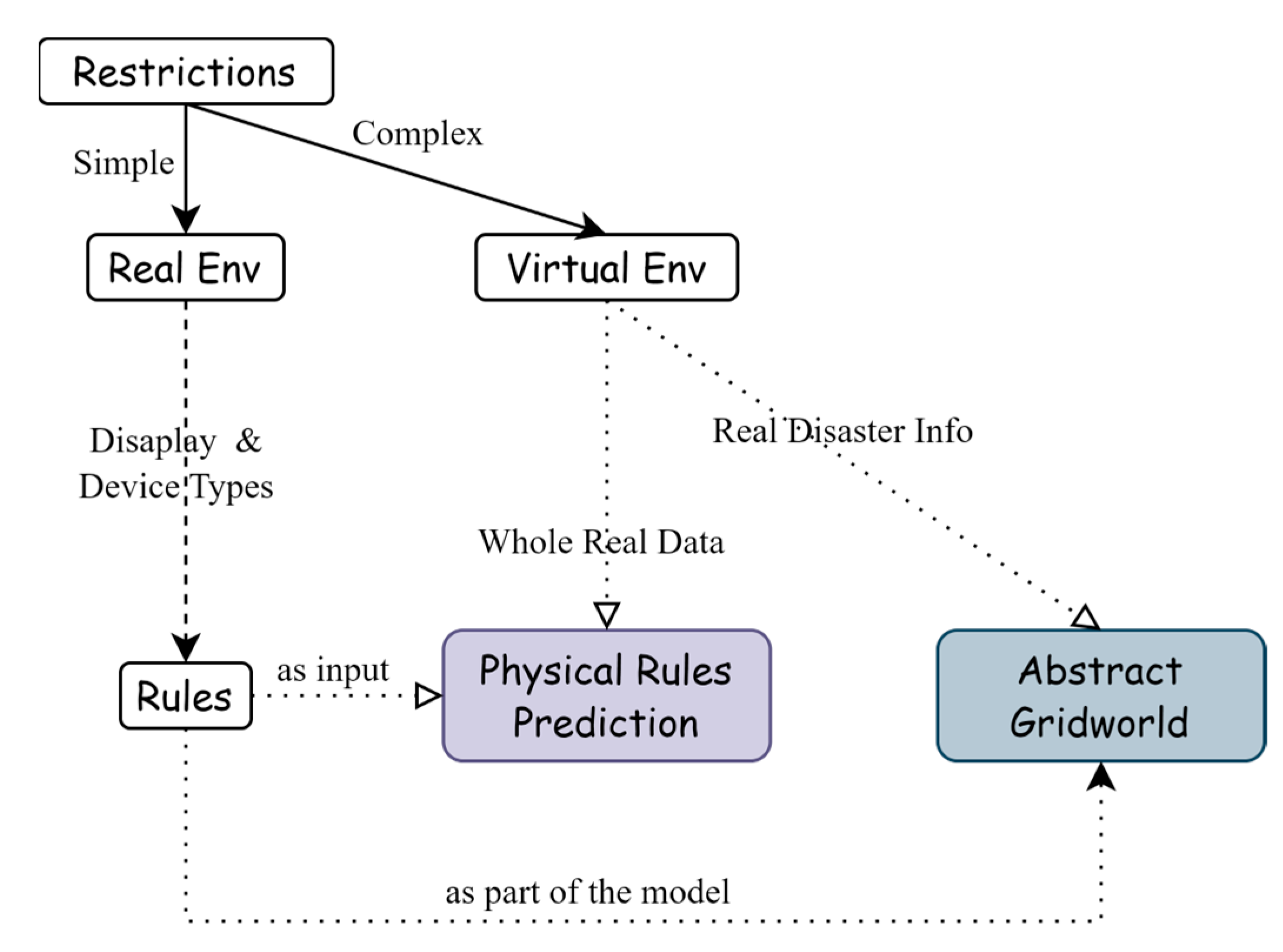
In reinforcement learning, the choice between using a real environment or a model depends on several factors, such as the complexity and cost of the environment, the availability of data, and the accuracy of the model. In some cases, it may be more feasible to use a model instead of the real environment, particularly when the real environment is too expensive or too dangerous to interact with directly. However, models can be inaccurate, and the performance of the learned policy may not generalize well to the real environment. On the other hand, using the real environment may provide more accurate feedback, but it may require more data and may be subject to safety concerns. Ultimately, the choice between using a real environment or a model depends on the specific requirements of the problem and the available resources refer to Figure 2.

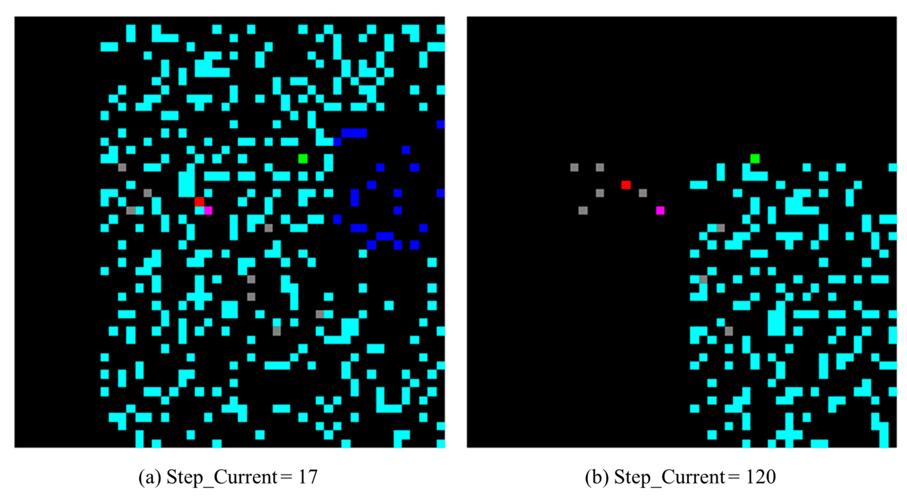
In this study, the environment consists of a grid world with rocks, locations for the squad agent(s), and devices, and another grid world with moving disaster(s). This includes defining the number of devices, ports, and agents in the system. To represent the risks or disasters, we define the disaster information class, which includes the grading level, ascending radii tuple, descending risks tuple, movement speed, and initial movement direction. We set the map size to represent the pasture located on the map, and a set of ports as the starting point of the squad and the destination of both the squad and the devices. To simulate the presence of reefs in the real marine environment, we generate a random number of rocks in the remaining blank areas on the map, each with a corresponding negative reward value. If there are islands, we can define the minimum connected area for the corresponding ports as rocks. Similarly, we randomly generate the location of the devices in the remaining positions on the map and apply the corresponding positive feedback rewards to accommodate differences in the form of different device placements, distribution forms, etc.

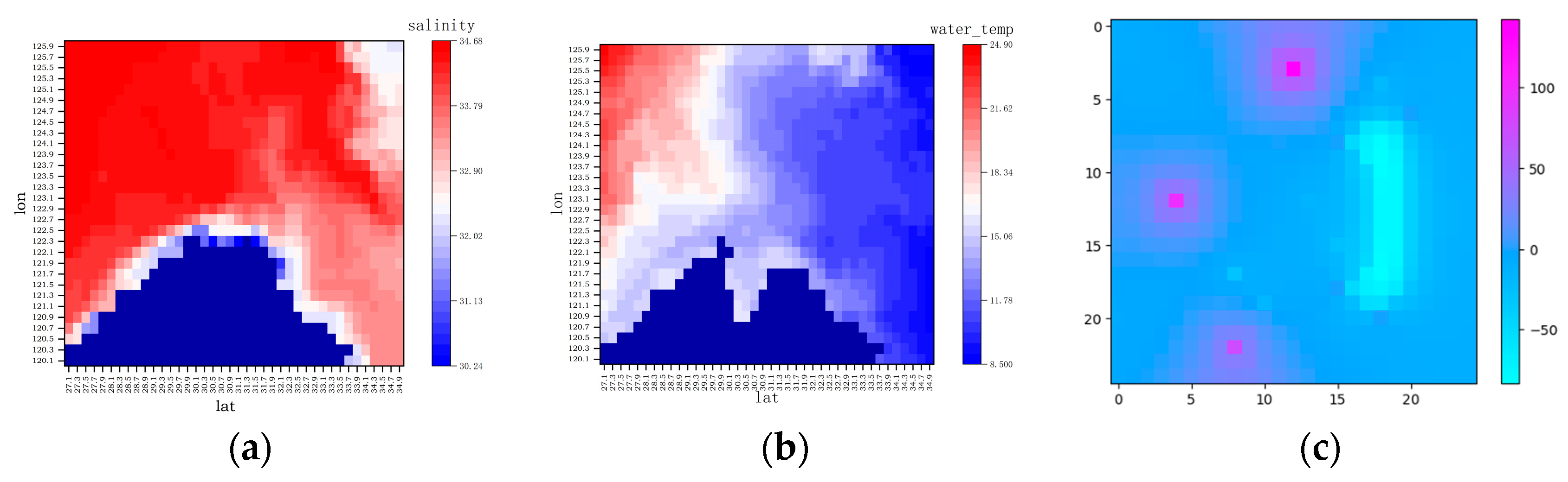
To create the disaster map to simulate the generation of impact ranges that are consistent with key information about the actual risk hazard, we enlarge the disaster map by the maximum radius value in all directions around the center of the environment map. We then use a function to randomly select a point on the disaster map as the center of the disaster.

In order to effectively train the RL agent for a disaster response in aquafarm environments, it is important to consider the different conditions that can cause an episode to terminate. In this model, we have defined two termination conditions and one truncation condition. Termination 1 occurs when all necessary equipment has been retrieved from the island, indicating a successful disaster response effort. Termination 2 occurs when the duration of the disaster has ended, which can be determined by a pre-defined time limit or external factors. These termination conditions are crucial for accurately simulating real-world disaster scenarios and for encouraging the agent to learn effective response strategies.

To simulate the generation of impact ranges that are consistent with key information about the actual risk hazard, we create the $Disaste{r}_{info}$ tuple. This involves abstractly transforming the trusted risk disaster information released by the authority into a disaster information tuple, which includes information such as the impact scope, location, distribution, and other relevant details.

In order to generate a disaster map that accurately reflects real-world disaster information, we enlarge the disaster map by the maximum radius value in all directions around the center of the environment map. We then use a function to randomly select a point on the disaster map as the center of the disaster. During each episode, the duration of the disaster is monitored, and if the episode length exceeds a certain threshold, a truncation signal is sent to the agent indicating the need to reset the environment to prevent the agent from continuing in an unproductive state.

By carefully considering, implementing, and defining these termination and truncation conditions and creating the “disaster info” element, we are able to design appropriate strategies for managing these scenarios in an aquafarm risk-and-disaster scenario model.

Algorithm 1 illustrates the sequential steps involved in setting up the environment for the aquafarm risk-and-disaster scenario model. The steps include defining the number of devices, ports, and agents; generating random rocks and devices on the map; creating a disaster map with a defined center; and defining the disaster information class. These steps are crucial in setting up an accurate and realistic environment for the reinforcement learning algorithms to learn from. The innovation of the model lies in its ability to abstract the ranch environment and to simulate disaster scenarios using real disaster information.

Algorithm 1 AquaFarm Env Model.

1: Initialize environment variables 2: Initialize Ship, Device and Port classes 3: Procedure RESET 4:   Initialize locations of ships, devices and ports 5:   Initialize environment state 6:   Generate disaster/risk 7:   return observation space 8: Procedure STEP(action) 9:   Update the position of the disaster/risk 10:   if action is a movement then 11:     Move ship 12:   else if action is operating the device then 13:     Take or drop device 14:   Update ship reward (based on the risk and crash) 15:   Update observation 16:   Add timesteps 17:   if $timesteps\ge max steps$ then 18:     Set $done=True$ 19:   return observation, reward, done and info 20: Procedure render (mode) 21:   if mode equals to “rgb_array” then 22:     return an RGB array of environment 23:   else if mode equals to “human” then 24:     Display environment 25:   else 26:     Raise an error

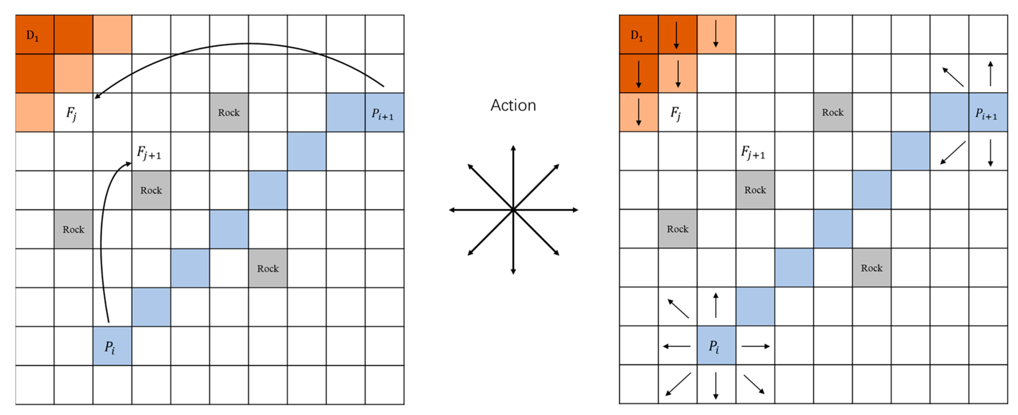
2.2. Action Space

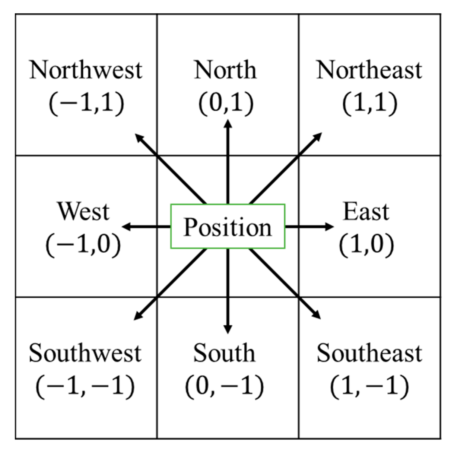
In reinforcement learning, the action space is a crucial aspect of designing an effective agent. In the case of the aquafarm environment, it is important to consider all the possible directions of movement for the squad agent like Figure 3.

$$\begin{gathered} actions=\{“N”: \left(0,1\right), “S”:\left(0,-1\right), “W”:\left(-1,0\right), “E”:\left(1,0\right), \\ “NW”:\left(-1,1\right), “NE”:\left(1,1\right), “SW”:\left(-1,-1\right), “SE”:\left(1,-1\right)\} \end{gathered}$$

(1)

Additionally, we may incorporate actions for picking up and dropping off equipment. Along with the eight directions mentioned earlier, these actions can be represented as integers within the range {0, 9}.

• 0–7: Move (8 directions)
• 8: Pickup equipment
• 9: Drop off equipment

2.3. MDP and POMDP

Constructing a Markov Decision Process (MDP) model [13] is a crucial process for developing decision-making systems in various domains such as healthcare, finance, and robotics. The MDP provides a formal mathematical framework for decision making in uncertain and dynamic environments.

To construct a model $MDP=\left(S,A,T,R,\gamma \right)$, the first step is to define the state space as $S=\left\{s_1,s_2 ,\dots , s_n\right\}$, the action space as $A=\left\{a_1, a_2, \dots , a_m\right\}$, and the reward function as $R\left(s, a\right)$. The state space represents all possible environmental states at a particular time, while the action space encompasses all feasible actions that an agent can take in a given state. The reward function maps a state–action pair to a scalar reward value.

$$G_t=R_{t+1}+\gamma R_{t+2}+{\gamma }^2{R}_{t+3}+{\gamma }^3{R}_{t+4}+\cdots +{\gamma }^{T-t-1}{R}_T$$

(2)

The discount factor is used to avoid infinite rewards in some Markov processes and to attenuate future rewards to prioritize current rewards in decision making. Its value is usually 0.99 and can be adjusted for different scenarios, with 1 meaning no discount and 0 meaning that only immediate rewards are considered.

$$\left\{\begin{array}{c}\gamma =0, ignore all the future rewards\\ \gamma =1, never discount the future rewards \end{array}\right.$$

(3)

After defining these elements, the transition function must be defined, which describes the probability of moving from one state to another after taking a specific action. The transition function is typically represented as a transition matrix $T=\left\{P_{ij}\right\}$, where $P_{ij}=p\left(s_j=s^{\prime }\mid s_i=s\right)$ signifies the probability of transitioning from state $i$ to state $j$ after taking a specific action.

$$\mathrm{T}=\left[\begin{array}{cccc}P\left(s_1\mid s_1\right)& P\left(s_2\mid s_1\right)& \dots & P\left(s_N\mid s_1\right)\\ P\left(s_1\mid s_2\right)& P\left(s_2\mid s_2\right)& \dots & P\left(s_N\mid s_2\right)\\ ⋮& ⋮& \ddots & ⋮\\ P\left(s_1\mid s_N\right)& P\left(s_2\mid s_N\right)& \dots & P\left(s_N\mid s_N\right)\end{array}\right]$$

(4)

When a state transition is Markovian, it implies that the succeeding state of a given state relies solely on its present state and is uninfluenced by any of its preceding states.

$$p\left(s_{t+1}=s^{\prime }\mid s_t=s,\dots ,s_{t=0}=s_0\right)=p\left(s_j=s^{\prime }\mid s_i=s\right)$$

(5)

The next step is constructing the environment, which embodies the dynamics of the system and includes all constituents that affect the state of the system. The final step in constructing an MDP model is to define a policy matrix. Mathematically, the policy matrix is usually $\pi =\left\{{\pi }_i\left(a\right)\right\}$, where ${\pi }_i\left(a\right)$ denotes the probability of taking action $a$ in state $i$.

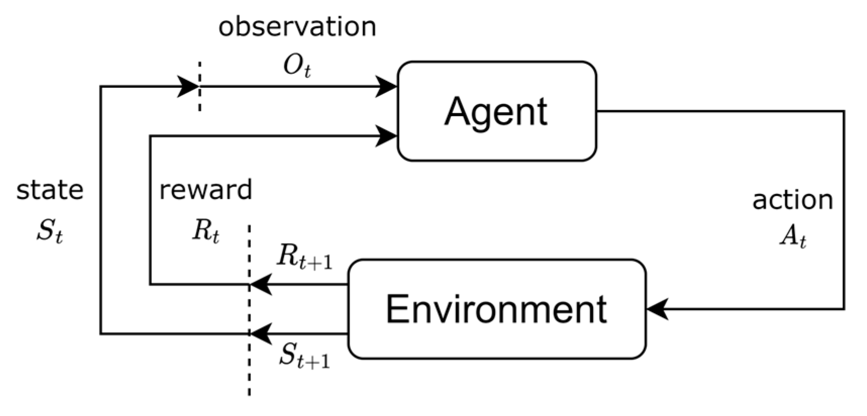
It is evident in Figure 4 that the environment updates the state, and the agent applies action to update the new state. The state $S_t$ is a complete description of the world, without hiding any information. Observations $O_t$, on the other hand, are partial descriptions of the state and may miss some information. When the agent can observe all the states of the environment as $O_t=S_t$, reinforcement learning is usually modeled as an MDP problem.

However, when the agent can only observe part of the observation, the environment is considered partially observable, and reinforcement learning is modeled as a POMDP (Partially Observable Markov Decision Processes) problem [15]. POMDP is a generalization of MDP, where the agent is assumed to be unable to perceive the environment’s state and can only know part of the observation.

$$POMDP\prime s tuple=(S,A,T=p(s^{\prime }|s,a),R,\mathsf{\Omega }=p(\mathrm{o}|\mathrm{s},\mathrm{a}), O,\gamma )$$

(6)

Under the aquafarm risk or disaster scenarios, the ocean environment is partially observed naturally, which makes it suitable for constructing a POMDP. In this case, the agent may only perceive limited environmental information collected by sensors and not have access to all the information about the ocean environment, such as the exact location of fish or the presence of predators. Therefore, the agent needs to use the available observations to infer the state of the environment and to make decisions accordingly. The construction of a POMDP model can help the agent to account for the uncertainty and partial observability of the environment and to make optimal decisions under these conditions.

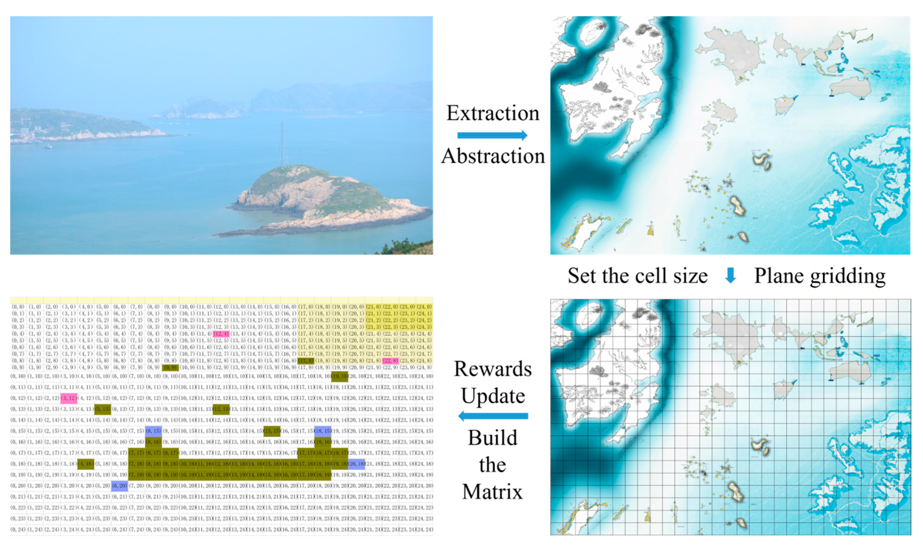
2.4. State/Observation Space

Typically, the most diminutive movable area of ranch farming equipment serves as the fundamental size of the abstract grid as Figure 5. In this experiment, it is abstracted into a 25 × 25 grid size. In this problem, the size of the state space depends on the agent’s position, the position and state of the devices, and whether the agent has picked up a device and returned it to the starting point.

Therefore, the size of the state space is: $\left|S\right|=\left(25\ast 25\right)\ast \left(2^3\right)\ast 4=128,000$, where $25\ast 25$ represents the possible positions of the agent in the grid space, $2^3$ represents the states of 3 devices (picked up or not picked up), and 4 represents the possible starting points of the agent.

The size of the observation space depends on the information that the agent can observe. If the agent can observe the entire grid space, then the size of the observation space is: $\left|O\right|=\left(25\ast 25\right)\ast \left(2^3\right)=32,000$, where $25\ast 25$ represents the possible positions of the agent in the grid space, and $2^3$ represents the states of 3 devices (picked up or not picked up).

2.5. Reward

In the aquafarm scenario, each timestep incurs a reward of −1. A crash results in each rock having a negative reward and the damage rate being proportional to the probability multiplied by the feedback value. Successfully picking up a device rewards the agent with +50. The disaster-affected area carries a negative reward, and staying in this area causes the reward to decline. Additionally, each device has a positive reward determined by its health percentage. When the agent returns to the port with a device, the reward received is the device’s status multiplied by the positive set reward. It is important to note that crashes may damage the devices on the agent, with the damage rate being equal to the rock’s negative reward divided by 100.

Reward-setting example:

• Each step (unless other reward is triggered): $-1$
• Rock: $\left[-5,-1\right]$
• Island Rock: $-20$
• Device: $\left[50, 100\right]$
• Disaster: $\left[-20,-5\right]$
• Pickup: $20$
• Drop-off device on ports: $20$
• Execute “pickup” and “drop-off” actions illegally: $-10$

2.6. Episode

The episode ends if the following happens, and the model returns the end signal:

• Termination 1: all equipment has been retrieved from the island.
• Termination 2: the duration of the disaster has ended.
• Truncation: episode length exceeded.

3. Materials and Methods

The aquafarm domain problem is a new reinforcement learning task where a squad agent must operate in a dynamic grid-world environment to achieve the task of equipment retrieval. The agent’s objective is to accomplish this task as efficiently as possible while adhering to the environment’s rules, which is similar to the taxi domain problem [16], where the agent must navigate a city grid world to pick up and drop off passengers. Both scenarios require the agent to receive rewards and penalties based on their actions and must learn how to maximize their cumulative reward over time.

However, the aquafarm problem stands out due to its dynamic nature, with the possibility of disasters occurring, which adds an additional layer of complexity. It adds additional challenges, such as the negative rewards associated with crashes and disasters as well as the varying health statuses of equipment that must be taken into account. While describing the method and policy of agent construction, a synopsis of well-known reinforcement learning algorithms is also provided, including Q-Learning, SARSA, and both the basic and LSTM versions of DQN.

3.1. Agent

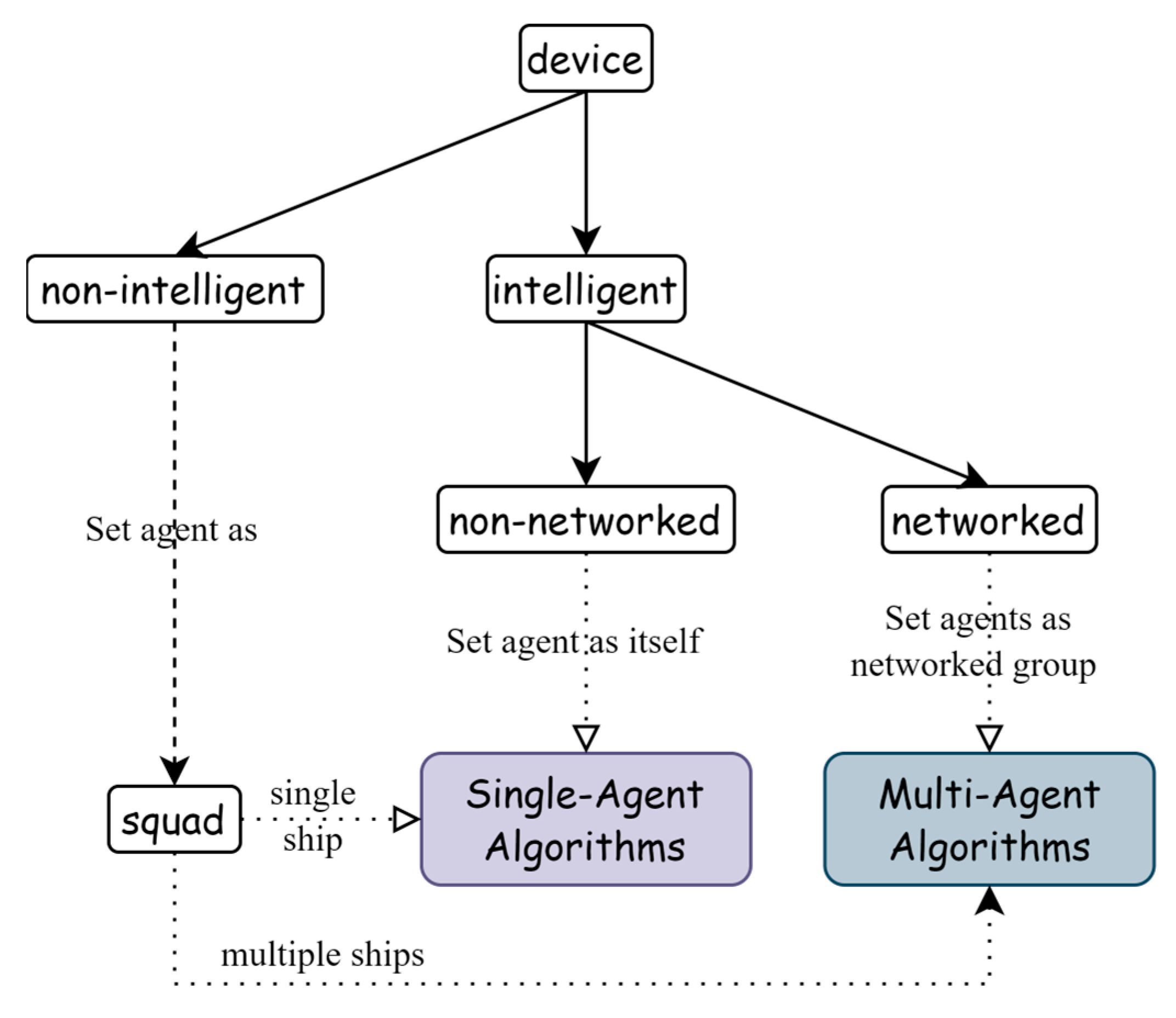
When designing a reinforcement learning system for marine ranching, it is essential to carefully consider the agent element based on the available resources and specific goals refer to Figure 6. Select single or multi-intelligent agent algorithms based on device characteristics, number, and other specifics. For non-intelligent equipment, such as those without autonomous capabilities, a near-shore rescue and relief squad can be set as the agent. For intelligent equipment, the device itself can be the agent, and a single intelligent agent reinforcement learning algorithm can be used for each device.

However, a multi-agent algorithm may be needed when the smart devices are networked together or there is more than one squad, and a higher level of coordination is required. A multi-agent reinforcement learning (MARL) system, consisting of agents interacting to achieve a common goal, may be necessary. In such systems, value-based algorithms or policy-based algorithms can be used. The number of agents required should also be considered, as it greatly affects system performance. In our experiments, we used a value-based algorithm called Multi-Agent Deep Deterministic Policy Gradient (MADDPG) [17] for cooperative MARL problems. MADDPG is a decentralized algorithm that allows each agent to learn its policy independently while also considering the policies of other agents through a centralized critic.

Careful consideration of the type and number of agents used in a reinforcement learning system is crucial in designing an effective and efficient system for decision making in marine ranching.

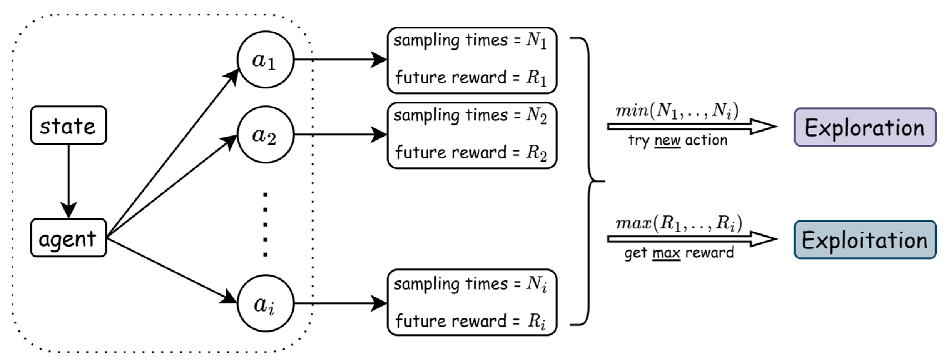
3.2. Exploration/Exploitation

Reinforcement learning (RL) algorithms typically face a trade-off between exploration and exploitation shows in Figure 7. Exploration involves taking actions that the agent has not attempted before, whereas exploitation involves taking the best-known action based on previous experiences.

One way to balance exploration and exploitation is epsilon–greedy, where the agent takes the best-known action with a probability of $1-\epsilon$ and a random action with a probability of $\epsilon$.

$$a=\left\{\begin{array}{c}arg\underset{a}{\max }Q\left(s,a\right), with probability 1-\epsilon \\ random, with probability \epsilon \end{array}\right.$$

(7)

Similarly, the Boltzmann exploration strategy [18] generates a probability distribution over actions using a SoftMax function, where the temperature parameter controls the degree of exploration.

$$P\left(a|s\right)=\frac{\exp \left(Q\left(s,a\right)\right)}{{{\displaystyle \sum }}_a\exp \left(Q\left(s,a\right)\right)}$$

(8)

In addition, Intrinsic Curiosity Models [19] aim to address exploration by encouraging the agent to explore novel and uncertain environments through intrinsic rewards. In terms of similarities, all three methods seek to address the exploration–exploitation dilemma in RL. However, they differ in the degree of randomness they introduce to the agent’s actions, the form and source of the exploration signal, and the computational cost associated with their implementation.

Epsilon–greedy is the simplest method, while Boltzmann exploration introduces an additional parameter that must be tuned. Finally, intrinsic curiosity models require more computation and resources but generally result in higher-quality exploration.

3.3. Policy

In the context of Markov Decision Processes (MDPs), a policy is a function that maps states to probability distributions over actions. Specifically, a stationary policy is a policy that is independent of time and remains fixed throughout an episode. The probability of selecting action $a$ in state $s$ under policy $\pi$ is denoted as $\pi (a|s)$.

$$\pi \left(a|s\right)=P\left(A_t=a|S_t=s\right)$$

(9)

A stationary policy, when followed in an MDP, gives rise to a Markov Reward Process (MRP) that is characterized by the tuple $M=\left(S,P,R,\gamma \right)$, where $S$ is the state space, $P$ is the transition probability function, $R$ is the reward function, and $\gamma$ is the discount factor. An MRP is a stochastic process that describes the evolution of a state and a reward over time. The value function of a stationary policy $\pi$, denoted as $V_{\pi }\left(s\right)$, is the expected sum of discounted rewards obtained from following policy $\pi ,$ starting from state $s$.

$$V_{\pi }\left(s\right)={\displaystyle \sum }_a\pi (a|s){\displaystyle \sum }_{s^{\prime }}(s^{\prime }|s,a)\left[R\left(s,a,s^{\prime }\right)+\gamma V_{\pi }\left(s^{\prime }\right)\right]$$

(10)

The optimal policy in an MDP is the policy that maximizes the expected sum of discounted rewards. It is denoted as ${\pi }^{*}$. The optimal value function, denoted as $V^{*}$, is the maximum value function over all possible policies. The optimal value function satisfies the Bellman optimality equation, which is a recursive equation that relates the value of a state to the values of its successor states.

$$V^{*}\left(s\right)=\underset{a}{max}\sum _{s^{\prime }}P\left(s^{\prime }\mid s,a\right)\left[R\left(s,a,s^{\prime }\right)+\gamma V^{*}\left(s^{\prime }\right)\right]$$

(11)

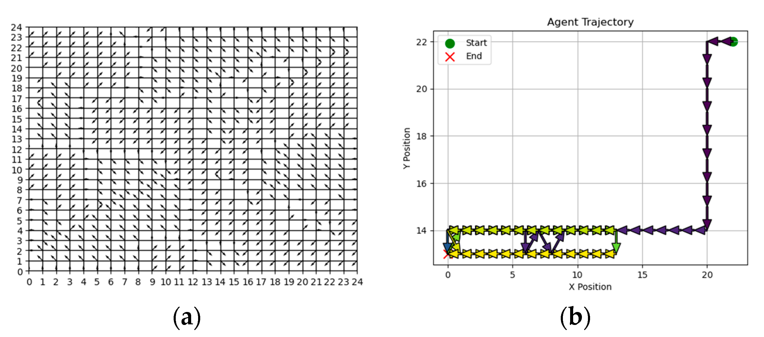
In the context of our aquafarm risk-and-disaster scenario model, we will use reinforcement learning to learn an optimal policy that maximizes the expected cumulative reward over a finite horizon. The policy will be learned through an iterative process of interacting with the environment and adjusting the policy parameters based on the observed rewards. The objective of the learned policy will be to minimize the risk of loss in the aquafarm due to disasters while maximizing the overall profit.

When the agent is set to a near-shore rescue and relief squad, the navigable port location is set as the starting and ending sequence, and a single intelligent body or multi-intelligent body algorithm is chosen according to the number of squads. When the agent is the device itself, a single-intelligent body reinforcement learning algorithm is used for each device, regardless of the number of devices in the pasture; when the intelligent device is between the device network, a multi-intelligent body algorithm can be used.

3.4. Algorithm Formulas

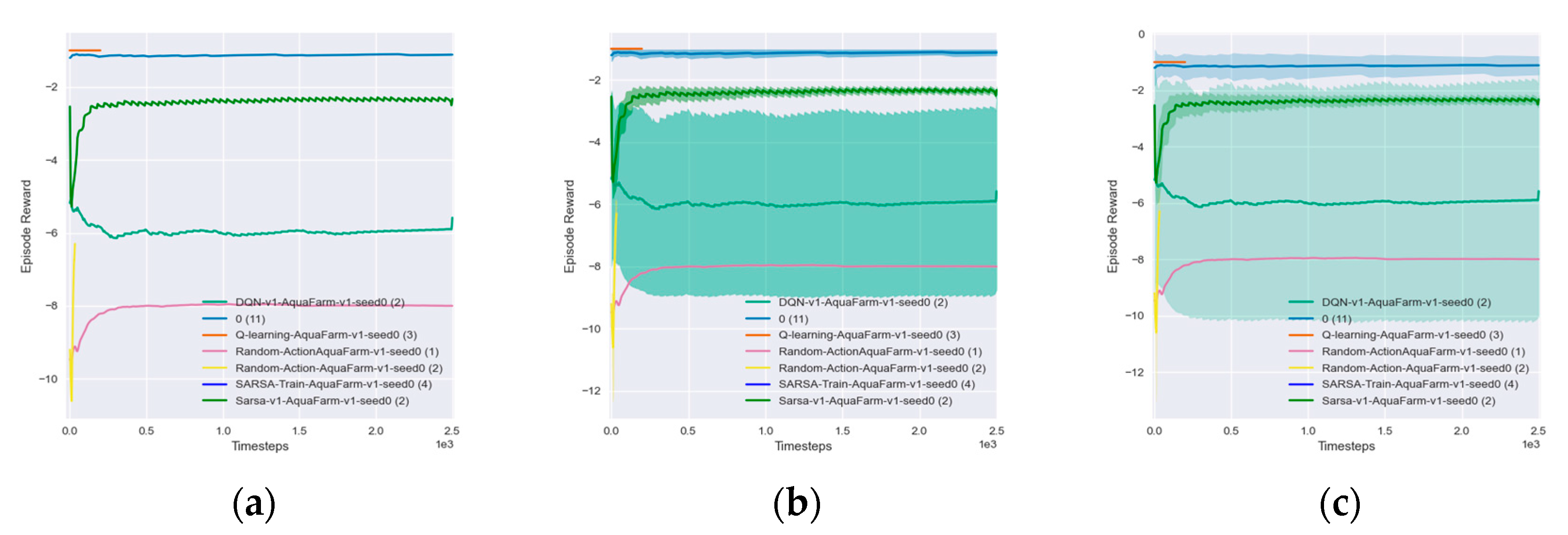
Our focus is on value-based algorithms due to their superiority over policy-based algorithms in our experiments. Value-based algorithms are more stable, simpler, and perform better than policy-based algorithms. These algorithms estimate the optimal value function, which represents the expected total reward an agent can receive from a given state. The experiment in our paper aims to compare and evaluate the performance of four reinforcement learning algorithms: Q-learning [20], SARSA [21], DQN [22], and the DQN algorithm with Long Short-Term Memory (LSTM).

3.4.1. Q-Learning

The Q-learning algorithm is a widely recognized approach to reinforcement learning and was first introduced by Watkins in 1989. The fundamental concept behind Q-learning is the approximation of the optimal action–value function, denoted as the Q-function, which links each state–action pair to the anticipated discounted future reward.

$$Q\left(s,a\right)=Q\left(s,a\right)+\alpha \left[r+\gamma max\left(Q\left(s\prime ,a\prime \right)\right)-Q\left(s,a\right)\right]$$

(12)

where $\alpha$ is the learning rate ($0<\alpha \le 1$), $\gamma$ is the discount factor ($0\le \gamma <1$), and $\max \left(Q\left(s\prime ,a\prime \right)\right)$ is the maximum Q-value for the new state $s’$ over all possible actions $a’$. Q-learning employs an iterative update scheme to update the Q-values of state–action pairs based on the perceived reward signal and the maximum Q-value of the next state. The Q-function satisfies the Bellman equation:

$$Q(s,a)=\mathbb{E}\left[r+\gamma \underset{a^{\prime }}{\max }Q\left(s^{\prime },a^{\prime }\right)\mid s,a\right]$$

(13)

However, Q-learning can be slow to converge when the state and action space are large, and it can be difficult to scale to high-dimensional inputs.

3.4.2. SARSA

The SARSA algorithm’s performance may be better than Q-learning because it considers the maximum reward in the current state as well as the next action.

$$Q\left(S_t,A_t\right)\leftarrow Q\left(S_t,A_t\right)+\alpha \left[R_{t+1}+\gamma Q\left(S_{t+1},A_{t+1}\right)-Q\left(S_t,A_t\right)\right]$$

(14)

It may be better able to avoid falling into a local optimal solution than the Q-learning algorithm. In experiments, we may observe that the average reward and success rates of the SARSA algorithm are higher, but it may converge at a slightly slower rate.

3.4.3. Deep Q-Network (DQN)

DQN (Deep Q-Network) is a popular reinforcement learning algorithm that uses a neural network to approximate the Q-function. The DQN algorithm uses an experience-replay buffer to store the experiences, which are randomly sampled during training. This helps to break the correlation between consecutive updates and improves the stability of the algorithm. It also uses a target network, which is a copy of the Q-network that is used to generate the target Q-values during training. The target network is updated less frequently than the Q-network to improve stability. The loss function used in the DQN is the mean squared error between the predicted Q-value and the target Q-value, which is calculated as:

$$L_i\left({\theta }_i\right)=\mathbb{E}s,a,r,s^{\prime }[\left(r+\gamma \underset{a^{\prime }}{\max }Q\left(s^{\prime },a^{\prime };{\theta }_i^{-}\right)-Q\left(s,a;{\theta }_i\right){)}^2\right]$$

(15)

The DQN algorithm can handle continuous states and action spaces and outperforms the previous two algorithms in terms of average return and success rate, but it may converge more slowly.

3.4.4. Deep Q-Network (DQN)-Based LSTM (Long Short-Term Memory)

In this study, we developed a DQN algorithm with a long short-term memory (LSTM) model, which will be tested in the general disaster scenario and used to construct the decision algorithm.

In Algorithm 2, the pseudocode shows the entire process of implementing the algorithm and the application formula, where the mathematical symbols refer to the variables and their meanings, which are described in the pseudocode or in the previous section.

Algorithm 2 DQN with LSTM.

1: Procedure Initialization of Deep Q-Network with LSTM 2:   Initialize the replay memory $D$ with capacity $N$ 3:   Initialize the batch size $B$ and the quantity of epochs $E$ 4:   Initialize the LSTM network parameter $\theta$ with random weight $\omega$ 5:   Initialize the target LSTM network parameter ${\theta }^{-}$ with the same $\omega$ 6:   Initialize the LSTM cell state $c_{t=0}$ and hidden state $h_{t=0}$ to zero 7:   Initialize the exploration rate $\epsilon$ and the minimum ${\epsilon }_{min}$ in $\left[0,1\right]$ 8:   Initialize the discount factor $\gamma$ in $\left[0,1\right]$ 9:   Initialize the length of sequences $L$ in $\left[1,N\right]$ 10:   Initialize the state $s_{t=0}$ by pre-processing the initial environment 11: Procedure Training 12:   for $t$ in $\left[1,N\right]$ do 13:     $a_t=\left\{\begin{array}{c}arg\underset{a}{\max }{Q}^{\theta }\left(s_t,a,c_{t-1},h_{t-1}\right), with probability 1-\epsilon \\ random, with probability \epsilon \end{array}\right.$ 14:     receive reward $r_t$ and next state $s_{t+1}$ 15:     append the tuple $\left(s_t,a_t,r_t,s_{t+1}\right)$ to $D$ 16:     if $\left|D\right|>N$ then 17:       remove the oldest tuple from $D$ 18:     if $t>L$ then 19:       Sample a minbatch of tuples $\left(s_j,a_j,r_j,s_{j+1}\right)$ from $D$ 20:       compute target value $Y_j=\left\{\begin{array}{c}{r}_j, terminates at step j\\ r_j+\gamma \underset{a}{\max }{Q}^{{\theta }^{-}}\left(s_{j+1},a,c_j,h_j\right),other\end{array}\right.$ 21:       update $\theta$ by MSE: $\mathcal{L}\left(\theta \right)=\frac{1}{B}{\displaystyle \sum }_{j=1}^B{\left[Y_j-Q^{\theta }\left(s_j,a_j,c_{j-1},h_{j-1}\right)\right]}^2$ 22:       update ${\theta }^{-}$: ${\theta }^{-}\leftarrow \tau \theta +\left(1-\tau \right){\theta }^{-},hyper-paramter \tau \in \left[0,1\right]$ 23:     update $\epsilon$ according to a specified schedule

The LSTM model is a recurrent neural network (RNN) model for time-series data processing that captures long-term dependencies in time-series data and incorporates historical data into the modeling. Each unit has a forgetting gate and an updating gate to control when to remember or forget the previous state.

4. Results

4.1. Aquafarm Model

The reinforcement learning-based simulation model to improve decision-making capacity and efficiency in response to aquaculture risk and disaster scenarios aims to provide a safe, cost-effective, and scalable way to test and refine disaster response strategies in aquaculture environments. The model simulates various disaster scenarios and evaluates the effectiveness of different response strategies, enabling aquafarm operators and disaster response agencies to develop and test response strategies without incurring the costs and risks of real-world disasters.

Our paper introduces a novel approach for developing a risk-and-disaster scenario model for aquafarming through reinforcement learning. As described in Figure 8, we abstracted the sea environment into a grid model and utilized it as an interactive environment to determine the bonus value of the key components in the ranch sea area, ultimately updating the grid environment accordingly.

4.1.1. Simulation of Disaster Movement

After the rewards are set for the main components in the marine, the model will update the grid matrix. Simultaneously, the simulated disaster moves in a certain direction from time to time. Below are the outputs of the grid at different times during the training refer to Figure 9: the left (a) shows the execution of step 17 while the right (b) shows the execution of step 120 in one episode.

4.1.2. Simulation of Disaster Distribution

To validate our method’s feasibility, we compared the value matrix $V_{\pi }$ obtained from our model with the historical data collected by the equipment in the form of a heat map. The results refer to Figure 10 demonstrate that our model can accurately simulate the risk and disaster scenarios in terms of the structure and form of distribution.

In summary, the results show that the Aquafarm model is fundamentally capable of stimulating both the distribution and the motions of catastrophes and demonstrate the potential of the application of reinforcement learning to build a scenario model of aquaculture within a grid environment that is abstract enough to train reinforcement learning agents.

4.2. Algorithm Evaluation Metrics

In this study, we evaluated the performance of three commonly used reinforcement learning algorithms, namely Q-learning, SARSA, DQN, with the baseline of the RANDOM algorithm. In the experiment, the RANDOM algorithm means that a fully unlearned agent, chooses each action within the choice reachable (for example, except reefs, islands, etc.) with equal probability and randomly samples one action at a time to serve as the baseline or benchmark for this experiment like Figure 11.

Our findings in Figure 12 indicate that Q-learning and SARSA have lower average returns compared with DQN, as they require more iterations to converge to optimal policies. Additionally, Q-learning has a lower success rate than SARSA, while DQN has the highest success rate due to its ability to learn from large state spaces and to use experience replay to improve stability.

Regarding convergence speed, our results in Figure 13 indicate that SARSA had a faster convergence speed than Q-learning due to its ability to learn from on-policy experience and to converge to a local optimum faster. DQN had the fastest convergence speed compared with Q-learning and SARSA, as it utilized a deep neural network to approximate the action–value function and could learn from large state spaces.

Finally, our study evaluated the stability of the algorithms, in Figure 14 which indicated that Q-learning was less stable than SARSA due to its tendency to not converge to optimal policy in some situations. SARSA was found to be more stable than Q-learning, while DQN was found to be the most stable due to its trained deep neural network.

To compare their effectiveness more explicitly, we measured and analyzed the following evaluation metrics: average return, success rate, convergence speed, and stability. Each algorithm was experimented with 10 times, each time running 2000 episodes, with each episode allowing 5000 steps at maximum, and the average of the experiment results was considered to be the final result. Here we can define the equation of these four metrics as:

$$\begin{gathered} EA\left(alg{o}_i\right)=w_1\ast AverageReturn+w_2\ast SuccessRate+w_3 \\ \ast ConvergenceSpeed+w_4\ast Stability \end{gathered}$$

(16)

Here, $w_1$, $w_2$, $w_3,$ and $w_4$ represent the weights assigned to each metric. The evaluation process for this experiment prioritizes stability, followed by success rate, convergence speed, and average returns, in that order. To better reflect the importance of each metric, we adjust this formula based on the value of $w_1=0.1,w_2=0.3,w_3=0.2,w_4=0.4$. The higher the value of the EA equation, the better the performance; however, the four indicators cannot be directly calculated and added together to assess performance but still need to be converted, especially the convergence speed.

Table 1. Comparison of four algorithms using four evaluation metrics.

Algorithm	Average Return	Success Rate	Convergence Speed	Stability	EA(algo)
DQN with LSTM	1.67 per step	1	≤300 timesteps (4)	1	1.67
SARSA	−1	0.9	≤700 (2)	0.9	0.93
Q-Learning	−1.21	0.7	≤500 (3)	0.7	0.97
RANDOM	−10	0	Failed (1)	0	−0.7

contains the results. Retain no more than two decimal places for calculations.

These findings can inform the selection of appropriate reinforcement learning algorithms in different scenarios based on their performance characteristics. By adjusting hyperparameter variables such as the exploration rate $ϵ$, learning rate $\alpha$, discount rate $\gamma$, and $Nu{m}_{episodes}$, the performance of the algorithm can also be optimized.

5. Discussion

The study demonstrates the potential of AI in addressing the challenges of marine ranching, particularly in the area of risk and disaster management. The use of deep reinforcement learning enables the modeling of complex environmental systems and the optimization of decision-making processes, leading to the improved efficiency and sustainability of marine ranch operations. The proposed approach has significant implications for the marine ranching industry as it provides a framework for enhancing the resilience and adaptability of marine ranches to various types of risks and disasters.

However, the adoption of AI in marine ranching is not without challenges. The complexity of marine ecosystems, the variability of environmental factors, and the need for domain-specific knowledge pose significant challenges to the development and deployment of AI-based solutions in marine ranching. Furthermore, the potential social and ethical implications of AI-driven marine ranching require careful consideration, particularly with regard to issues such as data privacy, ownership, and governance.

Despite these challenges, the findings of this study highlight the potential of AI in marine ranching and the importance of continued research and innovation in this field. The development of AI-driven marine ranching has significant implications for global food security, environmental sustainability, and economic growth, particularly in countries with large coastal areas such as China.

Moreover, our model’s distinctiveness lies in its capacity to leverage actual disaster data to create simulated disaster scenarios. Our abstraction of the ranch environment and the integration of real-world information empower our model to handle unforeseen events and to offer more precise forecasts of potential hazards. In our subsequent research, we intend to delve into the adoption of sophisticated machine-learning techniques, like generative adversarial networks and transfer learning, to complement our use of deep reinforcement learning and to advance the efficacy of our aquafarm model. Furthermore, we aim to explore the applicability of our model in diverse marine ranching environments.

In summary, the proposed methodology provides a foundation for future research, and future studies could focus on refining the proposed approach, evaluating its performance, and addressing the challenges and opportunities of AI-driven marine ranching from a broader societal perspective.

6. Conclusions

This study shows the potential use of deep reinforcement learning in marine ranching, particularly in the field of risk and disaster response. The research in the two following areas is summarized here: The first area involved the use of reinforcement learning theory and Markov correlation principles to define key decision-making elements in marine ranching scenarios. It also included modeling the complex ocean environment using Aquafarm, a simulator of the ocean ranch area, to lay the foundation for reinforcement learning in ocean ranch scenarios. The second area involved the analysis of ocean ranch equipment characteristics and the creation of intelligent decision-making systems for ranching. It further included designing and implementing a strategy-learning algorithm based on Long Short-Term Memory (LSTM) for the DQN algorithm and validating the feasibility of the disaster decision-making algorithm for ranching based on deep reinforcement learning through comparative experiments based on the Aquafarm model.

In conclusion, the intelligent implementation of marine ranching, assisted by deep reinforcement learning, has optimistic prospects. However, several technical and economic challenges require resolution in practical applications to enhance its stability, efficiency, safety, and feasibility. Future research can be directed toward enhancing the method by integrating more sophisticated algorithms and models, incorporating diverse data sources and sensors, and analyzing the social and economic implications of AI-powered marine ranching. Additionally, deep reinforcement learning will play a progressively significant role in decision making for high-risk disasters at sea, as farm equipment continues to acquire more advanced features.