Interpretable Feature Construction and Incremental Update Fine-Tuning Strategy for Prediction of Rate of Penetration

Abstract

Prediction of the rate of penetration (ROP) is integral to drilling optimization. Many scholars have established intelligent prediction models of the ROP. However, these models face challenges in adapting to different formation properties across well sections or regions, limiting their applicability. In this paper, we explore a novel prediction framework combining feature construction and incremental updating. The framework fine-tunes the model using a pre-trained ROP representation. Our method adopts genetic programming to construct interpretable features, which fuse bit properties with engineering and hydraulic parameters. The model is incrementally updated with constant data streams, enabling it to learn the static and dynamic data. We conduct ablation experiments to analyze the impact of interpretable features’ construction and incremental updating. The results on field drilling datasets demonstrate that the proposed model achieves robustness against forgetting while maintaining high accuracy in ROP prediction. The model effectively extracts information from data streams and constructs interpretable representational features, which influence the current ROP, with a mean absolute percentage error of 7.5% on the new dataset, 40% lower than the static-trained model. This work provides a theoretical reference for the interpretability and transferability of ROP intelligent prediction models.

1. Introduction

Drilling operations play a crucial role in the petroleum industry, as they involve the creation of boreholes to extract valuable resources. The rate of penetration (ROP) refers to the ratio of the length of rock penetration to the corresponding drilling time. Accurate prediction of the ROP plays a vital role in drilling operations, as it directly impacts cost and efficiency. By achieving accurate ROP predictions, drilling engineers can make informed decisions in real time, optimizing drilling parameters and adjusting drilling strategies to enhance drilling efficiency and minimize operational expenses. Proper ROP prediction contributes significantly to cost effectiveness, operational efficiency and risk management in drilling activities [1].

The prediction of ROP has been extensively investigated in the petroleum industry, and two primary frameworks have been utilized: physics-based models and intelligent models. Physics-based models, including the Maurer model [2], the Galle model [3], the Bourgoyne–Young model [4], the Walker model [5], the Hareland model [6], the Detournay model [7] and the Wiktorski model [8], also known as analytical models, attempt to formulate the relationship between the ROP and influencing factors through mechanism analyses. These models have been developed over several decades, incorporating theoretical analysis, laboratory experiments and field observations. While physics-based models align with physical drilling laws and offer interpretability, they often struggle to capture the physically unclear relationships due to the intricate and unpredictable downhole environments. The inherently strong non-linearity and complexity of these relationships make it challenging to formulate them into explicit equations. Moreover, these models are often computationally intensive and require extensive input data. Consequently, their practical applicability and accuracy in the field are limited.

In recent years, driven by advances in artificial intelligence (AI), which has been widely used in many scenarios [9,10,11,12] and has gained significant attention for ROP prediction [13,14,15], many scholars have tried to use AI technology to solve complex non-linear problems in petroleum engineering. Intelligent models aim to approximate the complex relationship between the ROP and influencing factors by leveraging their powerful non-linear fitting capabilities. Artificial neural networks (ANNs) have been widely used, demonstrating promising results in ROP prediction [16,17]. Other machine-learning models, such as random forest [16,18,19], extreme gradient boosting [14,20], long and short-term memory (LSTM) networks [21,22] and hybrid networks [23,24], have been applied to predict ROP based on historical drilling data. Bizhani et al. [25] addressed the issue of uncertainty in data-driven models by developing a Bayesian neural network model for predicting ROP. Their approach revealed the fundamental reasons behind the lack of accuracy in ROP models. Pacis et al. [26] applied transfer learning to drilling speed prediction. They used a fine-tuning method to freeze the parameters of a well-trained ANN model and transfer it to train ROP prediction models for other wells. Intelligent models, while offering better accuracy and fitting capabilities compared to physics-based models, often face limitations related to data requirements and interpretability. These models typically necessitate a large amount of data to build robust and accurate algorithms. The availability of comprehensive and high-quality datasets is crucial for training intelligent models effectively. However, it is important to note that the performance of intelligent models heavily relies on the distribution of the training data. This implies that their performance may be significantly affected when applied to different test wells, potentially leading to catastrophic outcomes.

While both physics-based and data-driven models have made significant contributions to ROP prediction, several gaps in the existing research still need to be addressed. The first key aspect pertains to the multitude of factors influencing the ROP (e.g., weight on bit (WOB), rotary speed (RPM), inlet flow rate (Q), torque (T)). Generally, it is challenging for models to obtain a comprehensive set of influential features for accurate prediction. Existing data features often fall short in fully capturing the changing trends in ROP. Li and Yang [27] designed a genetic algorithm (GA)-based feature construction framework to generate interpretable features in the ironmaking process, but studies focusing on feature construction techniques for ROP prediction remain insufficient.

Secondly, intelligent models trained exclusively on historical data often encounter challenges in generalizing well to new well conditions. These models struggle to adapt to the inherent variations and complexities present in unseen drilling environments [1]. Therefore, it is crucial to incorporate new data and update model parameters incrementally to maintain accuracy and relevance. Zhang et al. [13] and Soares and Gray [18] proposed real-time ROP prediction models, which make accurate predictions by continuously learning from the latest drilling data. However, these models encounter difficulties in being robust and adaptable to handle various operational scenarios.

To address these limitations, it is essential to develop advanced prediction models, which have the ability to handle complex and dynamic drilling environments. The key contributions of this research include

• Introducing advanced feature engineering techniques to construct interpretable features, which align with the physical drilling laws.
• Developing an incremental update fine-tuning strategy to adapt the model to changing drilling conditions.
• Evaluating the performance of the proposed model and comparing it with existing approaches in terms of accuracy and adaptability.

The remainder of this paper is organized as follows. Section 2 presents the methodology, including dataset description, the details of interpretable feature construction and the incremental update fine-tuning strategy. The results and discussion are presented in Section 3, which analyzes the impact of interpretable features and incremental updating and model performance. Finally, Section 4 concludes the paper, summarizing the research contributions.

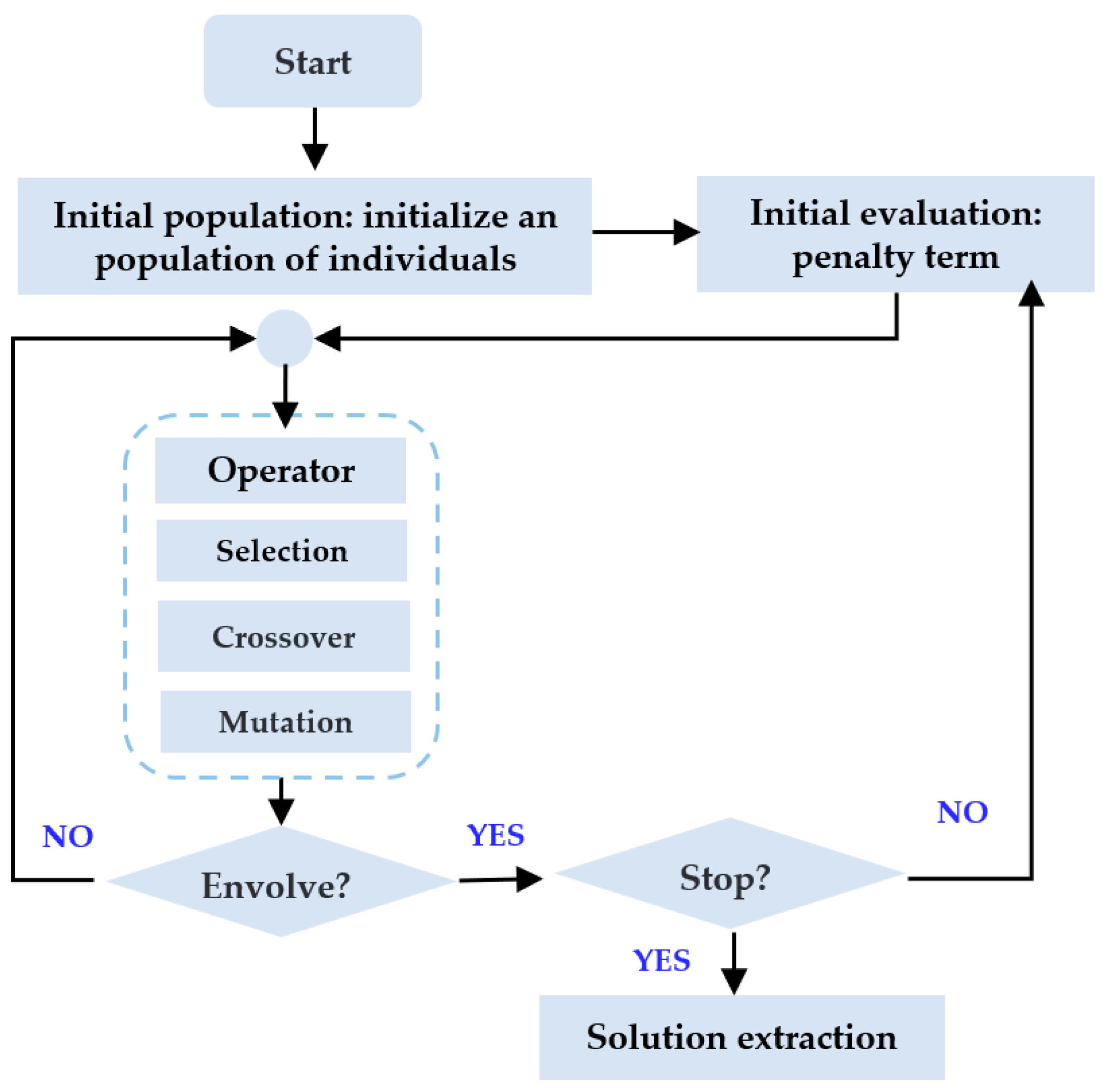
2. Methodology

In this section, we focus on processing the datasets, selecting appropriate input parameters, constructing interpretable domain features, developing an intelligent ROP prediction model and displaying the incremental update fine-tuning strategy, as shown in Figure 1.

2.1. Dataset Preparation

2.1.1. Data Pre-Processing

The data in this study were collected from eight wells in the Xinjiang Oilfield, China, including the formation properties, engineering parameters, hydraulic parameters and bit properties. To prepare a reliable dataset for model training, a data alignment operation is first required to ensure consistency and coherence of the dataset by organizing and synchronizing the different data sources. This step is critical for processing data from a variety of drilling parameters, geologic attributes and engineering factors, which may have been collected at different time intervals. Next, three times the mean standard deviation (3σ) outlier removal method is used to identify and eliminate data points that deviated significantly from the mean or expected value. Specifically, data points that exceed 3σ are considered outliers and removed from the dataset. The selection of appropriate input features plays a crucial role in the performance of intelligent models. To capture the complex factors influencing ROP, we compute the Pearson correlation coefficient [28] (ranging from −1 to 1) using the Python Pandas library, and the distance correlation coefficient [29] (ranging from 0 to 1) is implemented with our own coding. The calculation formulas of two correlation coefficients are defined as follows:

$$Pc=\frac{{\displaystyle \sum _{i=1}^n(X_i-\overline{X})(Y_i-\overline{Y})}}{\sqrt{{\displaystyle \sum _{i=1}^n{(X_i-\overline{X})}^2}}\sqrt{{\displaystyle \sum _{i=1}^n{(Y_i-\overline{Y})}^2}}}$$

(1)

$$dCor(X,Y)=\left\{\begin{array}{ll}\frac{dCo{v}_n^2\left(X,Y\right)}{\sqrt{dCo{v}_n^2\left(X\right)dCo{v}_n^2\left(Y\right)}}& dCo{v}_n^2\left(X\right)dCo{v}_n^2\left(Y\right)>0\\ 0& dCo{v}_n^2\left(X\right)dCo{v}_n^2\left(Y\right)=0\end{array}\right.$$

(2)

where X_i and Y_i are the individual data points for variables X and Y, respectively; $\overline{X}$ and $\overline{Y}$ are the mean values of variables X and Y, respectively; $dCo{v}_n^2\left(X,Y\right)$ is the distance covariance of X and Y, which is calculated as the average of the pairwise product of the distance matrices of X and Y. $dCo{v}_n^2\left(X\right)$ is the standard deviation of the distance of X, and $dCo{v}_n^2\left(Y\right)$ is the standard deviation of the distance of Y.

The calculations revealed a strong linear correlation between the inflow rate and hook load. To maintain model stability, only one of them was selected as an input, as shown in

Table 1. Two types of correlation coefficients between features and ROP. Drilling fluid viscosity here refers to the apparent viscosity of the drilling fluid, also called funnel viscosity, which is defined as the time required for a given volume of drilling fluid to flow through a small hole of a specified size.

Variables	Pearson Correlation Coefficient	Distance Correlation Coefficient
Depth (m)	0.129	0.108
Weight on bit (kN)	−0.224	0.223
Rotary speed (rev/min)	0.354	0.380
Torque (kN∙m)	0.221	0.292
Standpipe pressure (MPa)	0.349	0.323
Inlet flow rate (L/s)	−0.194	0.236
Bit drill distance (m)	0.265	0.284
Bit size (mm)	−0.236	0.266
Drilling fluid density (g/cm3)	0.419	0.413
Drilling fluid viscosity (s)	0.247	0.308
Gamma ray (API)	−0.049	0.225

. Finally, 11 different types of representative parameters were chosen as inputs for the model, as described in

Table 2. Input features for predicting ROP.

Variables	Category
Depth, D	Operational Variables
Weight on bit, WOB	Operational Variables
Rotary speed, RPM	Operational Variables
Torque, T	Operational Variables
Standpipe pressure, SPP	Operational Variables
Inlet flow rate, Q	Operational Variables
Bit drill distance, BD	Operational Variables
Bit size, De	Bit Properties
Drilling fluid density, ρ	Drilling Fluid Properties
Drilling fluid viscosity, μ	Drilling Fluid Properties
Gamma ray, GR	Formation Properties

.

Table 3. Data description of dataset.

Parameters	Minimum	Maximum	Mean Value	Standard Deviation
D (m)	55	7510	3949.42	1778.15
WOB (kN)	2.1	299.9	93.16	35.57
RPM (rev/min)	7	190	75.24	18.37
TOR (kN∙m)	1.5	29.90	12.35	5.16
SPP (MPa)	4.9	33.6	19.80	5.15
Q (L/s)	530	4169	2664.29	719.98
BD (m)	0	1326	228.93	201.11
BS (mm)	163.5	444.5	342.87	71.53
DEN (g/cm3)	1.08	2.3	1.63	0.38
VIS (s)	37	230	60.13	14.58
GR	11.15	237.43	64.04	22.36
ROP (m/h)	0.26	19.35	3.75	3.16

depicts the relevant statistical characteristics of the dataset. The experimental dataset is partitioned into training, validation and test sets. Data from six wells in an oil field are selected for model training. In addition, another well, 100 km away from the training well, was assigned as a validation set to fine-tune the hyperparameters of the model. The remaining data from another well in the same field serve as a test set to ensure evaluation of the unseen data. The number of validation and test sets is 6369 and 5992, respectively.

2.1.2. Sliding Window

In this paper, we approach the problem of ROP prediction as a sequential prediction task, considering the drilling data collected from logging and well logging, which exhibit inherent temporal dependencies. One of the crucial methods for handling sequential prediction problems is the sliding window technique. By sliding a fixed window with the length of w, along the sample sequence with the length of n, new sets of multi-dimensional input samples and labels are generated, as shown in Figure 2. This approach is able to capture the temporal dynamics and exploit the sequential nature of the data for improved ROP prediction performance.

2.2. Interpretable Feature Construction with Genetic Programming

Bit wear is a critical factor affecting the ROP. However, it is often challenging to measure or quantify bit wear directly. Therefore, in this study, we employ a genetic programming approach to construct cross-features. First, we construct new features by crossing drilling fluid parameters, formation properties and bit parameters (ρ, μ, GR, BD, D_e). Second, we generate new features by crossing engineering parameters and bit parameters (D, WOB, RPM, T, SPP, Q, BD, D_e), which partially characterize the effect of bit wear on ROP. Figure 3 shows the original combination of features, which comprise the new features. In this section, we utilize genetic programming (GP), taking inspiration from the method implemented in Python gplearn library, to construct interpretable features. The process of constructing these features, as illustrated in Figure 4, can be described in detail as follows.

First, the process begins by initializing a population of random candidate feature expressions. These candidate expressions are represented as symbolic trees, where each leaf node represents an operation (e.g., add, multiply, absolute), and the father node is a variable (e.g., WOB, RPM). When constructing features using genetic programming, the input values are often randomly generated, leading to potential issues, such as division by zero. Therefore, many of the functions used in this process do not strictly adhere to their mathematical definitions but are modified to ensure meaningful operations. For instance, in the case of the division function, if −0.001 ≤ b ≤ 0.001, a/b is defined as 1. These modifications are necessary to handle exceptional cases and maintain the coherence and integrity of the feature construction process.

Second, each candidate expression in the population is evaluated using a fitness function, which measures how well the expression captures the desired properties of the target variable. In this paper, the fitness function is calculated by the Pearson product-moment correlation coefficient between the input features and the ROP target variable, which is defined as follows:

$$f=\frac{E\left[\left(x_i-{\mu }_i\right)\left(y_i-{\mu }_j\right)\right]}{{\sigma }_i{y}_i}$$

(3)

Based on their fitness scores, a selection process is performed to identify the most promising candidate expressions. This selection process utilizes mechanisms such as tournament selection or roulette wheel selection to favor expressions with higher fitness scores, ensuring their survival to the next generation. Genetic operators, including crossover and mutation, are applied to the selected candidate expressions to create new offspring. Crossover involves combining portions of two parent expressions to generate new expressions, while mutation introduces random changes to individual expressions to explore new possibilities.

When designing the crossover and mutation operators for feature construction, it is important to follow the principles of simplicity, effectiveness and wide coverage of the search space. However, due to the inherent complexity of the feature construction task, it is not feasible to create evolution operators that encompass the entire search space. Therefore, the design of these operators needs to be closely intertwined with domain knowledge. Given the intricate conditions present in the downhole environment, the collected data exhibit distinct characteristics of non-linearity, dynamics and temporality. In addition to employing conventional crossover and mutation operators, two specific operators were devised to handle the drilling data. The details of these crossover and mutation operators can be found in

Table 4. Designed operators in this paper.

Operator	Property	Function
Mutation	Original	−x, x + c, |x|, 1/x
Crossover	Original	$x_1\ast x_2$$,x_1+x_2$
Exponent	Non-linear, dynamic	$e^x$
Sqrt	Non-linear, dynamic	$\sqrt{x}$
Log	Non-linear, dynamic	$\log \left(x\right)$
Delay	Temporal	$x_{t-{step}^1}$

¹ step is an offset in a single operation, which is defined based on domain knowledge.

.

The second offspring, generated through crossover and mutation, replaces the less fit candidate expressions in the population, maintaining the population size. This iterative process is repeated for a pre-defined number of iterations or until a termination condition is met. As the iterations progress, the population converges on a set of candidate expressions that both have high fitness scores. These final candidate expressions can be extracted and further analyzed to understand the underlying relationships and patterns between the input variables and ROP.

2.3. Model Buliding and Incremental Update Fine-Tuning Framework

The LSTM network is a recurrent neural network architecture, which is specifically designed to address the vanishing gradient problem and capture long-term dependencies in sequential data [11]. It consists of several key structures, which enable its unique functionality, as shown in Figure 5. Multi-layer LSTM, compared to single-layer, can capture dependencies over a longer time range and possess stronger representational power [30,31], enabling the model to better characterize the complex features that influence ROP. Therefore, in this paper, a dual-layer LSTM is proposed for ROP prediction.

As illustrated before, models trained using static historical data lack the ability to adapt to dynamic environments and do not consider the valuable real-time data, which become available during the prediction phase. In contrast to historical data training, incremental update methods offer a dynamic and adaptive approach to model training. These methods leverage real-time data streams to continuously refine and update the model, ensuring its relevance and accuracy over time. Therefore, this section presents a real-time prediction method based on incremental learning and fine-tuning. The overall prediction workflow is illustrated in Figure 6.

First, we train the feature extractors LSTM₁ and LSTM₂ using a historical dataset. When incremental data D₁ are obtained, the weights of the LSTM₁ layer are frozen, and the feature extractor LSTM₂ is updated. Then, the extracted high-dimensional feature information is fed into a fully connected layer to obtain the predicted ROP, thereby incorporating both historical data and the newly acquired real-time data flow, obtaining Model 1. Similarly, when incremental data D₂ are obtained, LSTM₂ undergoes fine-tuning to update the current Model 2. This incremental update learning approach enables the intelligent model to continuously fine-tune using the real-time data stream and predict the ROP of drilling formation.

2.4. Hyperparameter Tuning

Selecting appropriate hyperparameters is a critical aspect in building an intelligent model. Different hyperparameter settings often lead to significant variations in the results obtained from the same model. Hence, finding the optimal hyperparameter configurations through hyperparameter tuning plays a significant role in achieving better model performance [32].

In this paper, we consider nine hyperparameters, as shown in

Table 5. Range of hyperparameters configuration in this paper.

	Hyperparameter	Value Range
GP hyperparameters	Generations, Gen	10, 15, 20
	Population size, population	800, 900, 1000, 1100
Model hyperparameters	Window size	10, 15, 20, 25, 30
	Epochs	50, 60, 70, 80, 90, 100
	Hidden units in LSTM	16, 32, 48, 64
	Hidden units in fully connected layer	8, 16, 32, 48
	Learning rate	1 × 10−2, 1 × 10−3, 1 × 10−4

, which play a crucial role in the feature construction and incremental updating strategy. These hyperparameters can be categorized into two groups: GP hyperparameters and model hyperparameters. Due to the large search space, it is nearly impossible to find the best combination using traditional methods, such as grid search [33]. Therefore, we employ the tree-structured Parzen estimator (TPE) [34] to automate the hyperparameter search process. By defining the feasible values for each hyperparameter, the TPE evaluates their combinations and recommends the optimal configuration.

2.5. Evaluation Metrics

In order to evaluate and compare the predictive capabilities of the proposed model, three performance evaluation metrics were chosen, including mean absolute percentage error (MAPE), root mean square error (RMSE) and mean absolute error (MAE). MAPE measures the average absolute prediction error of n samples. RMSE denotes the square root of the mean squared errors of n samples. MAE computes the average absolute prediction error of m samples. These metrics are mathematically defined as

$$\mathrm{M}\mathrm{A}\mathrm{P}\mathrm{E}=\frac{1}{n}\sum _{i=1}^n\frac{\left|y_i-y_{pre}\right|}{y_i}\times 100\%$$

(4)

$$\mathrm{R}\mathrm{M}\mathrm{S}\mathrm{E}=\sqrt{\frac{1}{n}{\sum _{i=1}^n(y_i-y_{pre})}^2}$$

(5)

$$\mathrm{M}\mathrm{A}\mathrm{E}=\frac{1}{n}\sum _{i=1}^n\left|y_i-y_{pre}\right|$$

(6)

where n is the number of the samples; y_i denotes the real ROP; and y_pre denotes the predicted ROP, which are predicted by the developed models.

3. Results and Discussion

In this section, we evaluate and compare the performance of different models on the test dataset and employ hyperparameter optimization methods to select the optimal ROP prediction model. Subsequently, we analyze the impact of the constructed interpretable features on ROP and compare them with the original features. Furthermore, we provide a comprehensive discussion on the significant role played by the incremental update process throughout the entire prediction task. To mitigate the influence of randomness in the experiments, we repeat each case five times and take the average value as the result.

3.1. Impact of Interpretable Feature Construction

To analyze the impact of constructing new features on model performance, this section compares the performance of the model with different numbers of constructed features. After hyperparameter tuning in Section 2.4, the GP hyperparameters are set as Gen = 15, population = 1000, and the evaluation metrics are obtained, as shown in

Table 6. The results of different numbers of new features.

	Number of New Features	MAPE	RMSE	MAE
case 1	Without new features	12.5%	0.57	0.39
case 2	3 new features + 3 new features	10.6%	0.53	0.33
case 3	5 new features + 5 new features	11.4%	0.56	0.35

. It can be observed that in case 2, where three features are constructed using drilling fluid parameters, bit properties and formation parameters (type 1), and three features are constructed using engineering parameters and bit properties (type 2), there is a significant decrease in MAPE compared to case 1, which does not involve feature construction. In case 3, where additional features are constructed, there is a slight decrease in accuracy compared to case 2. This implies that constructing too many features may lead to feature redundancy, providing redundant information already captured by the original features and negatively impacting model stability. The expressions of the three constructed features are presented in

Table 7. The expressions of the constructed features.

Feature	Type	Expression
p1	type 1	$\frac{\rho }{\mu ·D_e}$
p2	type 1	$\sqrt{\frac{\mu }{\sqrt{D_e}}}$
p3	type 1	${|GR-\mu |}_{t-2}$
p4	type 2	$\frac{W}{D_e}$
p5	type 2	$\log \left(Q\right)+\sqrt{SPP}$
p6	type 2	$\frac{\log \left(\rho \right)+D}{D_e}$

.

The interpretation of the constructed features is as follows: p₁ represents the flow of drilling fluid between the drill bit and the wellbore, where higher values indicate reduced fluid flow, and lower values mean that the drilling fluid flows more freely, indicating better fluid circulation and cuttings removal. The constructed feature p₂ reflects the ratio of μ to D_e, which serves as an indicator of wellbore conditions and formation properties. Additionally, p₃ explores the changing trend and temporal correlation between the drilling fluid and formation properties. Furthermore, p₄ and p₅ characterize the friction between the drill bit and rock formation, ultimately affecting the ROP.

3.2. Evaluation of Incremental Update Steps

Based on the optimization of model parameters in Section 2.4, this section aims to analyze the impact of different incremental update intervals on model performance. By manually setting the update interval range (100 m, 200 m, 300 m, 400 m) and automatically optimizing the model’s hyperparameters, the evaluation results of the model are shown in

Table 8. Different update steps of model performance.

Incremental Update Steps/m	MAPE	RMSE	MAE
0	12.5%	0.57	0.39
100	12.64%	0.58	0.41
200	10.40%	0.53	0.33
300	9.80%	0.52	0.28
400	10.20%	0.53	0.33

.

It can be observed that when the update interval reaches 300 m, the model achieves the lowest MAE of 0.28. This indicates that the model continuously learns from new data, enhancing its generalization capabilities and reducing the risk of model deterioration due to data drift. On the other hand, when the update interval is set to 100 m, there is a noticeable decline in model accuracy. This suggests that shorter update intervals make the model more focused on capturing the current data information but at the expense of reduced generalization performance. When the update intervals are set to 200 m and 400 m, the accuracy of the model improves compared to the non-updating scenario, with MAPE values of 10.4% and 10.2%, respectively. It can be observed that when the update interval reaches 200 m, the effect on prediction performance tends to stabilize, and the accuracy of the model remains relatively stable. However, the accuracy of the model still decreases slightly, indicating that both shorter and longer update intervals can affect the model’s performance in predicting ROP. In addition, as the step size of the update interval is further increased, it is found that the accuracy of the model does not show a steep drop-off. Therefore, determining the optimal update interval is a crucial factor in determining the model’s performance.

3.3. Model Comparison Analysis

In this section, the performance of the dual-LSTM model is evaluated and compared with five other intelligent models, serving as a benchmark. The characteristics and inter-relationships of these models are illustrated in

Table 9. The characteristics of different models.

	Model A	Model B	Model C	Model D	Benchmark
One-layer LSTM	🗸	×	×	×	×
Dual-layer LSTM	×	🗸	🗸	🗸	🗸
Interpretable features	×	×	🗸	×	🗸
Incremental update strategy	×	×	×	🗸	🗸

. The number of parameters in each model is adjusted to achieve a comparable number of model parameters as the benchmark model.

Figure 7 and Figure 8 present the comparison results, demonstrating that the incorporation of dual-layer LSTM slightly improves the prediction accuracy. This suggests that the addition of an extra LSTM layer contributes to enhancing the overall prediction performance. Furthermore, by integrating interpretable features, Model C exhibits improved accuracy compared to Model B, highlighting the effectiveness of feature augmentation methods in enhancing predictive capabilities. Figure 8b,c demonstrate that after incorporating the constructed features, the abnormal fluctuations of Model B are mitigated, achieving a significant improvement in the overall trend response, particularly at the depth range of 5000 m to 6000 m. This indicates that the new features effectively capture the key factors influencing ROP variations at the current depth. Moreover, when considering the incremental update strategy, Model D demonstrates further improvement over Model B, indicating that training the model using incremental updates yields superior performance compared to training with the entire dataset. Figure 8b,d imply that by incorporating the newly acquired data, the model can adapt to changing patterns, capture emerging trends and better reflect the current state of the system. Finally, the benchmark model outperforms the other four models, underscoring the importance of simultaneously improving input features and training strategies in significantly enhancing accuracy and stability.

4. Conclusions

In this paper, we propose a novel framework for ROP prediction. The workflow integrates a dual-layer LSTM model with feature construction and incremental update fine-tuning strategy. The key findings and conclusions are summarized as follows:

• The construction of interpretable features significantly enhances the accuracy of ROP prediction, as evidenced by a reduction in MAPE to 10.6%. The incorporation of these interpretable features effectively mitigates the risk of prediction shift and strengthens the model’s ability to generalize to new datasets.
• The utilization of the incremental update method for fine-tuning the model results in a further decrease in MAPE to 9.8%. The incremental update method offers distinct advantages over static historical data training.
• The proposed integration of interpretable feature construction and the incremental update fine-tuning strategy yields substantial enhancements in both the accuracy and stability of the model. Notably, a MAPE of 7.5% is achieved during testing on new datasets.

In terms of practical applications, our model can be integrated into existing drilling monitoring systems to provide real-time ROP predictions during drilling operations. This integration would enable a continuous monitoring of drilling progress and facilitate proactive adjustments to drilling parameters based on the prediction of the model. Furthermore, the model remains adaptable to changing downhole conditions due to its ability to be incrementally updated using constant data streams. Future research will investigate the fusion of interpretable outputs with the intrinsic structure of the model, thereby effectively integrating it with domain knowledge.