Merchant Energy Storage Investment Analysis Considering Multi-Energy Integration

Abstract

In this paper, a two-stage model of an integrated energy demand response is proposed, and the quantitative relationship between the two main concerns of investors, i.e., investment return and investment cycle and demand response, is verified by the experimental data. Energy storage technology is a key means through which to deal with the instability of modern energy sources. One of the key development paths in the electricity market is the development by energy merchants of energy storage power plants in the distribution network to engage in a grid demand response. This research proposes a two-stage energy storage configuration approach for a cold-heat-power multi-energy complementary multi-microgrid system. Considering the future bulk connections of distributed power generation, the two most critical points of energy storage station construction are the power generation equipment and specific scenarios for serving the community, as well as the purchase and sale price of electricity for serving the community microgrid (which directly affects the investment revenue). Therefore, this paper focuses on analyzing the different impacts caused by these two issues; namely, the two most important concerns for the construction of energy storage configurations. First, the basic model enabling wholesale electricity traders to construct energy storage power plants is presented. Second, for a multi-microgrid system with a complementary cold-heat-power multi-energy scenario, a two-stage optimum allocation model is constructed, whereby the upper model calculates the energy storage allocation problem and the lower model calculates the optimal dispatch problem. The lower model’s dispatch computation validates the upper configuration model’s reasonableness. Finally, the two-layer model is converted to a single-layer model by the KKT condition, and the nonlinear problem is converted to a linear problem with the big-M method. The validity is proved via mathematical examples, and it is demonstrated that the planned energy storage plants by merchants may accomplish resource savings and mutual advantages for both users and wholesale power traders.

1. Introduction

The 26th Conference of the Parties (COP26) of the United Nations Framework Convention on Climate Change (UNFCCC) officially opened in Glasgow, Scotland, UK. Against this backdrop, energy storage was confirmed to be key to the world’s climate-neutral consumption of renewable energy, and it is a viable solution to many of the world’s climate-neutral goals: it unlocks the potential of renewable energy, ensures energy system efficiency, as well as renders the industrial and transportation systems on land, sea, and in the air carbon neutral [1,2,3]. The topic of new power systems has sparked heated debate and substantial research. Multi-energy complementary systems with deep coupling development, such as electricity, gas, cooling, and heat, may significantly increase energy utilization efficiency and are an important route for future energy growth [4,5,6,7,8]. Building energy storage plants and participating in the demand-side responsiveness of the grid to generate money is an essential approach for power traders to engage in the future power system [9,10,11]. Smart energy is at the heart of digital city building, while smart communities are an essential fundamental unit, and smart community scenarios are frequently investigated in the context of multi-microgrids [12].

Among the current research findings, the analysis of energy storage configurations is generally performed from two perspectives: investment cost and operational cost [13]. Meanwhile, the parameters of energy storage configurations include location, capacity size, investment cost, and renewable energy capacity matching. Aside from this, the studies of [14,15] were analyzed through a two-layer model, and the studies of [16,17] were analyzed through a three-layer model. The two-layer model is generally a long-term investment cost model for energy storage in the upper layer, and it is utilized to determine the location and size of energy storage, which follows the common energy storage configuration parameters detailed in [13]; in addition, a dispatch model in the lower layer was used to achieve the minimum operating cost. The three-layer model generally takes the operator into account and establishes the optimization problem at three levels, such as large-scale investment by the operator to invest in transmission line expansion, small-scale investment by wholesale power investors to build energy storage plants, and day-ahead dispatch to achieve day-ahead market clearing in the power market; the difference is whether the operator investment model is in the upper-layer model or the middle-layer model. In the upper-level investment model, a typical problem is that the investment scale constraint [18] is not considered, resulting in an oversized investment. The effective constraints in the studies of [15,16] addressed this problem by ensuring that the investment return was sufficient to cover the cost and by imposing an investment scale constraint. In the lower level of the dispatch model, there is a typical feature based on energy storage and demand response to achieve flexibility and reliability at the dispatch level [19,20]. On the other hand, different insights from experts on energy storage construction suggest that energy storage reduces operating costs while potentially increasing greenhouse gas emissions. In terms of the characteristics of energy storage itself [21], the multiple charging and discharging of energy storage, the dispatching in which energy storage is involved, and the changes in the overall grid dispatch caused by the location of the energy storage configuration may lead to increased emissions. Multiple energy sources [22] are ultimately turned into electrical energy storage, and energy storage can transport inefficient energy forms, suggesting that energy storage indirectly carries a considerable quantity of CO₂. A further understanding is provided by how the relationship between carbon emissions and energy storage is described in [23]: where a two-layer model established the relationship between energy storage configuration and carbon emissions. Further, it was also conducted to establish a carbon emission tax in order to determine the coupling relationship between energy and carbon emissions [24]. In general, the upper-level investment model considers investment constraints and the lower-level dispatch model considers the demand response, and this has been the general idea through which to study the problem.

Through the above studies, it was found that most of the issues studied are too ambitious, and there is a lack of research on the core issues that investors are most concerned about; thus, this paper is mainly intended to fill this attention gap. The most important community concern for investors generally involves the operation and development of integrated multi-energy systems. For example, the characteristic of multi-energy systems is that they can optimize the flexibility of internal operations [25,26], such as the supply of electricity, heat, and gas to a community. The problem is how to perform a joint accurate modeling of numerous different energy forms; there is also the problem of uncertainty and the coupled operational relationship with the grid. In [27], for the coupled modeling of different kinds of energy forms, the joint operation of electric heat and cold was studied, such as the alternation of absorption cooling and electric cooling. In addition, the concept of electric load tracking was used to achieve a dynamic power demand response for the thermal load of an electric heat boiler. In [28], on the other hand, the integrated energy operation of electric hydrogen was studied. The problem was whether the distribution model of hydrogen energy can be modeled accurately, and the study of [29] proposed a solution to this problem by using a probabilistic approach through which to achieve a probabilistic multi-energy flow analysis. For multiple integrated energy sources of hydrogen, a novel idea is to convert hydrogen into another form of energy storage, such as methanol or liquid ammonia, and the study of [30] addresses this idea, where wind and PV energy are stored by liquid ammonia to achieve a long-period space–time transfer. In [31], the flexibility of combined electric and thermal energy to achieve friendly grid connections for wind power was taken advantage of. Of course, it is a useful attempt to study the joint operation of wind power and electric heat based on the study of wind power and energy storage pairings. The future can also be based on the abovementioned hydrogen, liquid ammonia, and other forms; moreover, the joint operation of scenery and a variety of energy sources are very meaningful research directions. For the joint operation problem, the study of [32] adopts the research method of analogous energy storage systems, thereby considering the investment cost of electric energy, thermal energy, and heat storage, as well as the operation cost, which is based on the demand response. Of course, the two-stage integrated energy optimization problem that is based on the investment cost and operation cost of reliability and carbon emissions is capable of continuously expanding the energy types; for example, the study of [33] extended the integrated energy to combine heat and power, boilers, and heat storage, as well as wind turbines, energy storage, and demand response schemes. The study considered wind power, electricity price, as well as hub deterministic and stochastic scenarios of electricity demand.

From the above literature, it can be seen that a large amount of the literature has studied the two-stage optimization problem, with the upper layer being the investment model for energy storage power plants and the lower layer being the dispatch model. Furthermore, multiple energy forms have been considered at the same time, but no analysis has been made for different scenarios and different electricity prices at the same time. In this paper (based on this two-layer optimization model) the following is conducted: (1) the maximum investment constraint is considered; (2) absorption cooling, electric cooling, gas turbine heat production, electric heat production, scenery and electric energy storage, and thermal energy storage are considered at the same time, and the most complex multi-energy devices are also considered; and (3) the configuration results of different scenarios and different electricity prices are analyzed in a targeted manner.

2. Integrated Energy System

Integrated energy systems (IES) are seen as a successful way through which to increase energy efficiency, encourage the use of renewable energy sources, and improve the security, affordability, and adaptability of energy supply. The optimization of integrated energy operations and economical dispatches, however, is greatly hampered by the erratic nature of dispersed energy production on the supply side and the volatile nature of energy consumption on the demand side of IES. It is essential to research the integrated demand response (IDR) for multi-energy synergy to create a favorable interaction between the supply and demand sides of IES. The classic demand response (DR) paradigm is expanded upon by IDR for multi-energy synergy in the context of integrated energy services. The classic definition of DR is the modification of electricity demand by the electricity seller via price or incentive to achieve an equilibrium between electricity supply and demand per unit of time. IDR, on the other hand, seeks to persuade consumers to modify their demand for one or more energy sources by offering a discount or other incentive—therefore affecting their demand for one or more additional energy sources.

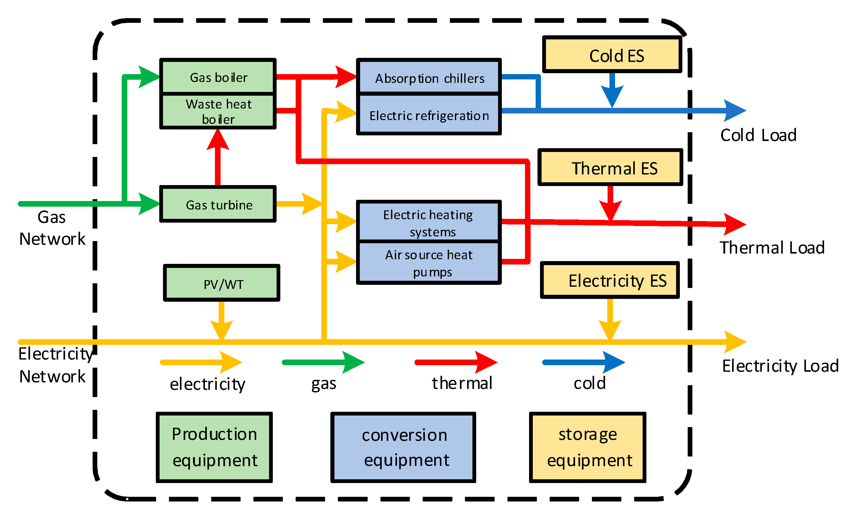
Incentivized IDR differs from incentivized DR in several ways. The coupling connections between various energy sources must be taken into account in the incentive IDR: (1) To achieve the mutual conversion and synergistic utilization of various energy sources, integrated energy service providers utilize energy coupling equipment, such as combined heat and power (CHP), gas turbines, electric boilers, etc.; (2) customer response strategies to various energy sources when participating in incentive-based IDR are also coupled (for example, customers may increase the hours of use of induction cookers while decreasing the usage of other energy sources). The system architecture diagram is shown in Figure 1.

3. Problem Formulation

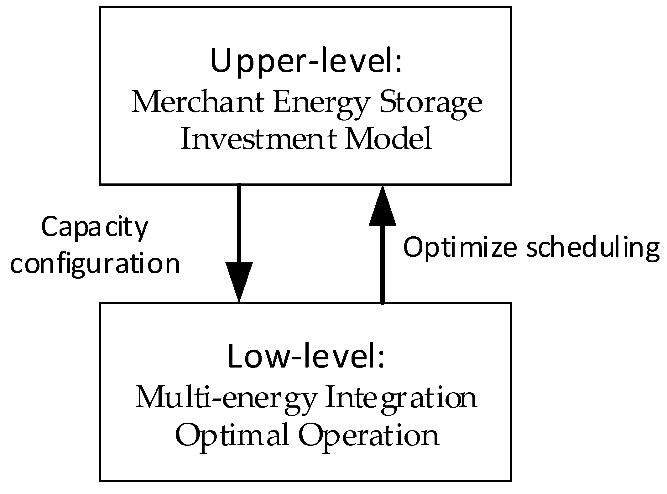
The system’s investment model is explained, and the problem’s multi-energy integration dispatch optimization is then discussed. The specific calculation flow is shown in Figure 2.

The choice is initially made by the higher model, which then transmits to the lower model the values of its decision variables. Based on the upper model, the lower model establishes the feasible domain range, optimizes and derives the optimum value of the objective function, passes the outcome of the lower optimization to the higher model, and iteratively derives the ideal solution and its corresponding optimal value. The outcome of the lower-level optimization is then sent to the upper level, where iteration is used to determine the best solution and its related best value. The best answer to the lower-level issue determines the best answer to the upper-level problem, and the decision variables of the upper-level problem have an impact on the best answer to the lower-level problem. Two-level programming is important because it takes into account the interests of both the upper and lower levels at once, ensuring that the upper level comes first and that the lower level obeys the upper level while still retaining some degree of autonomy within the parameters of the upper level’s decision-making authority.

3.1. The Upper Level: Merchant Investment

3.1.1. Objective Function

The upper-level planning model’s primary goal is to reduce the annualized cost across the investment cycle, which is stated as

$$\min C^U=\min \left[C^{inv,U}+\left(C_{ess}^{buy,U}-C_{ess}^{sell,U}\right)-C^{aux,U}\right]$$

(1)

where $C^{inv,U}$ denotes investment and maintenance costs for energy storage power stations, $C_{ess}^{buy,U}$ denotes the cost of purchasing electricity from the microgrid for energy storage power stations, $C_{ess}^{sell,U}$ denotes the cost of selling electricity to the microgrid by energy storage power stations, and $C^{aux,U}$ denotes energy storage power station service fee.

• Cost of investment and maintenance

$$C^{inv,U}=C_{ess}^{inv}{r}^{CR}+C_{ess}^{main}$$

(2)

$$C_{ess}^{inv}={\displaystyle \sum _{n=1}^{N_{\mathrm{ess}}}\left(c^p{P}_n^{ess,max}+c^e{E}_n^{ess,max}\right)}$$

(3)

$$C_{ess}^{main}={\displaystyle \sum _{t=1}^{T_{life}}{\displaystyle \sum _{n=1}^{N_{main}}{c}_{ess,t,n}^{main}}}$$

(4)

where $C_{ess}^{inv}$ denotes the cost of battery investment; $P_n^{ess,max}$ and $E_n^{ess,max}$ denote the maximum charge/discharge power and the maximum capacity of the energy storage plant at node n; $N_{\mathrm{ess}}$ is the total number of batteries; $c^p$ and $c^e$ are the power cost and capacity cost of the energy storage plant in CNY/kW and CNY/(kWh); $C_{ess}^{main}$ denotes the battery maintenance cost; $c_{ess,t,n}^{main}$ is the daily battery maintenance cost at bus n during interval t; and $T_{life}$ is the battery’s entire life cycle.

$$r^{CR}=\frac{1}{365}\frac{r{\left(1+r\right)}^Y}{{\left(1+r\right)}^Y-1}$$

(5)

where $r^{CR}$ is the discount rate, $r$ is the annual discount rate, and $Y$ is the energy storage life cycle.

2.

Cost of electricity

$$C_{ess}^{buy,U}={\displaystyle \sum }_{d=1}^{N_D}{\displaystyle \sum }_{t=1}^{N_T}{\displaystyle \sum }_{i=1}^{N_{MG}}\left({\lambda }_t^{buy}{P}_{i,t,d}^{buy,ess}\right)$$

(6)

where $N_{MG}$ is the number of microgrids; $N_T$ is the number of dispatch periods; $N_D$ is the number of days; ${\lambda }_t^{buy}$ is the price of electricity bought from the microgrid to the storage plant at time t in CNY/(kWh); and $P_{i,t,d}^{buy,ess}$ is the electricity price of purchasing electricity by energy storage power stations in time slot t of each typical day d.

$$C_{ess}^{sell,U}={\displaystyle \sum }_{d=1}^{N_D}{\displaystyle \sum }_{t=1}^{N_T}{\displaystyle \sum }_{i=1}^{N_{MG}}\left({\lambda }_t^{sell}{P}_{i,t,d}^{sell,ess}\right)$$

(7)

where ${\lambda }_t^{sell}$ is the price of electricity sold to the microgrid from the storage plant at the time t in CNY/(kWh) and $P_{i,t,d}^{sell,ess}$ is the power sold by the storage plant to the microgrid I in time slot t of each typical day d.

3.

The service fee charged by the energy storage

$$C^{aux,U}={\displaystyle \sum }_{d=1}^{N_D}{\displaystyle \sum }_{t=1}^{N_T}{\displaystyle \sum }_{i=1}^{N_{MG}}\left[{\lambda }_t^{aux}\left(P_{i,t,d}^{buy,ess}-P_{i,t,d}^{sell,ess}\right)\right]$$

(8)

where ${\lambda }_t^{aux}$ is the unit price of the service fee paid by the microgrid to the energy storage plant at time t in CNY/(kWh), and $P_{i,t,d}^{buy,ess}$ and $P_{i,t,d}^{sell,ess}$ are the same as above.

3.1.2. Constraints

• Energy storage investment constraints

The ratio between the energy storage plant capacity and the rated power is proportional to the following:

$$p_n^{ess,\max }\cdot \chi =E_n^{ess,\max }$$

(9)

$$C_{ess}^{inv}={\displaystyle \sum _{n=1}^N\left(c^p{P}_n^{ess,max}+c^e{E}_n^{ess,max}\right)}\cdot r^{CR}\le I{C}^{\max ,U}$$

(10)

$$C^{income,U}=\left(C_{ess}^{sell,U}-C_{ess}^{buy,U}\right)+C^{aux,U}\ge {\alpha }^U{C}^{inv,U}$$

(11)

where $\chi$ is the energy multiplier of the energy storage plant; $E_n^{ess,max}$ and $P_n^{ess,max}$ are as described above; $I{C}^{max,U}$ denotes investment constraint; $C^{income,U}$ and $C^{inv,U}$ denote investment income and total investments; and ${\alpha }^U$ indicates the rate of return on investment to ensure revenue.

2.

Energy storage constraints

Consider the battery charge state model represented as follows:

$$E_{i,t+1}^{bat}=E_{i,t}^{bat}+{\eta }_i^{ch}{P}_{i,t}^{ch}-P_{i,t}^{dis}/{\eta }_i^{dis}$$

(12)

$$E_i^{\min }\le E_{i,t}^{bat}\le E_i^{\max }$$

(13)

where $E_{i,t}^{bat}$ denotes the battery i energy during time t, ${\eta }_i^{ch}$ and ${\eta }_i^{dis}$ denote the battery i charge and discharge efficiency, $P_{i,t}^{ch}$ and $P_{i,t}^{dis}$ denote the battery i charge and discharge power during time slot t, and $E_i^{min}$d $E_i^{max}$ note the lower and upper charge state constraints of battery i in terms of preventing the battery from deep discharge and overshoot.

The charging and discharging power constraints are as follows:

$$0\le P_{i,t}^{ch}\le P_i^{ch,\max }$$

(14)

$$0\le P_{i,t}^{dis}\le P_i^{dis,\max }$$

(15)

where $P_{i,t}^{ch}$ and $P_{i,t}^{dis}$ denote battery i charge and discharge power during time t, and $P_i^{ch,max}$ and $P_i^{dis,max}$ denote battery i maximum charge and discharge power.

3.2. The Low Level: Optimal Operation of Multi-Energy Integration

The decision variables for the lower model are the following: power generated by the gas turbine; the absorption chillers; the electric chillers; the electric power consumption; the gas boilers; the heat production power from the heat exchanger; the heat production power from the electricity grid; the power purchased from the energy storage plant by the microgrid; the power purchase stat; the power purchased from the grid; the power and status of the power purchased from storage plants by the microgrid; the power and status of the power sold by the microgrid to storage plants; the power output of an electric chiller; the power consumption of an electric chiller; the power output of a gas boiler; the power output of a heat exchanger; and the power of a heat-making device.

3.2.1. Objective Function

The lower-level target function is both the lowest annual operating cost of the cogeneration-type multi-microgrid system and the lowest annual operating cost of the service-based cooling and heating of the energy storage power plant [34].

$$\min C^L=\min \left[C^{grid,L}+C^{gas,L}+\left(C_{ess}^{sell,L}-C_{ess}^{buy,L}\right)+C^{aux,L}\right]$$

(16)

where $C^{grid,L}$ is the cost of purchased electricity from the grid; $C^{gas,L}$ is the clean fuels cost of gas turbines and gas boilers per typical day; $C_{ess}^{sell,L}$, $C_{ess}^{buy,L}$, and $C^{aux,L}$ are described as above; and L denotes the low level.

• The cost of purchasing electricity from the grid

$$C^{grid,L}={\displaystyle \sum }_{d=1}^{N_D}{\displaystyle \sum }_{t=1}^{N_T}{\displaystyle \sum }_{i=1}^{N_{MG}}\left({\lambda }_t^{buy}{p}_{i,t,d}^{buy}\right)$$

(17)

where ${\lambda }_t^{buy}$ is the purchased electricity price at time t, and $P_{i,t,d}^{buy}$ is the purchased electricity from the grid for the microgrid at time t on each typical day d.

2.

The cost of a gas turbine

$$C^{gas,L}=c^{gas}{\displaystyle \sum }_{d=1}^{N_D}{\displaystyle \sum }_{t=1}^{N_T}{\displaystyle \sum }_{i=1}^{N_{MG}}\left(p_{i,t,d}^{GT}/{\eta }^{\mathrm{GT}}{\eta }^{\mathrm{NG}}+q_{i,t,d}^{\mathrm{GB}}/{\eta }^{\mathrm{GB}}{\eta }^{\mathrm{NG}}\right)$$

(18)

where $c^{gas}$ is the price of clean fuel in CNY/kg; $p_{i,t,d}^{GT}$ is the output power of the gas turbine at time t for the microgrid i on each typical day d; ${\eta }^{GT}$ is the power generation efficiency of the microturbine; ${\eta }^{NG}$ is the thermal value of the clean fuel, which is 143 kJ/g; $q_{i,t,d}^{GB}$ is the output thermal power of the gas turbine at time t of the microgrid i on each typical day d; and ${\eta }^{GB}$ is the efficiency of the gas boiler.

3.2.2. Constraints

The optimal lower-level operation combined a cooling, heating, and power multi-microgrid system. The equation constraints to be satisfied are the cold power balance constraint, the thermal power balance constraint, the electric power balance constraint, and the waste heat boiler waste heat balance constraint. The inequalities constraints to be satisfied are the microgrid equipment output constraint, microgrid power purchase from the grid constraint, and microgrid and storage power plant power balance constraints. Additionally, the constraints for each typical day are as follows:

• Power balance constraint

$$\left(p_{i,t,d}^{\mathrm{GT}}+p_{i,t,d}^{\mathrm{WT}}+p_{i,t,d}^{\mathrm{PV}}\right)+\left(p_{i,t,d}^{buy,ess}-p_{i,t,d}^{sell,ess}\right)+p_{i,t,d}^{\mathrm{grid}}=p_{i,t,d}^{\mathrm{load}}+\left(p_{i,t,d}^{\mathrm{EC}}+p_{i,t,d}^{\mathrm{EH}}\right)$$

(19)

where $p_{i,t,d}^{grid}$ indicates electrical power purchased from the grid; $p_{i,t,d}^{GT}$ is the gas turbine output power generated by microgrid i at time t on each typical day; $P_{i,t,d}^{WT}$ is the wind power generated by microgrid i at time t on each typical day; $P_{i,t,d}^{PV}$ is the photovoltaic power generated by microgrid i at time t on each typical day; $P_{i,t,d}^{EC}$ is the power of electric cooling consumed by microgrid i at time t on each typical day; $P_{i,t,d}^{EH}$ is the power of electric heating consumed by microgrid i at time t on each typical day; $P_{i,t,d}^{load}$ is the electric power consumed by microgrid i at time t on each typical day microgrid electric load power.

$${\displaystyle \sum }_{i=1}^N\left(p_{i,t,d}^{buy,ess}-p_{i,t,d}^{sell,ess}\right)=p_{t,d}^{dis,ess}-p_{t,d}^{ch,ess}$$

(20)

The left side of the equation is the sum of the purchased and sold electric power of each CCHP microgrid and energy storage power station, and the right side of the equation is the charging and discharging power of the energy storage power station.

2.

Cooling load of CCHP constraint

$$q_{i,t,d}^{\mathrm{AC}}+q_{i,t,d}^{EC}=q_{i,t,d}^{\mathrm{cool}}$$

(21)

$$q_{i,t,d}^{EC}={\eta }^{\mathrm{EC}}{p}_{i,t,d}^{\mathrm{EC}}$$

(22)

where $q_{i,t,d}^{AC}$is the cold load of the absorption chiller of the aggregate area i at time t on each typical day d; $q_{i,t,d}^{EC}$ indicates the cold load of electric cooling; $q_{i,t,d}^{cool}$is the cold load power of the aggregate area i at time t on each typical day; ${\eta }^{EC}$is the energy efficiency ratio of the electric chiller; and $P_{i,t,d}^{EC}$is the electrical power of refrigeration.

3.

Heating load of CCHP constraint

$$q_{i,t,d}^{\mathrm{GHB}}+q_{i,t,d}^{HEX}+q_{i,t,d}^{EH}=q_{i,t,d}^{\mathrm{heat}}$$

(23)

$$q_{i,t,d}^{EH}={\eta }^{\mathrm{EH}}{p}_{i,t,d}^{\mathrm{EH}}$$

(24)

where $q_{i,t,d}^{GHB}$ is the heat power of the gas boiler of the aggregate area i at time t on each typical day d; $q_{i,t,d}^{HEX}$ is the heating power of the heat exchanger of the aggregate area i at time t of each typical day; $q_{i,t,d}^{EH}$ indicates the heating power of electric heating; $q_{i,t,d}^{heat}$ is the thermal load power of the aggregate area i at time t of each typical day; and ${\eta }^{EH}$ is the energy efficiency ratio of electric heating.

4.

The waste heat load of the CCHP constraint

$$q_{i,t,d}^{\mathrm{AC}}/{\eta }^{\mathrm{AC}}+q_{i,t,d}^{\mathrm{HEX}}/{\eta }^{\mathrm{HX}}={\eta }^{\mathrm{WH}}{\gamma }^{\mathrm{GT}}{p}_{i,t,d}^{\mathrm{GT}}$$

(25)

where ${\eta }^{WH}$ is the efficiency of the waste heat boiler; ${\gamma }^{GT}$ is the thermoelectric ratio of the gas turbine; ${\eta }^{AC}$ is the energy efficiency ratio of the absorption chiller; and ${\eta }^{HX}$is the efficiency of the heat exchanger.

5.

CCHP output constraint

$$p^{GT,\min }\le p_{i,t,d}^{\mathrm{GT}}\le p^{GT,\max },q^{HEX,\min }\le q_{i,t,d}^{\mathrm{HEX}}\le q^{HEX,\max }$$

(26)

$$q^{AC,\min }\le q_{i,t,d}^{AC}\le q^{AC,\max },p^{EC,\min }\le p_{i,t,d}^{EC}\le p^{EC,\max }$$

(27)

$$q^{GHB,\min }\le q_{i,t,d}^{GHB}\le q^{GHB,\max },p^{EH,\min }\le p_{i,t,d}^{EH}\le p^{EH,\max }$$

(28)

where $p^{GT,min}$ and $p^{GT,max}$ are the minimum and maximum output power values of the gas turbine; $q^{HEX,min}$ and $q^{HEX,max}$ are the minimum and maximum values of the output power of heat exchange; $q^{AC,min}$ and $q^{AC,max}$ are the minimum and maximum output power values of the absorption chillers; $p^{EC,min}$ and $p^{EC,max}$ are the minimum and maximum output power values of the electric chillers; $q^{GHB,min}$ and $q^{GHB,max}$ are the minimum and maximum output power values of the gas boilers; and $p^{EH,min}$ and $p^{EH,max}$ are the minimum and maximum output power values of the electric heating.

6.

Power output constraint

$$0\le p_{i,t,d}^{\mathrm{grid}}\le p^{\mathrm{g}2\mathrm{mg},\max }$$

(29)

$$0\le p_{i,t,d}^{sell,ess}\le p^{ess,mg,\max }$$

(30)

$$0\le p_{i,t,d}^{buy,ess}\le p^{ess,mg,\max }$$

(31)

where $p^{g2mg,max}$ is the maximum power purchased from the grid by the microgrid, and $p^{ess,mg,max}$ is the maximum interaction power between the microgrid and storage plant.

4. Solution Methodology

4.1. Reformulation

The lower model’s Lagrangian function was initially built. The lower model can be transformed into the upper model with the additional constraints and the transformed single-layer model, where the optimization goals and constraints of the original upper-layer model are present according to the constructed Lagrangian function and the KKT complementary relaxation condition.

$$\min f(x)$$

(32)

$$\left\{\begin{array}{l}{h}_i(x)=0,i=1,2,3\cdots m\\ g_j(x)\le 0,j=1,2,3\cdots n\end{array}\right.$$

(33)

The Lagrangian function of the low-level model for the original problem was defined as follows:

$$L(x,\alpha ,\beta )=f(x)+{\displaystyle \sum _{i=1}^m{\alpha }_i{h}_i(x)}+{\displaystyle \sum _{j=1}^n{\beta }_i{g}_j(x)}$$

(34)

Additionally, the Lagrangian function of the low-level model can be reformulated as

$$\begin{array}{l}L=\left(C^{grid,L}+C^{gas,L}+\left(C_{ess}^{sell,L}-C_{ess}^{buy,L}\right)-C^{aux,L}\right)\\ +{\alpha }_1\left[\left(p_{i,t,d}^{\mathrm{GT}}+p_{i,t,d}^{\mathrm{WT}}+p_{i,t,d}^{\mathrm{PV}}\right)+p_{i,t,d}^{\mathrm{grid}}+\left(p_{i,t,d}^{buy,ess}-p_{i,t,d}^{sell,ess}\right)-p_{i,t,d}^{\mathrm{load}}-\left(p_{i,t,d}^{\mathrm{EC}}+p_{i,t,d}^{\mathrm{EH}}\right)\right]\\ +{\alpha }_2\left[{\displaystyle {\displaystyle \sum }_{i=1}^N}\left(p_{i,t,d}^{buy,ess}-p_{i,t,d}^{sell,ess}\right)-\left(p_{t,d}^{dis,ess}-p_{t,d}^{ch,ess}\right)\right]\\ +{\alpha }_3\left[q_{i,t,d}^{\mathrm{AC}}+q_{i,t,d}^{EC}-q_{i,t,d}^{\mathrm{cool}}\right]+{\alpha }_4\left[q_{i,t,d}^{\mathrm{GHB}}+q_{i,t,d}^{HEX}+q_{i,t,d}^{EH}-q_{i,t,d}^{\mathrm{heat}}\right]\\ +{\alpha }_5\left[q_{i,t,d}^{\mathrm{AC}}/{\eta }^{\mathrm{AC}}+q_{i,t,d}^{\mathrm{HEX}}/{\eta }^{\mathrm{HX}}-{\eta }^{\mathrm{WH}}{\gamma }^{\mathrm{GT}}{p}_{i,t,d}^{\mathrm{GT}}\right]\\ +{\beta }_1\left[p^{GT,\min }-p_{i,t,d}^{\mathrm{GT}}\right]+{\beta }_2\left[p_{i,t,d}^{\mathrm{GT}}-p^{GT,\max }\right]\\ +{\beta }_3\left[q^{HEX,\min }-q_{i,t,d}^{\mathrm{HEX}}\right]+{\beta }_4\left[q_{i,t,d}^{\mathrm{HEX}}-q^{HEX,\max }\right]\\ +{\beta }_5\left[q^{AC,\min }-q_{i,t,d}^{AC}\right]+{\beta }_6\left[q_{i,t,d}^{AC}-q^{AC,\max }\right]\\ +{\beta }_7\left[p^{EC,\min }-p_{i,t,d}^{EC}\right]+{\beta }_8\left[p_{i,t,d}^{EC}-p^{EC,\max }\right]\\ +{\beta }_9\left[q^{GHB,\min }-q_{i,t,d}^{GHB}\right]+{\beta }_{10}\left[q_{i,t,d}^{GHB}-q^{GHB,\max }\right]\\ +{\beta }_{11}\left[p^{EH,\min }-p_{i,t,d}^{EH}\right]+{\beta }_{12}\left[p_{i,t,d}^{EH}-p^{EH,\max }\right]\\ +{\beta }_{13}\left[-p_{i,t,d}^{\mathrm{grid}}\right]+{\beta }_{14}\left[p_{i,t,d}^{\mathrm{grid}}-p^{\mathrm{g2mg,max}}\right]\\ +{\beta }_{15}\left[-p_{i,t,d}^{sell,ess}\right]+{\beta }_{16}\left[p_{i,t,d}^{sell,ess}-p^{ess,mg,\max }\right]\\ +{\beta }_{17}\left[-p_{i,t,d}^{buy,ess}\right]+{\beta }_{18}\left[p_{i,t,d}^{buy,ess}-p^{ess,mg,\max }\right]\end{array}$$

(35)

where the first row indicates the objective function, the second to fifth rows indicate the equation constraint, and the sixth to fourteenth rows indicate the inequality constraint.

If the dual gap is 0 (strong dual) and the Lagrangian function is differentiable to x, the best solution to the original issue and the dual problem may be found.

$$\left\{\begin{array}{l}{\nabla }_{x}L(x,\alpha ,\beta )=0\\ {\beta }_j{g}_j(x)=0,j=1,2,3\cdots n\\ h_i(x)=0,i=1,2,3\cdots m\\ g_j(x)\le 0,j=1,2,3\cdots n\\ {\beta }_j\ge 0,j=1,2,3\cdots n\end{array}\right.$$

(36)

The viable solution must satisfy the KKT requirement. The Lagrangian is differentiable if x is the best solution to the original problem and the differentiation at x is equal to 0. According to the primary feasibility criteria, the ideal solution to the original issue must satisfy all of its restrictions. The dual feasibility criterion states that the dual problem’s constraints must be satisfied by the dual problem’s optimum solution.

The derivatives of each variable x were determined as follows:

$$A_1^{gt}+{\alpha }_1-A_2^{gt}{\alpha }_5-{\beta }_1+{\beta }_2=0$$

(37)

$${\alpha }_4+A_1^{hex}{\alpha }_5-{\beta }_3+{\beta }_4=0$$

(38)

$${\alpha }_3-A_1^{ac}{\alpha }_5-{\beta }_5+{\beta }_6=0$$

(39)

$$-{\alpha }_1+{\alpha }_3-{\beta }_7+{\beta }_8=0$$

(40)

$$A_1^{ghb}+{\alpha }_4-{\beta }_9+{\beta }_{10}=0$$

(41)

$$-{\alpha }_1+{\alpha }_4-{\beta }_{11}+{\beta }_{12}=0$$

(42)

$$A_1^{\mathrm{grid}}+{\alpha }_1-{\beta }_{13}+{\beta }_{14}=0$$

(43)

$$A_1^{sell,ess}-{\beta }_{15}+{\beta }_{16}=0$$

(44)

$$A_1^{buy,ess}-{\beta }_{17}+{\beta }_{18}=0$$

(45)

where A denotes the constant term of the derivative of different variables, the superscript denotes the variable, and the subscript denotes the number of constant terms of that variable.

The complementary slackness condition is expressed as follows:

$${\beta }_1\ge 0,p^{GT,\min }-p_{i,t,d}^{\mathrm{GT}}\le 0,{\beta }_1\left(p^{GT,\min }-p_{i,t,d}^{\mathrm{GT}}\right)=0$$

(46)

$${\beta }_2\ge 0,p_{i,t,d}^{\mathrm{GT}}-p^{GT,\max }\le 0,{\beta }_2\left(p_{i,t,d}^{\mathrm{GT}}-p^{GT,\max }\right)=0$$

(47)

$${\beta }_3\ge 0,q^{HEX,\min }-q_{i,t,d}^{\mathrm{HEX}}\le 0,{\beta }_3\left(q^{HEX,\min }-q_{i,t,d}^{\mathrm{HEX}}\right)=0$$

(48)

$${\beta }_4\ge 0,q_{i,t,d}^{\mathrm{HEX}}-q^{HEX,\max }\le 0,{\beta }_4\left(q_{i,t,d}^{\mathrm{HEX}}-q^{HEX,\max }\right)=0$$

(49)

$${\beta }_5\ge 0,q^{AC,\min }-q_{i,t,d}^{AC}\le 0,{\beta }_5\left(q^{AC,\min }-q_{i,t,d}^{AC}\right)=0$$

(50)

$${\beta }_6\ge 0,q_{i,t,d}^{AC}-q^{AC,\max }\le 0,{\beta }_6\left(q_{i,t,d}^{AC}-q^{AC,\max }\right)=0$$

(51)

$${\beta }_7\ge 0,p^{EC,\min }-p_{i,t,d}^{EC}\le 0,{\beta }_7\left(p^{EC,\min }-p_{i,t,d}^{EC}\right)=0$$

(52)

$${\beta }_8\ge 0,p_{i,t,d}^{EC}-p^{EC,\max }\le 0,{\beta }_8\left(p_{i,t,d}^{EC}-p^{EC,\max }\right)=0$$

(53)

$${\beta }_9\ge 0,q^{GHB,\min }-q_{i,t,d}^{GHB}\le 0,{\beta }_9\left(q^{GHB,\min }-q_{i,t,d}^{GHB}\right)=0$$

(54)

$${\beta }_{10}\ge 0,q_{i,t,d}^{GHB}-q^{GHB,\max }\le 0,{\beta }_{10}\left(q_{i,t,d}^{GHB}-q^{GHB,\max }\right)=0$$

(55)

$${\beta }_{11}\ge 0,p^{EH,\min }-p_{i,t,d}^{EH}\le 0,{\beta }_{11}\left(p^{EH,\min }-p_{i,t,d}^{EH}\right)=0$$

(56)

$${\beta }_{12}\ge 0,p_{i,t,d}^{EH}-p^{EH,\max }\le 0,{\beta }_{12}\left(p_{i,t,d}^{EH}-p^{EH,\max }\right)=0$$

(57)

$${\beta }_{13}\ge 0,-p_{i,t,d}^{\mathrm{grid}}\le 0,{\beta }_{13}\left(-p_{i,t,d}^{\mathrm{grid}}\right)=0$$

(58)

$${\beta }_{14}\ge 0,p_{i,t,d}^{\mathrm{grid}}-p^{\mathrm{g}2\mathrm{mg},\max }\le 0,{\beta }_{14}\left(p_{i,t,d}^{\mathrm{grid}}-p^{\mathrm{g}2\mathrm{mg},\max }\right)=0$$

(59)

$${\beta }_{15}\ge 0,-p_{i,t,d}^{sell,ess}\le 0,{\beta }_{15}\left(-p_{i,t,d}^{sell,ess}\right)=0$$

(60)

$${\beta }_{16}\ge 0,p_{i,t,d}^{sell,ess}-p^{ess,mg,\max }\le 0,{\beta }_{16}\left(p_{i,t,d}^{sell,ess}-p^{ess,mg,\max }\right)=0$$

(61)

$${\beta }_{17}\ge 0,-p_{i,t,d}^{buy,ess}\le 0,{\beta }_{17}\left(-p_{i,t,d}^{buy,ess}\right)=0$$

(62)

$${\beta }_{18}\ge 0,p_{i,t,d}^{buy,ess}-p^{ess,mg,\max }\le 0,{\beta }_{18}\left(p_{i,t,d}^{buy,ess}-p^{ess,mg,\max }\right)=0$$

(63)

Up to this step, the two-level optimization problem is transformed into a single-level problem:

$$\min C^U$$

(64)

s.t. (9)–(15), (37)–(45), (46)–(63)

The preceding models (37)–(45) and (46)–(63) are nonlinear, and the complementing slackness conditions are decoupled and turned into a linear model via the big-M approach as per the following equation:

$$\left\{\begin{array}{l}0\le {\beta }_j\le M{z}_j,\forall j\\ 0\le g_j(x)\le M\left(1-z_j\right),\forall j\\ z_j\in \left\{0,1\right\},\forall j\end{array}\right.$$

(65)

where M is a sizable constant and $z_j$ is a binary variable, and M is frequently chosen based on the variable’s range. To improve the effectiveness of the Big-M technique, it should be at the highest limit to the left.

Up to this step, the original problem is transformed into a single-layer mixed-integer model to solve.

4.2. Algorithm Steps

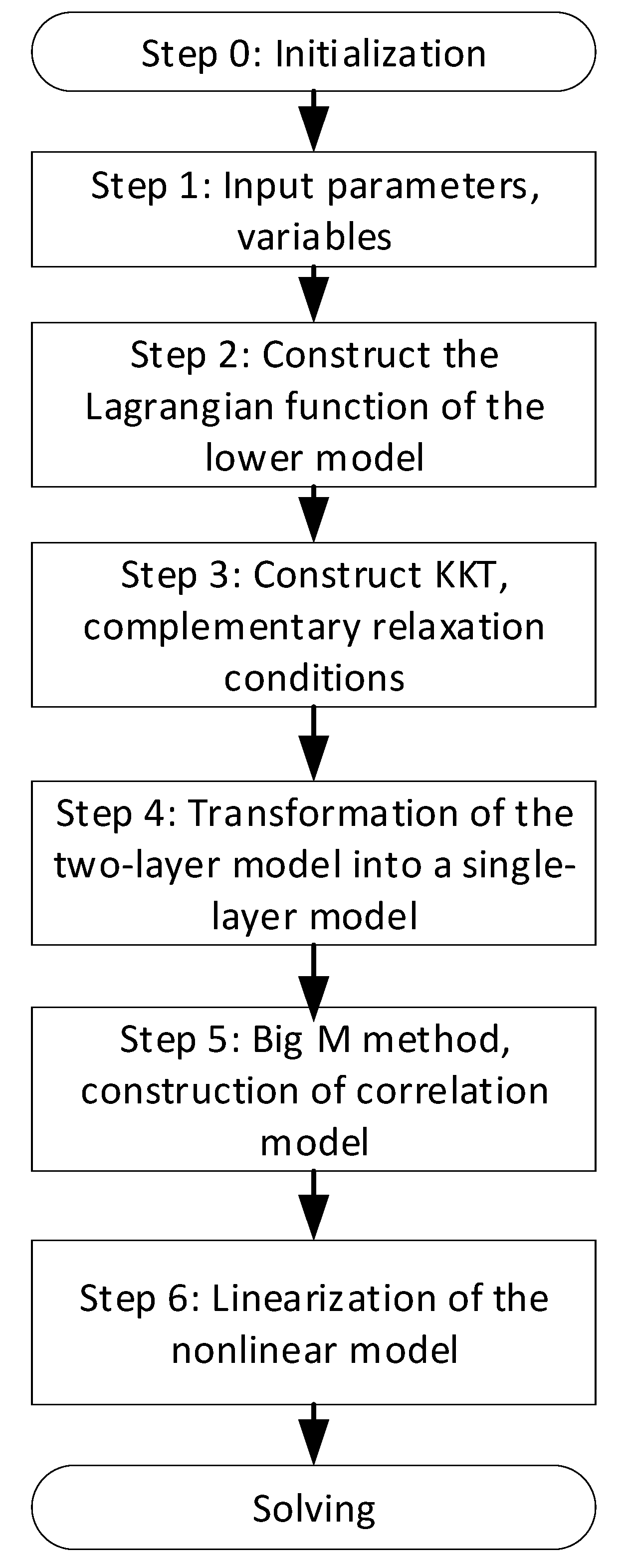
Figure 3 depicts the process of finding a solution. It is challenging to explicitly resolve the coupling connection between the upper-layer and lower-layer models. The converted single-layer nonlinear model is created by building the Lagrangian function of the lower-level model, which is based on the KKT complementary relaxation conditions of the lower model, and by converting the lower model into the upper model restrictions. The converted single-layer nonlinear model is then linearized using the Big-M approach. The procedure for converting the transformed single-layer nonlinear model into a single-level mixed integer linear model is thus detailed. We use the licensed solver Gurobi in Matlab 2017 to resolve the mixed-integer linear programming issue.

5. Results and Discussion

5.1. Experimental Settings

The CCHP multi-microgrid system used in the example consists of two CCHP microgrids: MG1 represents a residential community, with smaller heating and cooling loads, and smaller new energy installations; MG2 represents an industrial community with a large cooling, heating, and electricity load, as well as a large installed capacity of new energy; and each microgrid user is directly connected to a shared energy storage plant (other parameters can be found in [34]). The natural gas price is 3 CNY/m³, the power purchase tariff of the grid adopts the timeshare tariff, and the time-of-use (TOU) price between the microgrid and the storage power plant is shown in

Table 1. Time-of-use price.

	Time	Electricity Price (CNY/kW·h)
		Buy from Grid	Buy from ES	Sell to ES
Peak	08:00–12:00	1.35	1.15	0.90
	17:00–21:00
Flat	12:00–17:00	0.80	0.75	0.55
	21:00–24:00
valley	00:00–08:00	0.35	0.40	0.20

. The unit price of the service fee paid by the microgrid for the energy storage plant is 0.05 CNY/(kW·h), the charging and discharging efficiency of the energy storage plant is 0.9, the operating range of stored energy is 20~80%, and the initial stored energy is 20%. The capacity cost of the energy storage plant refers to the average winning price of 1248 CNY/(kW·h) for a lithium iron phosphate battery in an energy storage project, the power cost of 980 CNY/kW, the operation and maintenance cost 60 CNY/(year/kW), the life cycle of the energy storage plant is 8 years, and the annual discount rate is 0.1. To simplify the calculation, a typical year of 365 days is used to calculate the investment return for one year.

The following example situation is used: a multi-microgrid system of the cold-heat-electricity cogeneration type uses the energy storage power plant’s charging and discharging services.

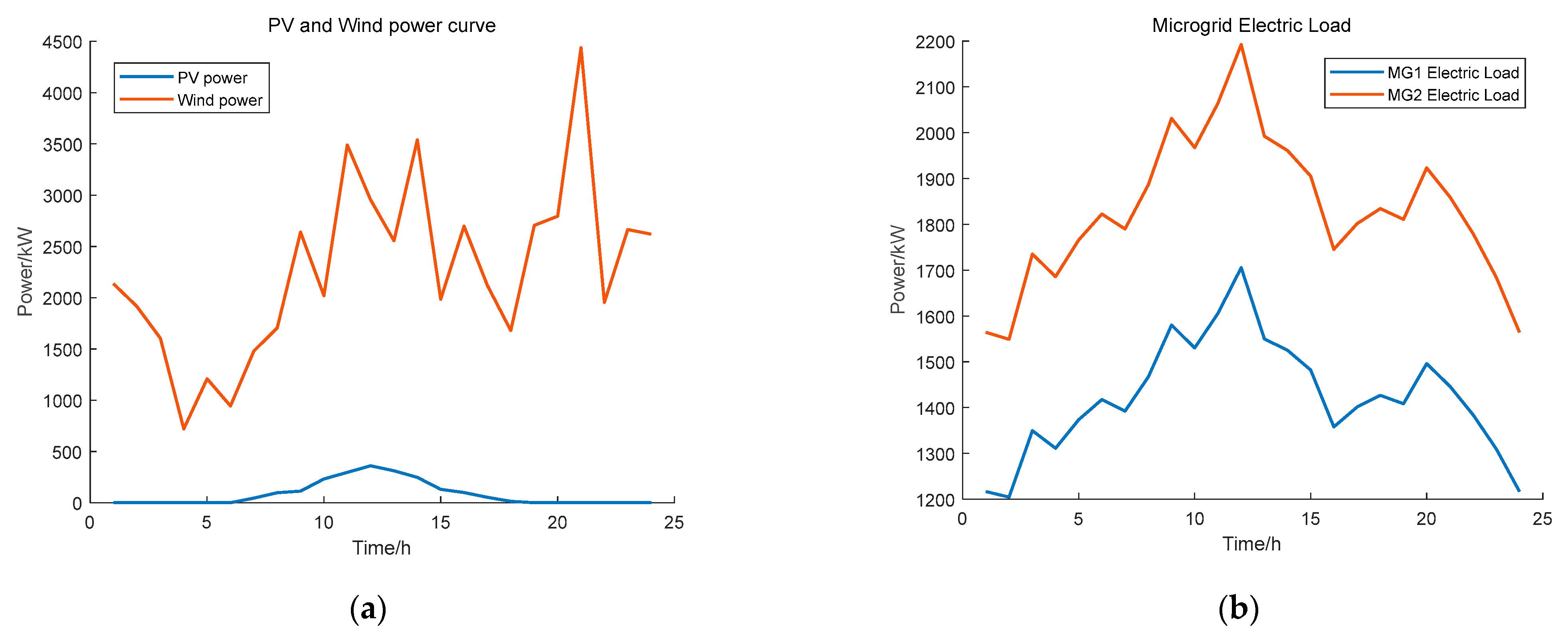
In Figure 4a, the red curve indicates the wind power output, and the blue curve indicates the PV output. In Figure 4b, the blue curve indicates the electric load of Microgrid 1, and the red curve indicates the electric load of Microgrid 2. In this paper, we study the investment returns of the clustered power plants in multiple microgrids with different load characteristics, such that their climatic characteristics are generally kept consistent and the local renewable resource profile is expressed in terms of uniform PV and wind power. Additionally, one of the themes of this paper is represented in Figure 4b. In order to represent multiple microgrids with different load characteristics, one energy storage plant is responsible for the operation of multiple microgrids.

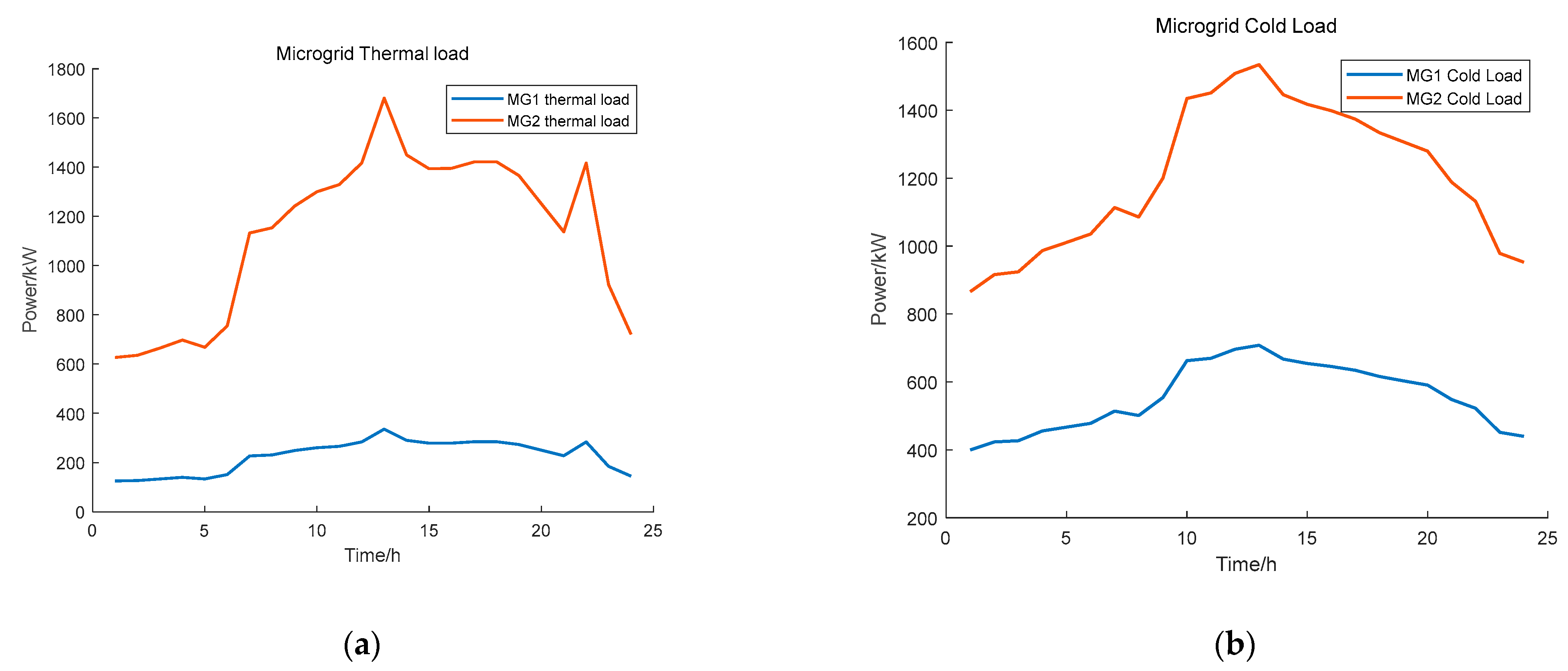
In Figure 5a, the blue line indicates the heat load curve of Microgrid 1, and the red line indicates the heat load curve of Microgrid 2. In Figure 5b, the blue line indicates the cold load curve of Microgrid 1, and the red line indicates the cold load curve of Microgrid 2. Figure 5 serves the same purpose as Figure 4b. This is performed in order to illustrate the different thermal load characteristics and cold load characteristics between the multiple microgrids. This allows a comprehensive representation of the cold and thermal load characteristics of multiple microgrids.

5.2. Energy Storage Configuration Analysis

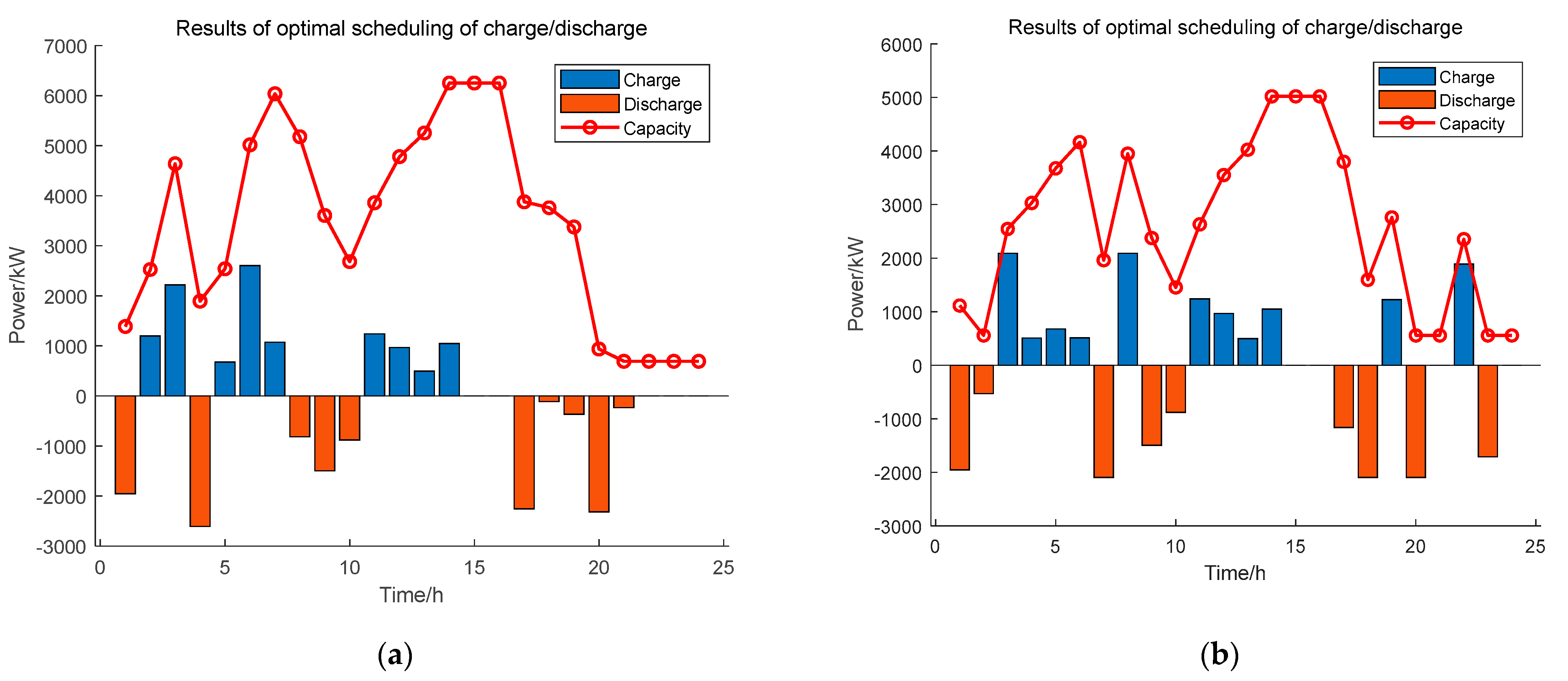
The investment and maintenance costs of the electric energy storage device are evenly shared according to the life cycle and are included in the annual operating cost of the combined cooling, heating, and power multi-microgrid system. The storage power plant service was launched, and a multi-microgrid system with complimentary cold and hot power was present. Figure 6 displays the optimization results for the storage power plant’s charging and discharging behavior on a typical day. If the storage power plant is positive, the blue bar indicates that it is charging; if it is negative, the red bar indicates that it is discharging. The energy storage power plant’s charging status is represented by the red curve.

In the microgrid represented by residential and commercial communities, electric heating is the most common heating equipment. Therefore, in this paper, two scenarios were analyzed from the actual situation of investors in order to advance closer to the real scenario and to determine whether the community is equipped with electric heating equipment or not. The night is the peak period of heat load; the community that is without electric heating (Figure 6a) has their night energy storage capacity gradually and evidently reduced, while the community with electric heating (Figure 6b) had several back charging processes, which have a clear relationship with the charging and discharging tariff. Thus, it can be seen that the existing value of energy storage power plant is of a low price for charging. In addition, the discharge in the peak period is for producing the electricity price difference revenue, which further confirms the revenue principle of the energy storage power plant. In the following section, the specific benefits will be analyzed from the perspective of a quantitative relationship.

In addition, we compared and analyzed the centralized different schemes, as shown in

Table 2. Scheduling results for the different scenarios.

	ES Capacity	Max Power	Revenue	Investment	Maintenance	Payback
Scheme 1	6946.4	2605.7	445	1122.3	15.6	2.6
Scheme 2	5579.9	2093.1	470	901.5	12.6	2.0

: Scheme 1 indicates three microgrids, but does not include electric heating modeling; Scheme 2 indicates three microgrids and includes electric heating modeling. The ES capacity denotes optimal capacity, the unit is kWh; Max power denotes maximum charging and discharging power in kW; Revenue is the annual return on investment in CNY 10,000; the total investment cost is Investment in CNY 10,000; Maintenance denotes the annual maintenance cost in CNY 10,000; and Payback is investment payback year.

From the calculation results, the outcomes of Scheme 1’s design for energy storage and charging/discharging power are higher than those of Scheme 2, while the benefit is less than Scheme 2; compared to Scheme 2 (which uses electric heating), Scheme 1 (which is without electric heating) has higher investment and annual maintenance costs, as well as a longer payback period. From the results of this experiment, the following conclusions can be drawn: when investors build energy storage power plants, they should make specific analyses according to the community situation and should not increasingly invest, but instead make reasonable quantitative calculations according to the actual equipment in the community. As shown in this case, the scheme involving the design of the energy storage power plant being calculated according to the electric heating equipment is significantly better.

5.3. Configuration Results under Different Time-of-Use (TOU)

The calculated allocation results and payback cycle results for the same multi-energy scenario, which was based on the incentive tariffs of a different strategy, are shown in

Table 3. Investment results under different TOU prices.

	ES Capacity	Max Power	Revenue	Investment	Maintenance	Payback
TOU 1	6946.4	2605.7	445.0	1122.3	15.6	2.6
TOU 2	4460.1	1673.1	327.2	720.6	10.0	2.3
TOU 3	5201.2	1951.1	481.4	840.3	11.7	1.8

. Option 2 is based on Option 1 with all prices reduced, and Option 3 is based on Option 1 with all prices increased.

This part employs three demand response incentive tariff techniques to examine the effects of various tariff systems on the investment advantages of energy storage facilities and to make suggestions for the industry’s future. The tariff is not strictly correct, but only examines the impact of different price trends on energy storage configurations. It can be seen through Option 2 and Option 3 that the higher the purchase and sale price of electricity, the higher the return; the lower the purchase and sale price of electricity, the lower the return; however, the investment payback period is less than Option 1, and the storage battery capacity is smaller than Option 1.

Electricity price 1 is the middle price, electricity price 2 is the low price, and electricity price 3 is the high price. There are several interesting conclusions to be made in the middle of this: (1) Tariff 3 is the highest, but the storage capacity and charging/discharging capacity of the power plant are lower than the storage capacity and charging/discharging power of the middle tariff. While Tariff 3 has the highest return, which shows that the high and low returns do not correspond to the storage capacity and maximum charging/discharging power, there is still a need to design the scheme according to the actual situation. (2) Accordingly, the investment of Option 3 is lower than Option 1 regarding the tariff. Moreover, the maintenance cost is much lower, and the payback years are also much lower. (3) From the physical energy storage capacity, as well as the charging and discharging power from the economic investment cost, maintenance cost, and payback years, two major aspects of several small indicators verify that the design of an energy storage power plant needs to be quantified and analyzed according to the actual situation.

The different tariffs are shown in

Table 4. Different TOU prices.

	Time	TOU 1			TOU 2			TOU 3
		Grid	ES_Sell	ES_Buy	Grid	ES_Sell	ES_Buy	Grid	ES_Sell	ES_Buy
Peak	08:00–12:00	1.35	1.15	0.90	1.15	1.00	0.85	1.50	1.20	0.95
	17:00–21:00
Flat	12:00–17:00	0.80	0.75	0.55	0.75	0.70	0.50	0.90	0.85	0.65
	21:00–24:00
valley	00:00–08:00	0.35	0.40	0.20	0.3	0.35	0.15	0.40	0.50	0.30

.

There is still a great deal of work to be completed on other tariff combination choices, which will be evaluated alongside the electricity spot market.

5.4. MG Power Purchase and Sale Results

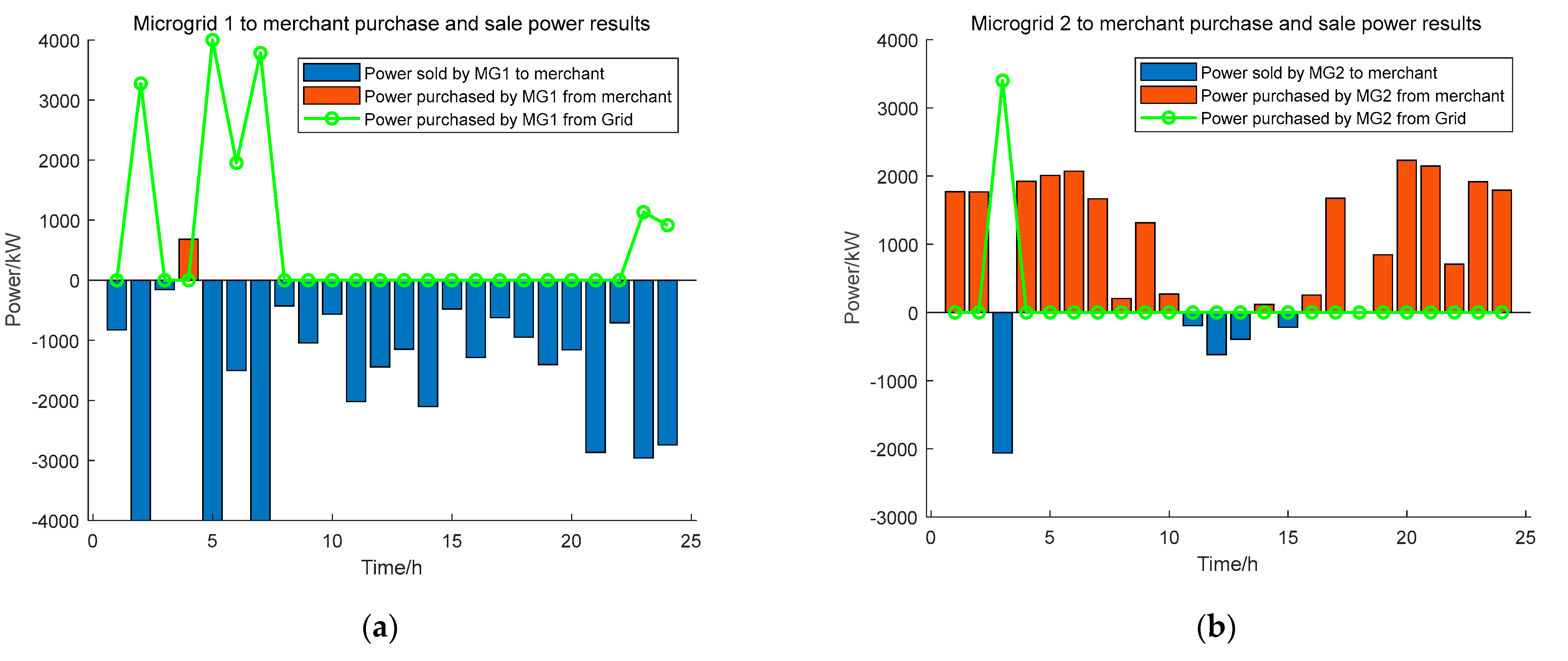
We examine the scheduling outcomes for a typical day and compare the performance of two typical microgrids: one has an energy-rich, power-output-dominated structure, while the other is an energy-deficient, power-input-dominated one. The power purchase and sale of Microgrid 1 is shown in Figure 7a, and the power purchase and sale of Microgrid 2 is shown in Figure 7b. The microgrid receives electricity from the energy storage plant, as indicated by the red bar, and sells power to the energy storage plant, as indicated by the blue bar. The green curve indicates the power purchased by the microgrid from the grid.

In Figure 7a, Microgrid 1 (energy-rich, power-output-dominated structure) buys 682.9 kW from the storage plant between the hours of 3:00–4:00, while selling electricity to the storage plant during the remaining hours. Since Microgrid 1 simulates an energy-rich power-output-dominated structure community, the dispatching results are consistent with the simulated scenario. In Figure 7b, Microgrid 2 (energy-deficient, power-input-dominated structure) sells 2062.6 kW, 196 kW, 620 kW, 394.7 kW, and 218.1 kW to the storage power plant three times between the hours of 2:00–3:00, 10:00–11:00, 11:00–12:00, 12:00–13:00, and 14:00–15:00, respectively; during the other periods, Microgrid 2 purchases electricity from the storage power plant. The scheduling outcomes are accurate given that Microgrid 2 mimics a residential neighborhood.

5.5. MG Scheduling Results

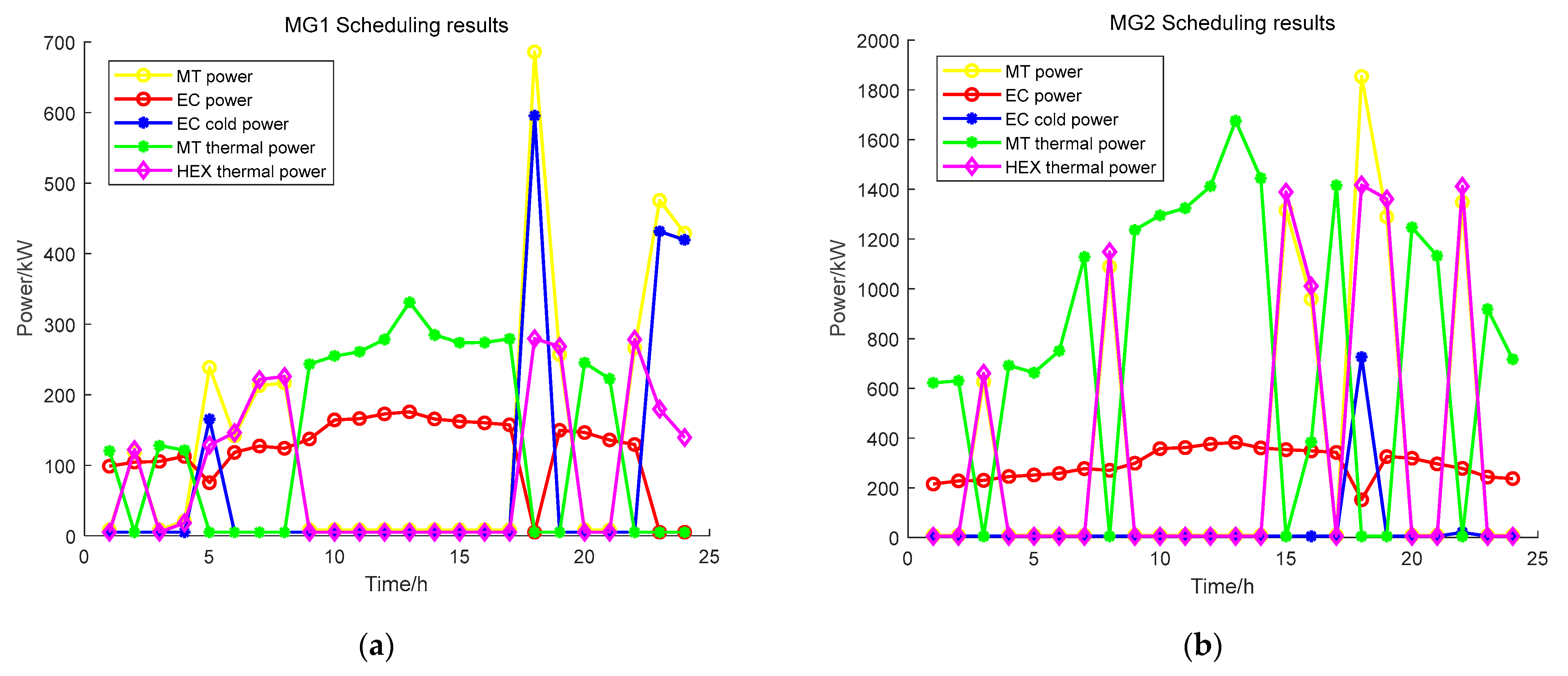
The multiple energy outputs of Microgrid 1 are shown in Figure 8a, and the multiple energy outputs of Microgrid 2 are shown in Figure 8b. The yellow curve represents the gas turbine output, the red curve represents the electric power of cooling output, the blue curve represents the electric cooling power output, the green curve represents the gas turbine heating power, and the purple curve represents the waste heat production power.

Microgrid 1 is an energy-rich, power-output-dominated structure, and Microgrid 2 is an energy-deficient, power-input-dominated structure. Gas turbines are primarily used to generate heat, and electric refrigeration is primarily used to generate cold temperatures.

Microgrid 1 is energy-rich and transmits electricity to the outside. The power of gas turbines is similar to that of refrigeration, and the electrical power of gas turbines is used for refrigeration, indicating that the electrical load is adequately supplied by internal renewable energy sources. Microgrid 2 is energy-poor and the use of gas turbines is significantly increased, showing the important role of gas turbines in resource-poor communities. This further validates that communities with different resource characteristics and load characteristics have different electricity-use effectiveness. During the construction of energy storage plants, a quantitative analysis needs to be conducted with full consideration of different community resource endowments. This summary-type experiment mainly examines the impact brought by resource endowment, while the above mainly examines the difference in electricity price, which is a comparative analysis from different perspectives.

6. Conclusions

The main purpose of this study is to address the economics of the most relevant issues for investors from a theoretical perspective. Additionally, a two-stage model of an integrated energy demand response was constructed in this work, and experimental data were used to demonstrate the quantitative link between two of investors’ primary concerns: namely, return on investment and the relationship between the investment cycle and demand response.

• From the perspective of energy storage plants, the return on investment is directly related to the price of electricity. The high price of electricity and its high return does not mean high investment; on the contrary, a small investment is verified from several angles. This means that the investment is small, but that the return is high, which is related to the community having the necessary equipment. Therefore, when building an energy storage power plant, quantitative calculations need to be made based on community-specific equipment;
• The importance of resource endowment, from a community perspective, is closely related to the community’s equipment configuration. In resource-rich areas, the benefits of transmitting electricity outward and matching gas turbines with refrigeration are seen in the difference between the benefits of selling electricity and the cost of gas, further validating the profitability of investing in renewable energy. The specific return difference is quantifiable and can be calculated; in resource-poor areas, equipment such as gas turbines are particularly important, and purchasing large amounts of electricity and gas turbines to complement each other is an effective way through which to achieve affordability.

References

- Kaldate, A.; Kanase-Patil, A.; Bewoor, A.; Kumar, R.; Lokhande, S.; Sharifpur, M.; PraveenKumar, S. Comparative feasibility analysis of an integrated renewable energy system (IRES) for an urban area. Sustain. Energy Technol. 2022, 54, 102795. [Google Scholar] [CrossRef]
- PraveenKumar, S.; Agyekum, E.B.; Kumar, A.; Velkin, V.I. Performance evaluation with low-cost aluminum reflectors and phase change material integrated to solar PV modules using natural air convection: An experimental investigation. Energy 2023, 266, 126415. [Google Scholar] [CrossRef]
- Praveenkumar, S.; Agyekum, E.B.; Kumar, A.; Velkin, V.I. Thermo-enviro-economic analysis of solar photovoltaic/thermal system incorporated with u-shaped grid copper pipe, thermal electric generators and nanofluids: An experimental investigation. J. Energy Storage 2023, 60, 106611. [Google Scholar] [CrossRef]
- Li, Z.; Wu, L.; Xu, Y.; Moazeni, S.; Tang, Z. Multi-Stage Real-Time Operation of a Multi-Energy Microgrid With Electrical and Thermal Energy Storage Assets: A Data-Driven MPC-ADP Approach. IEEE Trans. Smart Grid 2022, 13, 213–226. [Google Scholar] [CrossRef]
- Li, Z.; Wu, L.; Xu, Y.; Zheng, X. Stochastic-Weighted Robust Optimization Based Bilayer Operation of a Multi-Energy Building Microgrid Considering Practical Thermal Loads and Battery Degradation. IEEE Trans. Sustain. Energy 2022, 13, 668–682. [Google Scholar] [CrossRef]
- Lasemi, M.A.; Arabkoohsar, A.; Hajizadeh, A.; Mohammadi-ivatloo, B. A comprehensive review on optimization challenges of smart energy hubs under uncertainty factors. Renew. Sustain. Energy Rev. 2022, 160, 112320. [Google Scholar] [CrossRef]
- Mansouri, S.A.; Nematbakhsh, E.; Ahmarinejad, A.; Jordehi, A.R.; Javadi, M.S.; Matin, S.A.A. A Multi-objective dynamic framework for design of energy hub by considering energy storage system, power-to-gas technology and integrated demand response program. J. Energy Storage 2022, 50, 104206. [Google Scholar] [CrossRef]
- Mansouri, S.A.; Ahmarinejad, A.; Sheidaei, F.; Javadi, M.S.; Rezaee Jordehi, A.; Esmaeel Nezhad, A.; Catalão, J.P.S. A multi-stage joint planning and operation model for energy hubs considering integrated demand response programs. Int. J. Electr. Power 2022, 140, 108103. [Google Scholar] [CrossRef]
- Karimi, H.; Jadid, S. Multi-layer energy management of smart integrated-energy microgrid systems considering generation and demand-side flexibility. Appl. Energy 2023, 339, 120984. [Google Scholar] [CrossRef]
- Nasir, M.; Jordehi, A.R.; Tostado-Véliz, M.; Tabar, V.S.; Amir Mansouri, S.; Jurado, F. Operation of energy hubs with storage systems, solar, wind and biomass units connected to demand response aggregators. Sustain. Cities Soc. 2022, 83, 103974. [Google Scholar] [CrossRef]
- Mansouri, S.A.; Ahmarinejad, A.; Ansarian, M.; Javadi, M.S.; Catalao, J.P.S. Stochastic planning and operation of energy hubs considering demand response programs using Benders decomposition approach. Int. J. Electr. Power 2020, 120, 106030. [Google Scholar] [CrossRef]
- Nikbakht Naserabad, S.; Rafee, R.; Saedodin, S.; Ahmadi, P. Dynamic thermal analysis and 3E evaluation of a CCHP system integrated with PVT to provide dynamic loads of a typical building in a hot-dry climate. Sustain. Energy Technol. 2022, 52, 101970. [Google Scholar] [CrossRef]
- Fernandez-Blanco, R.; Dvorkin, Y.; Xu, B.; Wang, Y.; Kirschen, D.S. Optimal Energy Storage Siting and Sizing: A WECC Case Study. IEEE Trans. Sustain. Energy 2017, 8, 733–743. [Google Scholar] [CrossRef]
- Saber, H.; Heidarabadi, H.; Moeini-Aghtaie, M.; Farzin, H.; Karimi, M.R. Expansion Planning Studies of Independent-Locally Operated Battery Energy Storage Systems (BESSs): A CVaR-Based Study. IEEE Trans. Sustain. Energy 2020, 11, 2109–2118. [Google Scholar] [CrossRef]
- Dvorkin, Y.; Fernandez-Blanco, R.; Kirschen, D.S.; Pandzic, H.; Watson, J.; Silva-Monroy, C.A. Ensuring Profitability of Energy Storage. IEEE Trans. Power Syst. 2017, 32, 611–623. [Google Scholar] [CrossRef]
- Dvorkin, Y.; Fernandez-Blanco, R.; Wang, Y.; Xu, B.; Kirschen, D.S.; Pandzic, H.; Watson, J.; Silva-Monroy, C.A. Co-Planning of Investments in Transmission and Merchant Energy Storage. IEEE Trans. Power Syst. 2018, 33, 245–256. [Google Scholar] [CrossRef]
- Pandzic, K.; Pandzic, H.; Kuzle, I. Coordination of Regulated and Merchant Energy Storage Investments. IEEE Trans. Sustain. Energy 2018, 9, 1244–1254. [Google Scholar] [CrossRef]
- Kelly, J.J.; Leahy, P.G. Sizing Battery Energy Storage Systems: Using Multi-Objective Optimization to Overcome the Investment Scale Problem of Annual Worth. IEEE Trans. Sustain. Energy 2020, 11, 2305–2314. [Google Scholar] [CrossRef]
- Yan, N.; Zhang, B.; Li, W.; Ma, S. Hybrid Energy Storage Capacity Allocation Method for Active Distribution Network Considering Demand Side Response. IEEE Trans. Appl. Supercon. 2019, 29, 1–4. [Google Scholar] [CrossRef]
- Nikoobakht, A.; Aghaei, J.; Shafie-Khah, M.; Catalao, J.P.S. Assessing Increased Flexibility of Energy Storage and Demand Response to Accommodate a High Penetration of Renewable Energy Sources. IEEE Trans. Sustain. Energ 2019, 10, 659–669. [Google Scholar] [CrossRef]
- Bistline, J.E.T.; Young, D.T. Emissions impacts of future battery storage deployment on regional power systems. Appl. Energy 2020, 264, 114678. [Google Scholar] [CrossRef]
- Larsen, M.; Sauma, E. Economic and emission impacts of energy storage systems on power-system long-term expansion planning when considering multi-stage decision processes. J. Energy Storage 2021, 33, 101883. [Google Scholar] [CrossRef]
- Olsen, D.J.; Kirschen, D.S. Profitable Emissions-Reducing Energy Storage. IEEE Trans. Power Syst. 2020, 35, 1509–1519. [Google Scholar] [CrossRef] [Green Version]
- Olsen, D.J.; Dvorkin, Y.; Fernandez-Blanco, R.; Ortega-Vazquez, M.A. Optimal Carbon Taxes for Emissions Targets in the Electricity Sector. IEEE Trans. Power Syst. 2018, 33, 5892–5901. [Google Scholar] [CrossRef] [Green Version]
- Martinez Cesena, E.A.; Loukarakis, E.; Good, N.; Mancarella, P. Integrated Electricity—Heat—Gas Systems: Techno—Economic Modeling, Optimization, and Application to Multienergy Districts. Proc. IEEE 2020, 108, 1392–1410. [Google Scholar] [CrossRef]
- Kim, H.; Jung, Y.; Oh, J.; Cho, H.; Heo, J.; Lee, H. Development and evaluation of an integrated operation strategy for a poly-generation system with electrical and thermal storage systems. Energy Convers. Manag. 2022, 256, 115384. [Google Scholar] [CrossRef]
- Ghersi, D.E.; Amoura, M.; Loubar, K.; Desideri, U.; Tazerout, M. Multi-objective optimization of CCHP system with hybrid chiller under new electric load following operation strategy. Energy 2021, 219, 119574. [Google Scholar] [CrossRef]
- Tao, Y.; Qiu, J.; Lai, S.; Zhao, J. Integrated Electricity and Hydrogen Energy Sharing in Coupled Energy Systems. IEEE Trans. Smart Grid 2021, 12, 1149–1162. [Google Scholar] [CrossRef]
- Zhang, S.; Wang, S.; Zhang, Z.; Lyu, J.; Cheng, H.; Huang, M.; Zhang, Q. Probabilistic Multi-Energy Flow Calculation of Electricity–Gas Integrated Energy Systems with Hydrogen Injection. IEEE Trans. Ind. Appl. 2022, 58, 2740–2750. [Google Scholar] [CrossRef]
- Xu, D.; Zhou, B.; Wu, Q.; Chung, C.Y.; Li, C.; Huang, S.; Chen, S. Integrated Modelling and Enhanced Utilization of Power-to-Ammonia for High Renewable Penetrated Multi-Energy Systems. IEEE Trans. Power Syst. 2020, 35, 4769–4780. [Google Scholar] [CrossRef]
- Dolatabadi, A.; Mohammadi-ivatloo, B.; Abapour, M.; Tohidi, S. Optimal Stochastic Design of Wind Integrated Energy Hub. IEEE Trans. Ind. Inform. 2017, 13, 2379–2388. [Google Scholar] [CrossRef]
- Senemar, S.; Rastegar, M.; Dabbaghjamanesh, M.; Hatziargyriou, N. Dynamic Structural Sizing of Residential Energy Hubs. IEEE Trans. Sustain. Energy 2020, 11, 1236–1246. [Google Scholar] [CrossRef]
- Pazouki, S.; Haghifam, M. Optimal planning and scheduling of energy hub in presence of wind, storage and demand response under uncertainty. Int. J. Electr. Power 2016, 80, 219–239. [Google Scholar] [CrossRef]
- Shengjun, W.U.; Qun, L.I.; Jiankun, L.; Qian, Z.; Chenggen, W. Bi-level Optimal Configuration for Combined Cooling Heating and Power Multi-microgrids Based on Energy Storage Station Service. Power Syst. Technol. 2021, 45, 3822–3829. [Google Scholar]
Figure 1.
System architecture diagram.
Figure 2.
Two-stage optimization structure.