A Fault Diagnosis Method Based on a Rainbow Recursive Plot and Deep Convolutional Neural Networks

Abstract

In previous deep learning-based fault diagnosis methods for rotating machinery, the method of directly feeding one-dimensional data into convolutional neural networks can lead to the loss of important fault features. To address the problem, a novel rotating machinery fault diagnosis model based on a rainbow recursive plot (RRP) is proposed. Our main innovation and contributions are: First, a RRP is proposed to convert the one-dimensional vibration signal from the rotating machinery into a two-dimensional color image, facilitating the capturing of more significant fault information. Second, a new CNN based on LeNet-5 is devised, which extracts a feature that describes substantial fault information from the converted two-dimensional color image, thus performing fault diagnosis recognition accurately. The public rolling bearing datasets and the online fault diagnosis platform are adopted to verify proposed method performance. Experiments on public datasets show that the proposed method can improve the accurate rate of recognition to 97.86%. More importantly, online experiment on the self-made fault diagnosis platform demonstrates that our approach achieves the best comprehensive performance in terms of recognition speed and accuracy compared to mainstream algorithms.

1. Introduction

In rotary machinery equipment, components that often cause malfunctions include motor bearings and rotors. Bearing faults mainly include inner ring faults, outer ring faults, and rolling element faults. During the bearing operation under load, if a component fails locally, the components collide with each other to generate periodic shock pulse force, which makes the bearing vibration signal appear non-stationary. In addition, vibration caused by the fault will arouse the high-frequency natural vibration of the various components of the bearing, resulting in the modulation of the vibration signal, which makes it difficult to extract useful fault information from the bearing signal [1]. Rotor faults mainly include unbalance, misalignment, and shaft bending faults. The rotor of the motor is affected by factors such as the mass distribution of materials, machining errors, and impacts during operation, resulting in a certain degree of eccentric torque between the center of mass and the center of rotation, resulting in unbalanced faults.

Commonly used fault diagnosis methods for the above faults include the current analysis method, the noise analysis method, and the vibration analysis method. Since the signal sample source mixes multiple components, manual feature extraction using the spectrum method and the wavelet packet algorithm requires rich prior knowledge, signal preprocessing and expert experience as support, processing speed is slow, and online diagnosis is more difficult to implement [2]. In order to reduce the amount of signal sample collection, reduce the amount of manual participation, and improve the adaptive extraction capability of fault characteristic signals, more advanced algorithms are required.

With the development of machine learning, deep learning (DL) has been able to automatically learn the abstract representation characteristics of the original signal to a certain extent, reducing the manual involvement of designers. In [3], a data-driven model based on a two-dimensional convolutional neural network (CNN) was used to evaluate the torsional bearing capacity of reinforced concrete (RC) beams and achieved high performance. In [4], the enhanced chicken swarm algorithm (ECSA) and the CNN are used for crack diagnosis. By adding ECSA to optimize the meta parameters of the DCNN model, the generalization capacity of the trained model is improved. Multiple deep learning methods for one-dimensional vibration signals are the most common application of motor bearing fault diagnosis. In [5], the idea of using a 1D CNN to detect and classify stator winding faults in induction motors based on raw stator current data was proposed, and high fault classification accuracy was achieved. The study in [6] proposes an algorithm based on the combination of an autoencoder and cloud computing for fault diagnosis of the electromechanical system, but the autoencoder will appear garbled and there is noise in the process of generating the model, which will have a certain impact on the result of fault classification. The study in [7] proposed a wide convolution kernel convolutional neural network based on a one-dimensional vibration signal for a motor bearing fault diagnosis system. The study in [8] proposed a self-normalizing neural network algorithm suitable for one-dimensional signals of rotating machinery. The experimental results on the benchmark dataset show that it has high accuracy. The study in [9] proposes a method of transforming the original acoustic signal of the bearing into a two-dimensional frequency spectrum, and then performing feature extraction and classification. The study in [10] proposed a waveform signal tool based on recursive quantitative analysis for industrial monitoring process. The study in [11] proposed a 2D CNN and support vector machine method for bearing fault diagnosis based on 1D vibration signals. The study in [12] proposed a method for predicting performance variables based on the rotor slot shape of three-phase squirrel cage induction motors. This method can predict performance variables of various shapes with the same accuracy as the simulation results. The study in [13] proposed to combine a recursive gray-scale plot and a Keras-based CNN for human activity recognition. However, compared with the 3-channel color image, the single-channel gray image lacks some feature information. These end-to-end methods reduce the extraction of artificial features. One-dimensional time series signals are prone to feature loss during the feature extraction process. The mainstream two-dimensional convolutional neural network structure is not directly applicable to one-dimensional vibration signals. In order to suppress overfitting, the one-dimensional convolutional neural network needs to be deepened or widened to obtain a larger receptive field. As the depth and width increase, the accuracy rate is limited but the model processing speed drops significantly.

This paper introduces a novel signal preprocessing algorithm. First, the original one-dimensional vibration time series signal is transformed into a two-dimensional color image through the RRP algorithm. Next, image processing techniques are used to perform image preprocessing, such as cropping and thumbnailing of these original images. Then, an improved convolution neural network is input for feature extraction and fault diagnosis. Finally, the preprocessed rainbow recursive plots is input to the thin CNN convolutional neural network for feature extraction and fault diagnosis. Later, the algorithm in this paper will be named RRP-DCNN (rainbow recursive plot deep convolutional neural network). The main innovation of this paper is summarized as shown in Figure 1.

The main innovation and contribution of this paper are summarized as the following three points:

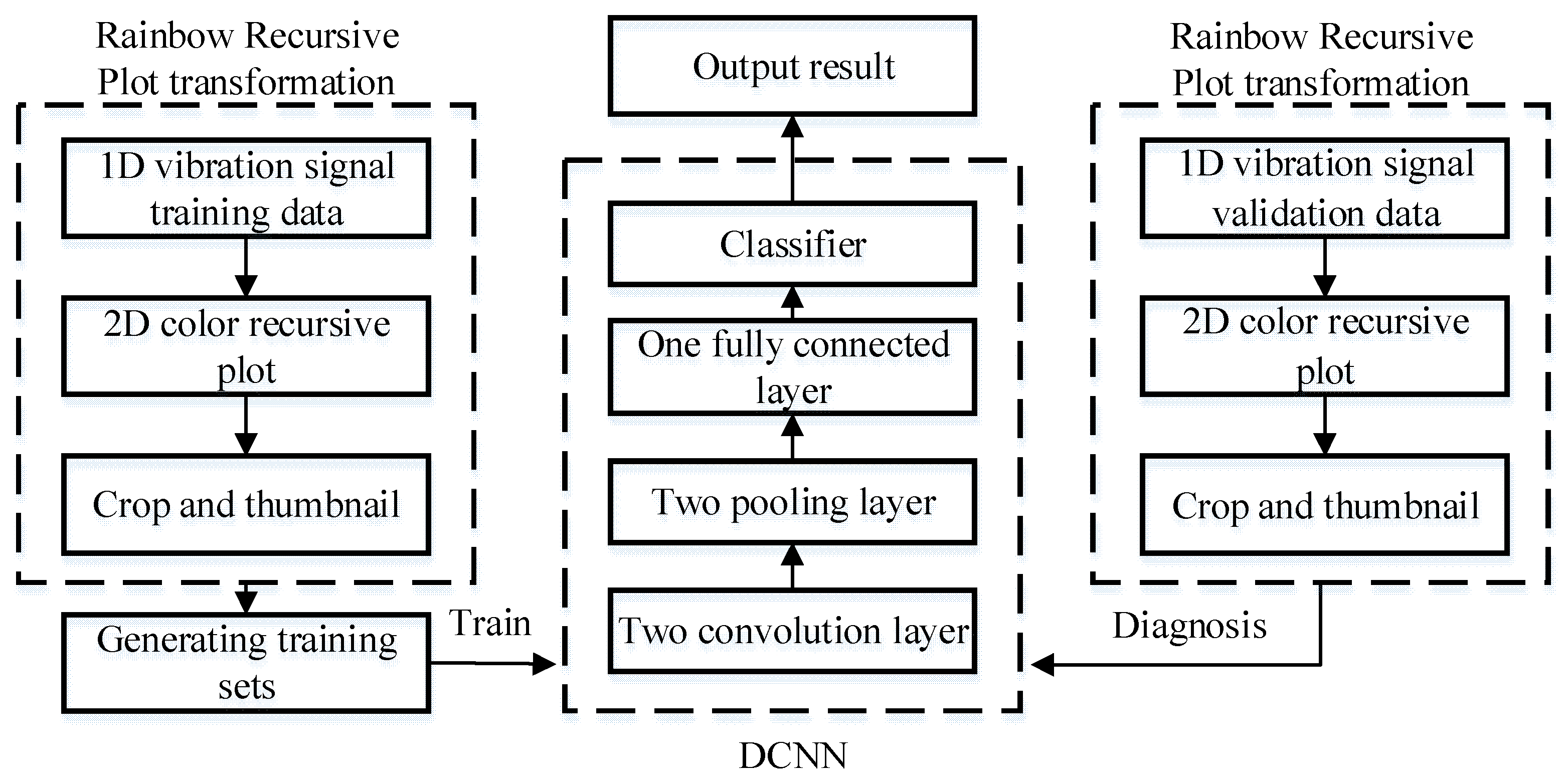
• We present a fast and effective feature extraction method. The RRP technology is used to change the one-dimensional vibration signal of bearing to a two-dimensional color image, which is transmitted to the optimized DCNN for learning and training, so as to complete the bearing fault diagnosis and recognition. The proposed method contains five successive steps. First, the one-dimensional vibration signals of bearing under normal and fault conditions are collected. Second, the one-dimensional vibration signal of bearing is converted into a two-dimensional color image by the RRP algorithm. Third, all rainbow recursive plots are preprocessed by appropriate cutting and abbreviation to improve the processing speed of the model. Fourth, the RRP dataset of bearing vibration is input to the optimized DCNN model for training. Fifth, the trained RRP-DCNN model is deployed to identify the bearing fault types.
• An improved CNN, RRP-DCNN-based bearing fault diagnosis method is proposed, which can use a little samples to perform a few learning times to obtain a high fault diagnosis accuracy rate.
• The data collected from the self-made test bench are input into RRP-DCNN for training and compared with traditional algorithms, the fault diagnosis method has been significantly improved.

The rest of this paper is organized as follows: A brief introduction of RRPs is provided in Section 2. The conversion of one-dimensional signals into two-dimensional color recursive plots, image preprocessing, and the specific construction of the convolutional neural network model will be introduced in Section 3. The experimental design and results are introduced in Section 4. The conclusions and future outlook is presented in Section 5.

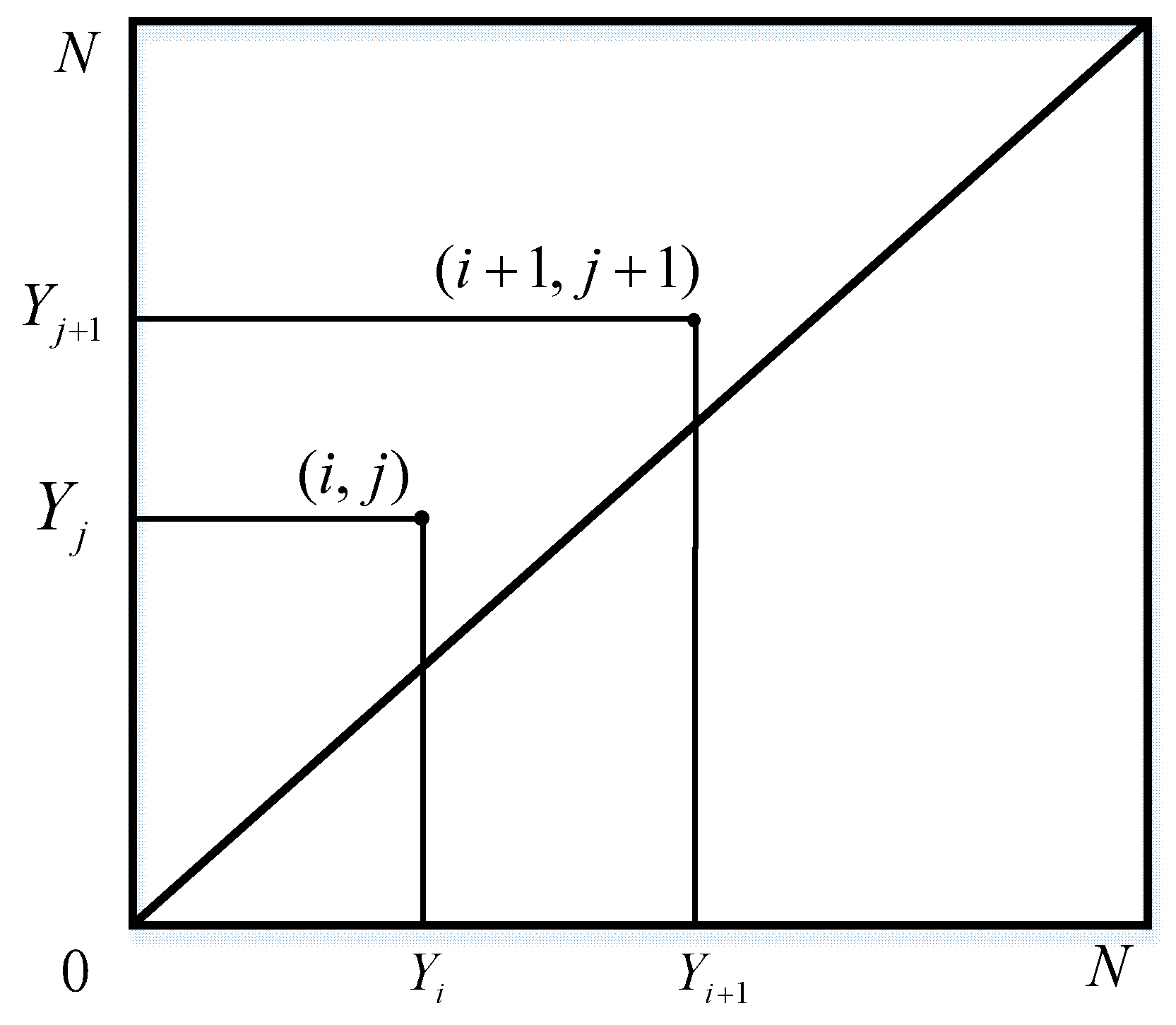
2. A Brief Introduction of RRPs

The vibration signals of most equipment are non-stationary and non-linear. More and more non-linear information processing technologies are used in the field of fault diagnosis, such as power spectrum analysis, multivariate time series analysis, and fractal dimension analysis. A recurrence plot method proposed by Eckmann et al., to reveal the dynamic characteristics of the system through binary image in 1987 [14,15]. A recursive plot is a good description method of mainstream shape, which is very suitable for the analysis of the characteristics of non-stationary fault state signals. The texture information of a recursive plot represents the relevant information of the system in time domain. From the perspective of recursive graph as a whole, it is the description of the global topological characteristics. The recursive plot can be used to describe the steady-state characteristics of the system. When the system is completely stable, the texture of the recursive plot is uniform. When the system is non-stationary, the detailed texture of the recursive plot will show relevant information in the time domain. As the instability increases, the detailed texture becomes more significant [16]. Recursive graphs can be used to analyze vibration signals under various equipment operating conditions. The calculation method for reconstruction is as follows [17]:

$$Y_i=\left\{x_i,x_{i+\tau },\cdots x_{i+\left(m-1\right)\tau }\right\},i=1,2,\cdots ,T-\left(m-1\right)\mathsf{\tau }$$

(1)

Among them, $T$ is the number of points in two-dimensional phase space, $X_i$, $i=1,2\dots n$ is time series, $m$ is bedded dimension, $\tau$ is delay constant.

The distance formula between the $j$-th point $Y_j$ and the $i$ -th point $Y_i$ is as follows [17]:

$$dist\left(i,j;m\right)=\frac{\left({{\displaystyle \sum }}_{k=0}^{m-1}\left|x_{i+k\tau }-x_{j+k\tau }\right|\right)}{{{\displaystyle \sum }}_{k=0}^{m-1}{x}_{i+k\tau }}$$

(2)

As shown in Figure 2, draw a square diagram with $N$ points on each side.$N$ represents the serial number of phase space, $R$ is a recursive matrix, and r is preset radius of the field. According to the results specified in the calculation [17]:

$$\left\{\begin{array}{c}{R}_{i,j} \mathrm{set} \mathrm{this} \mathrm{point} \mathrm{blank},\hspace{0.33em}\mathrm{when} \mathrm{dist}\left(i,j;m\right)>r\hfill \\ R_{i,j} \mathrm{set} \mathrm{this} \mathrm{as} \mathrm{a} \mathrm{solid} \mathrm{point},\hspace{0.33em}\mathrm{when} \mathrm{dist}\left(i,j;m\right)\le r\hfill \end{array}\right.$$

(3)

The drawing process of gray recurrence plot is introduced in detail in [17]. We use function RecurrencePlot( ) in the pyts.image module to generate rainbow recursive graph for feature extraction. Rainbow is a type of rainbow color mapping that maps data values to seven, namely colors violet, indigo, green, yellow, blue, red and orange, making it possible to display the changes in data more vividly. In function RecurrencePlot( ), rainbow color mapping is usually used to indicate the similarity between data, with closer points represented by more similar colors and distant points represented by less similar colors, making it easier to visualize the repeating patterns in time series data.

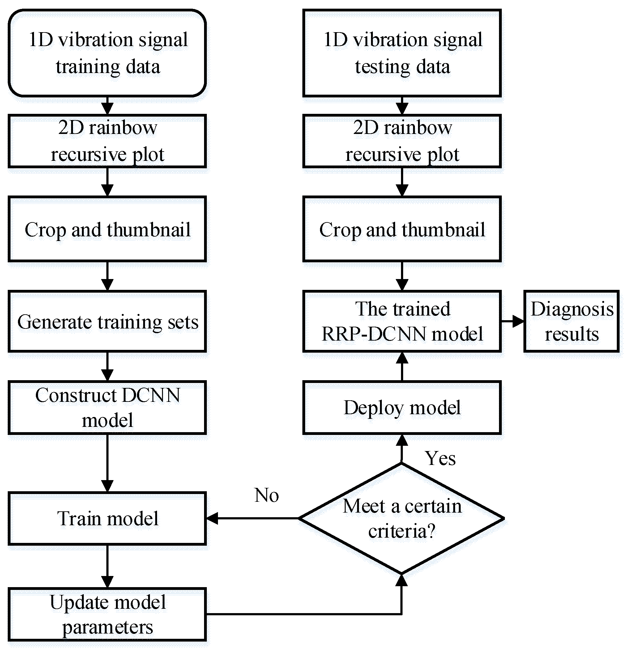
3. The Proposed RRP-DCNN Intelligent Diagnosis Method

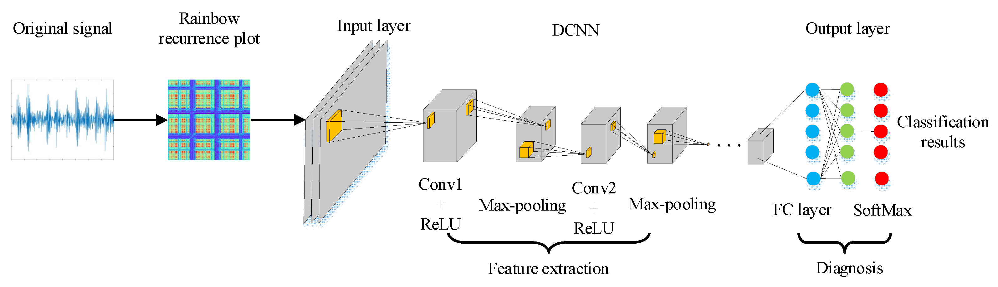
3.1. Overview of the Proposed RRP-DCNN Model

The architecture of the rotating machinery fault diagnosis method based on RRP-DCNN proposed in this article is shown in Figure 3.

With this method, a high accuracy rate in fault diagnosis can be achieved by utilizing a small number of samples and conducting only a limited number of learning iterations. This algorithm further improves the generalization ability of the fault diagnosis model, and is particularly suitable for the identification of fault types of non-stationary signals such as rotating machinery vibration.

First, the one-dimensional signal of vibration is converted into a two-dimensional color image through the RRP technology. The rainbow recursive plot has a good characterization function for non-stationary time series signals. Simple points and lines can show system dynamics characteristics well, and are very suitable for feature extraction in fault diagnosis of rotating machinery. In order to use the learning input of the convolutional neural network model, the recursive plot converted into a two-dimensional color image also needs to be preprocessed. Details of conversion and preprocessing based on a RRP are explained in Section 3.2.

In the field of image recognition, in order to increase the accuracy of the convolutional neural network model, it is generally performed deeper. Owing to the simple representation of the recursive plot, it is proposed to perform adaptive optimization on the basis of LeNet-5 [18,19]. The number of fully connected layers is reduced to form a deep convolutional neural network (DCNN) to improve the processing speed of the network model. In order to make the network model robust and avoid overfitting problems, the activation function ReLU. In order to further improve the generalization ability of the network model, the Dropout method is added after the pooling layer. In the classification stage, the softmax function is used to calculate the multi-objective probability distribution. Details about the DCNN are explained in Section 3.3.

3.2. RRP Conversion and Pretreatment

Taking the seven samples of all faults in the experimental data in Section 4.1 as examples, the whole process is shown in Figure 4.

The rainbow recursive plot acquisition and preprocessing process of the one-dimensional vibration signal of the rotary machinery based on the RRP-DCNN algorithm is as follows:

1.

Acquisition of one-dimensional vibration signals: The sampling frequency of the original rotary bearing signal is 12 kHz, that is, 12,000 points are collected per second, and the rotary machinery speed R = 1750 rpm, which is 1750 revolutions per minute. From this, the minimum number of sampling points $N_{min}$ for one revolution of the bearing is calculated as:

$$N_{min}=\frac{60F}{R}$$

(4)

In order to ensure the integrity of the sampling information, the actual number of sampling points is taken as N ≥ 1.5$N_{min}$, and we set N = 800.

2.

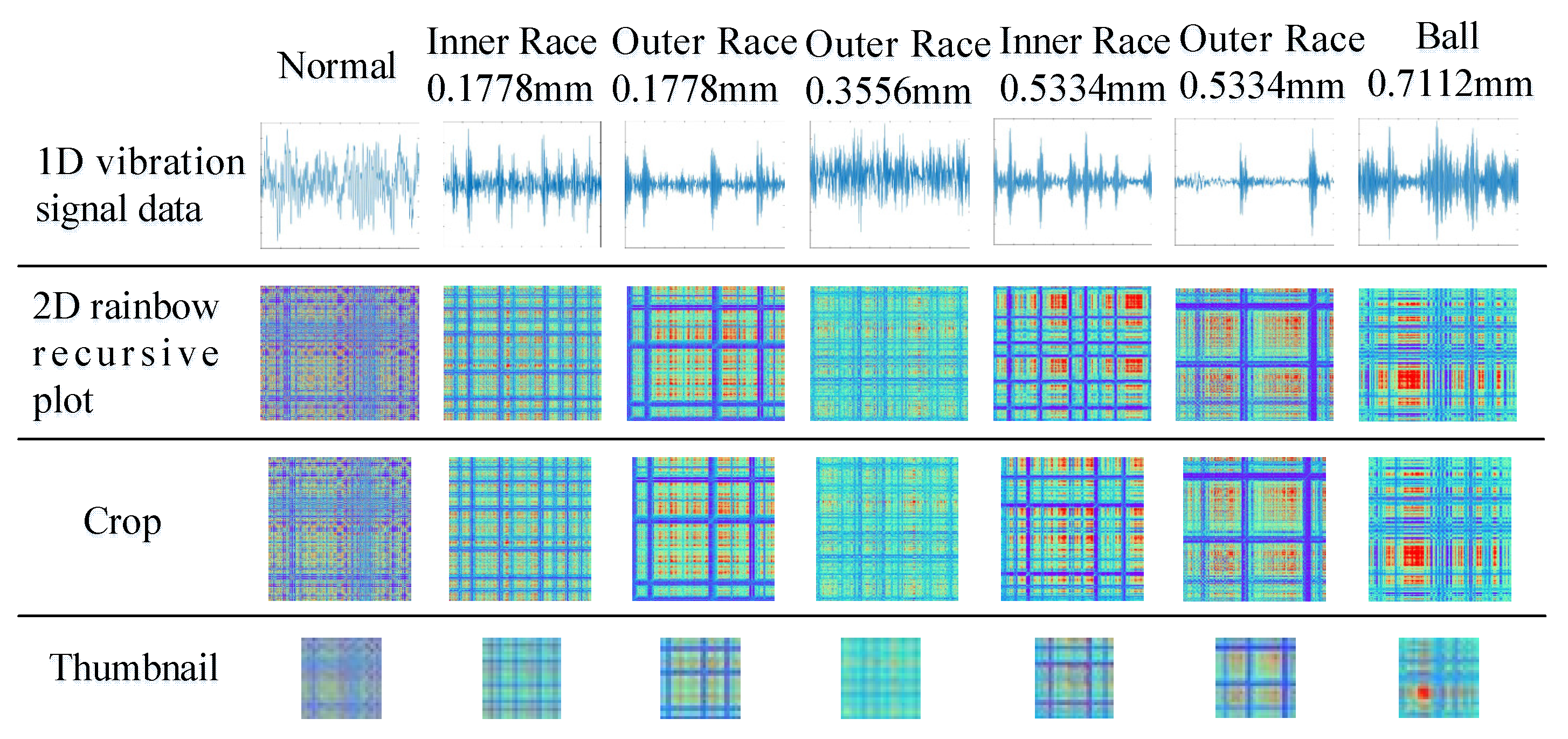
Draw a rainbow recursive plot: The vibration signals of the bearing under different working conditions are converted into a rainbow recursive plot using the method described in Section 2. The original rainbow recursive plot has a pixel size of 360 × 400.

3.

Crop the rainbow recursive plot: The pixels of the original rainbow recursive plot are large and odd, which is not conducive to the application of subsequent image recognition algorithms. The original rainbow recursive plot is cropped under the premise of ensuring the integrity of the information. Pixels of the cut rainbow recursive plot are 320 × 320.

4.

Abbreviate the recursive plot: The cut rainbow recursive plot can already be used for subsequent model training, but in the course of the experiment, the training speed is found to be very slow. After many experimental verifications, under the premise of ensuring a certain training effect, the cut rainbow recursive plot is further reduced to a 32 × 32 image by the function thumbnail ( ) in the PIL library.

5.

Mark the label: The preprocessed recursive thumbnails are labeled with the type of working conditions for subsequent learning and identification verification.

3.3. Design of a DCNN

Common CNNs in the field of image classification are: GoogleNet, VGG, AlexNet, LeNET-5, etc. These models are mainly for images with large samples and multiple categories. The number of convolutional layers that constitute a convolutional neural network is larger and deeper. The deeper the CNN is, the stronger the learning ability is. As the network becomes more complex, overfitting is easy to occur, and the training time will be longer. LeNet-5 is a classic convolutional neural network, which owns the advantages of shallow depth, fast training speed, and certain guarantee of accuracy [20]. It has been effectively applied in the industry. LeNet-5 contains a total of seven layers of structure—three convolutional layers, two max-pooling layers, one fully connected layer and one output layer [21,22]. For objects such as bearing fault diagnosis that pursues fewer samples and high fault recognition efficiency, CNNs need to balance the relationship between processing time and recognition accuracy when designing. This paper has made adaptive improvements on the basis of LeNet-5. Adding a Batch Normalization (BN) layer between convolutional and pooling layers can improve training efficiency. The structure is named a DCNN (Deep CNN). The specific structure of the DCNN is shown in

Table 1. DCNN structure parameters [17].

Number	Layer Type	Kernel Size	Step	Number of Kernels	Output Size
1	Conv	3 × 3	1	16	32 × 32 × 16
2	BatchNorm2d				32 × 32 × 16
3	MaxPool2d	2 × 2	2	16	16 × 16 × 16
4	Conv2d	3 × 3	1	32	16 × 16 × 32
5	BatchNorm2d				16 × 16 × 32
6	MaxPool2d	2 × 2	2	32	8 × 8 × 16
7	Fully connected	2048		1	2048 × 1
8	Fully connected	256		1	256 × 1
9	Softmax	7		1	7

adapted from [17].

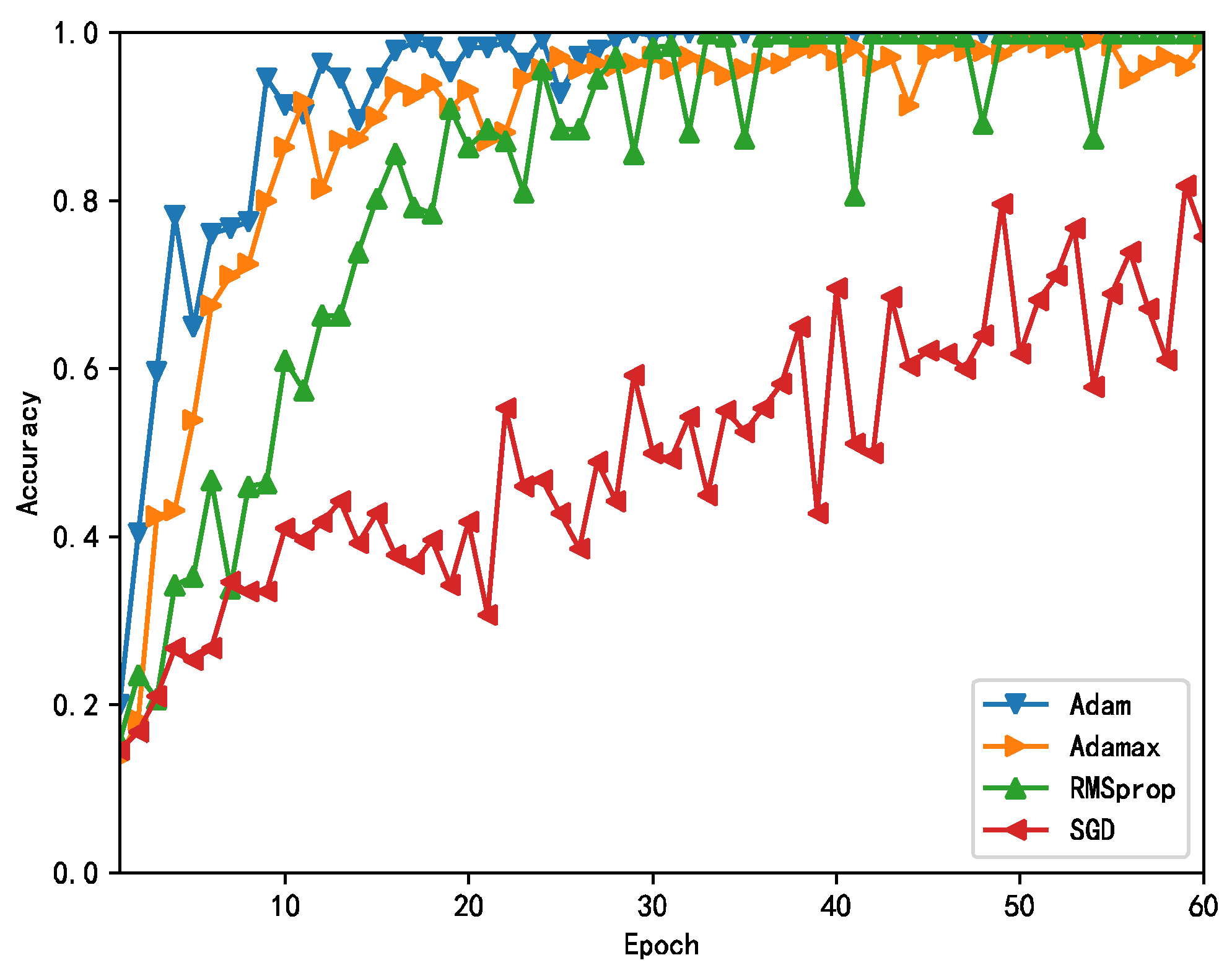
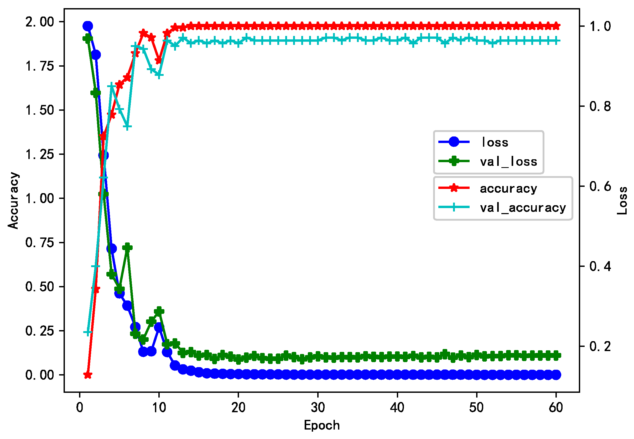
3.4. Training of the DCNN

The cross entropy loss function used to evaluate the CNN objective function is shown in Formula (5).

$$L=-\frac{1}{m} {{\displaystyle \sum }}_{k=1}^m{{\displaystyle \sum }}_j p_k^j\log q_k^j$$

(5)

Assuming the actual Softmax value of the CNN is $q$. The target distribution $p$ is an one-hot type vector, when the target category is $j$, $p^j=1$, otherwise $p^j=0$. Among them, $m$ represents the size of the input mini-batch, $q_k^j$ represents the probability that the $k$-th sample is calculated as the $j$-th class, $p_k^j$ is one-hot vector of the target domain sample tag.

The DCNN model uses the BP algorithm in the training process. Details of calculation process are explained in Section 3.3. In the process of training the DCNN model by choosing Stochastic Gradient Descent (SGD) in the BP algorithm, if the hyperparameters are not well selected, it is easy to fall into the local optimum during training. In addition, if the learning rate is not properly chosen, it will also fall into a local optimum. In order to solve the global optimum weight and minimize the value of the objective function, an optimization algorithm is required. Frequently used optimization algorithms include SGD with a fixed learning rate, the Adagrad algorithm with automatic learning rate change, the RMSprop algorithm with momentum, and adaptive moment estimation (Adam) optimization algorithm. After the experimental comparison in Section 4.3, this article chooses Adam as the model training optimization algorithm. In order to reduce the computational burden, dropout is added during the training phase. Due to prevent the occurrence of overfitting, regularization is used [23].

3.5. The RRP-DCNN Fault Diagnosis Process

The flow of the rotary machinery fault diagnosis method based on RRP-DCNN provided in this article is shown in Figure 5.

This method can adaptively extract the fault features from the one-dimensional vibration signal rainbow recursive plot. This method not only eases the burden of neural network model training, but also ensures the effective identification of faults. The algorithm is implemented as follows:

• Collect one-dimensional vibration signals of bearing under various working conditions such as normal and fault.
• Convert the one-dimensional vibration signal of the bearing into a two-dimensional rainbow recursive plots.
• Properly crop and abbreviate all rainbow recursive plots.
• Annotate fault classification labels and divide them into a training set and a test set with a ratio of 2:1.
• Input the training set to the built DCNN model, and perform iterative training to optimize network parameters until the trained model converges.
• Save and deploy the DCNN model.
• Collect the one-dimensional vibration signal of the rotary machinery under the new working condition. After processing according to steps (2) and (3), input to the DCNN model trained in step (6) to classify and identify the rotary machinery faults.

4. Experimental Results and Analysis

The target device is generally operating normally, and obtaining fault data is difficult. Comparing third-party standard databases with mainstream algorithms is a widely recognized and effective method.

4.1. Standard Dataset Validation

At present, the dataset of Case Western Reserve University (CWRU) Bearing Data Center utilized for motor bearing fault identification is the most widely used [24]. The vibration signal of the CURW dataset is collected by a 16-channel DAT recorder and processed into mat format by MATLAB. The sampling frequency of the data we chose is 12 kHz. There are four different speed states in this dataset, namely 1730 rpm, 1750 rpm, 1772 rpm, 1790 rpm, respectively. In each speed state, there are three kinds of faults: rolling fault (BA), inner ring fault (IF), outer ring fault (OF) and one normal condition (NO). Each type of failure has four different damage sizes, which are 0.18 mm, 0.36 mm, 0.53 mm and 0.71 mm. The position angle of the outer ring fault includes 0°, 90° and 180°. In this experiment, the rotating speed is 1750 rpm, the sampling frequency is 12 kHz. The vibration signal data of the drive end bearing are applied as the motor bearing fault set. The data composition is given in

Table 2. Description of rolling element bearing datasets.

Label	Fault Location	Damaged Degree/mm	Data Name	Train	Test
0	Normal	-	99.mat	40	20
1	Inner Race	0.1778	107.mat	40	20
2	Outer Race	0.1778	159.mat	40	20
3	Outer Race	0.3556	199.mat	40	20
4	Inner Race	0.5334	211.mat	40	20
5	Outer Race	0.5334	260.mat	40	20
6	Ball	0.7112	3007.mat	40	20

.

4.2. Parameters of the Proposed Model

In Section 2, the accuracy of using a recursive plot to describe system dynamics information mainly depends on the selection of phase space composition parameters: embedded dimension m and delay time τ. For the embedded dimension m, if m is too large, the amount of calculation will be increased and the influence of noise will be enlarged; if m is too small, the phase points of the phase space will cross in a certain area, resulting in the intersection area containing points in different parts of the phase space. For the delay time τ, if τ is too small, and the distance between $x\left(i\right)$ and $x\left(i+\tau \right)$ is as well close, the phase points are concentrated on the diagonal and it is difficult to distinguish. If τ is too large, $x\left(i\right)$ and $x\left(i+\tau \right)$ will be uncorrelated, and the phase points in the phase space will be distributed in two uncorrelated directions, which cannot truly reflect the law of system dynamics. In this paper, choosing m = 1, τ = 1 can achieve better experimental results. For other settings, please refer to Section 3.2.

In feature extraction and fault identification of the rotary machinery vibration signal using DCNN, the main parameters affecting the performance of the model are: CNN structure design, epoch, optimizer selection, learning rate and dropout. The structure of the DCNN has been introduced in Section 3.3. In the training stage, the upper limit of training times epoch is set to 60, the learning rate is set to 0.001, dropout is used in the full connection layer to suppress over fitting, and the dropout rate is set to 0.25. In the test phase, the dropout rate is set to 0 to ensure the diagnosis effect. The Adam algorithm is selected as the optimizer.

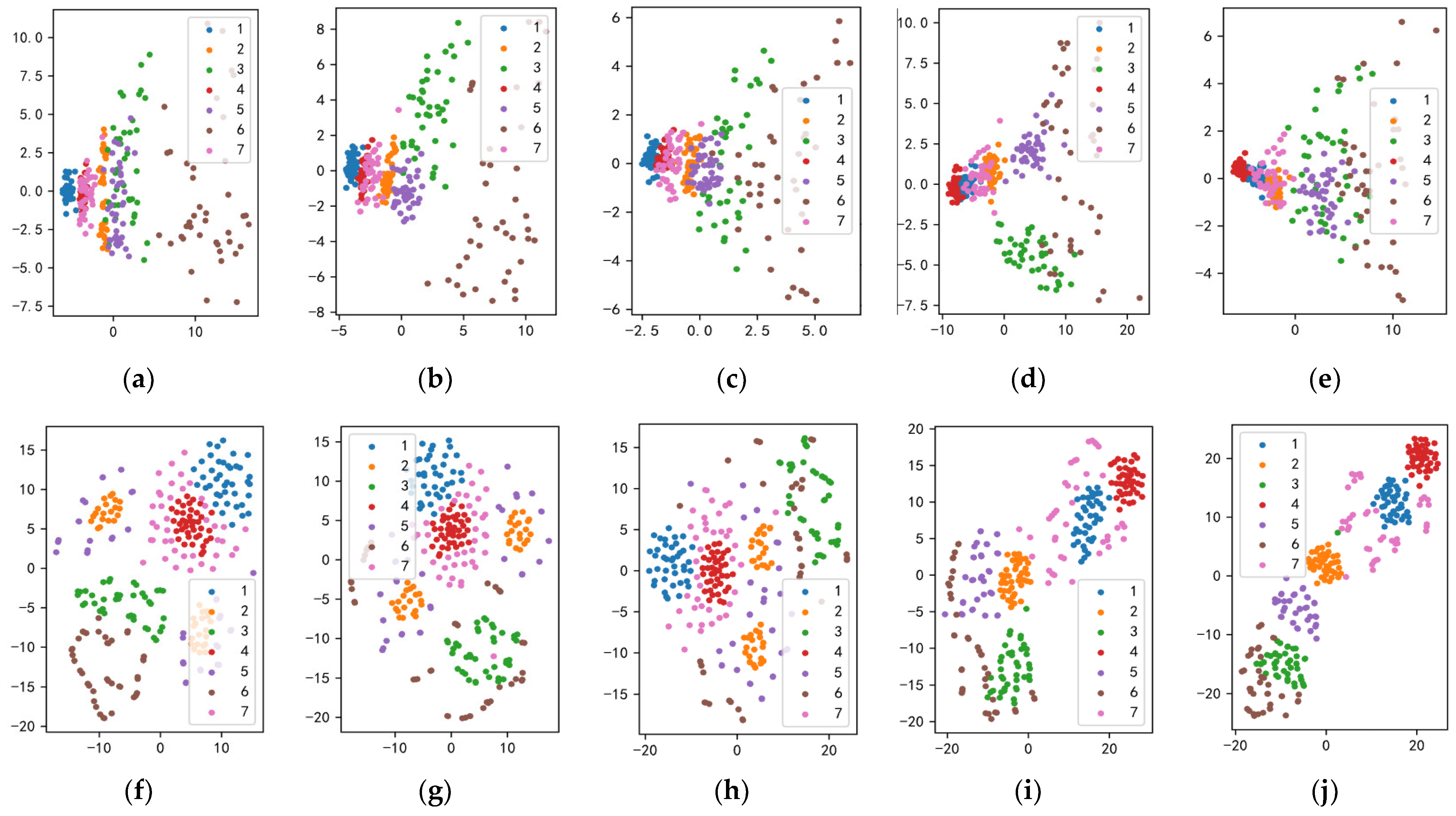
4.3. Fault Diagnosis Accuracy Assessment

Data of seven different bearing operating conditions with labels of 0–6 are selected to train the RRP-DCNN model. The number of training samples selected for each bearing operating condition is 40, and a total of 280 samples are used for model training. In addition, the number of verification samples selected for each bearing working condition is 20, and a total of 140 samples are used for model verification. In the model training stage, in order to select the best optimization algorithm, four algorithms of SGD, RMSprop, Adamax and Adam are used for experimental comparison. The comparison chart of the model training accuracy is shown in Figure 6. The training curves of SGD is the slowest. The convergence rate of RMSprop is faster, but it always fluctuates. The training curve of Adam is faster than that of Adamax, and the accuracy rate can be stabilized to 100%. Therefore, the Adam algorithm is selected as the optimizer.

In order to better observe the effect of the training process, the clustering effect visualization method is used for analysis. Figure 7 shows the clustering effect diagram of the training samples after the features of each layer of the CNN model are reduced to two dimensions.

The seven different colored dots in Figure 7 different working conditions. The first line of sub-figures 1 to 5 is the PCA dimensionality reduction method, and the second line of sub-figures 6 to 10 is the t-SNE method [25,26]. According to the observation of clustering results in Figure 7, the t-SNE dimensionality reduction method is clearer to view the effect of the training process than the PCA method. The t-SNE method in the second row of Figure 7 shows that as the number of network layers increases, samples gradually gather and become easier to divide, which makes it easier for the classifier to diagnose fault categories. Accordingly, the RRP-DCNN model has good adaptive fault feature extraction ability. As shown in Figure 8, the validation test accuracy approaches 100% after 20 iterations.

In order to verify the effectiveness of the method, input the verification sample data into the trained RRP-DCNN model. The result of diagnosis and recognition is automatically generated in the form of a confusion matrix, as shown in Figure 9. The horizontal axis represents actual operating conditions, and the vertical axis represents predicted operating conditions. The dark part of the diagonal line is the maximum probability value that the actual working condition is predicted to be correct. The other part is the probability value of the prediction error for other conditions. The predicted probability values from 0 to 100% correspond to the color map on the right. This type of classification result can be directly and clearly read out the classification accuracy rate of each working condition in the form of percentage from the graph. Due to the similarity in fault characteristics between fault 2 and fault 5, the recognition accuracy is relatively low. The recognition accuracy of fault 4 is 95%, while fault 2 has a lower recognition accuracy of 90%. This is in line with the intersection of the two fault clustering results in Figure 7. The accuracy of other fault identification is 100%. Overall, the fault diagnosis method based on RRP-DCNN is effective, achieving an average fault recognition accuracy of 97.86%.

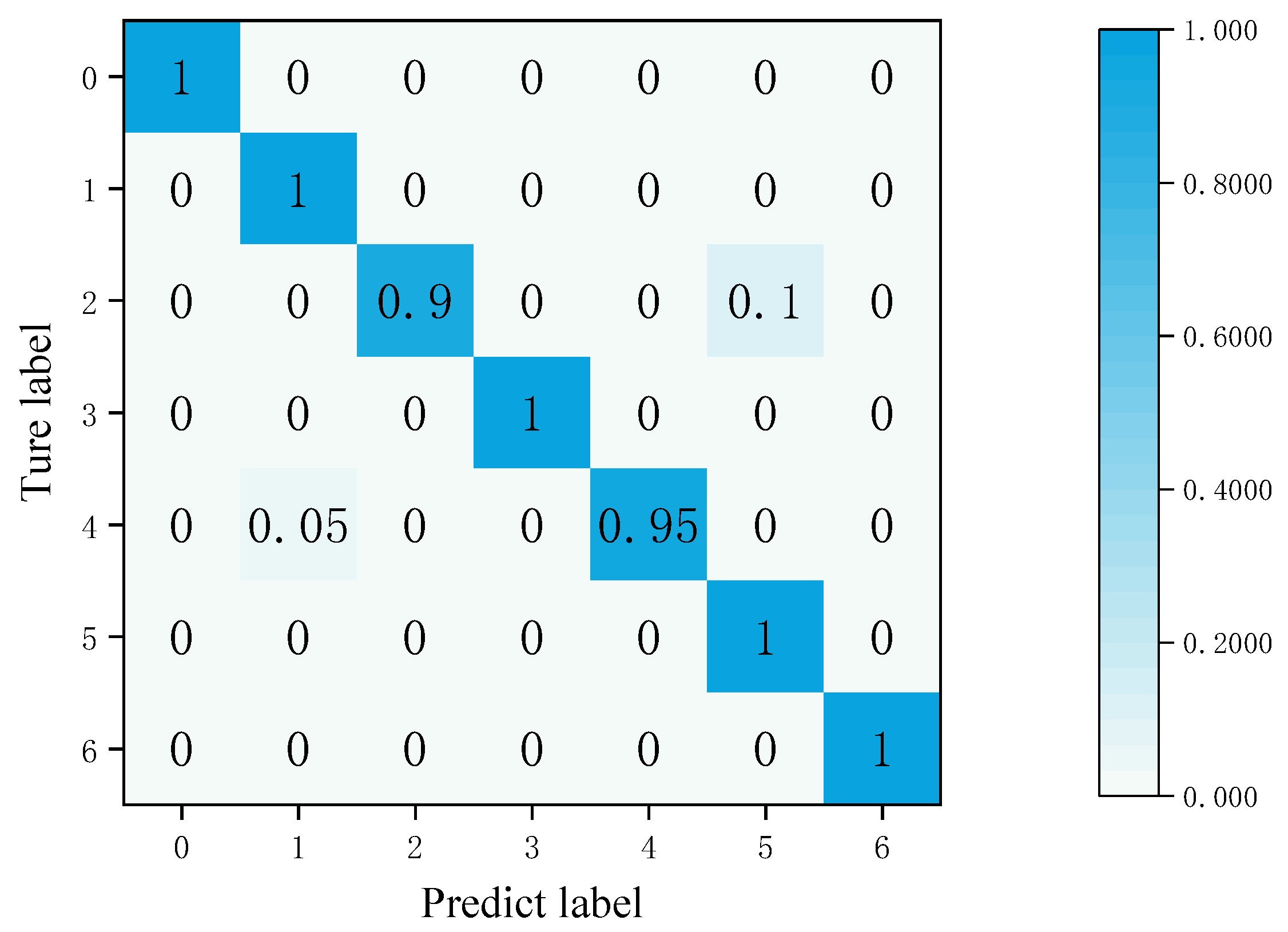
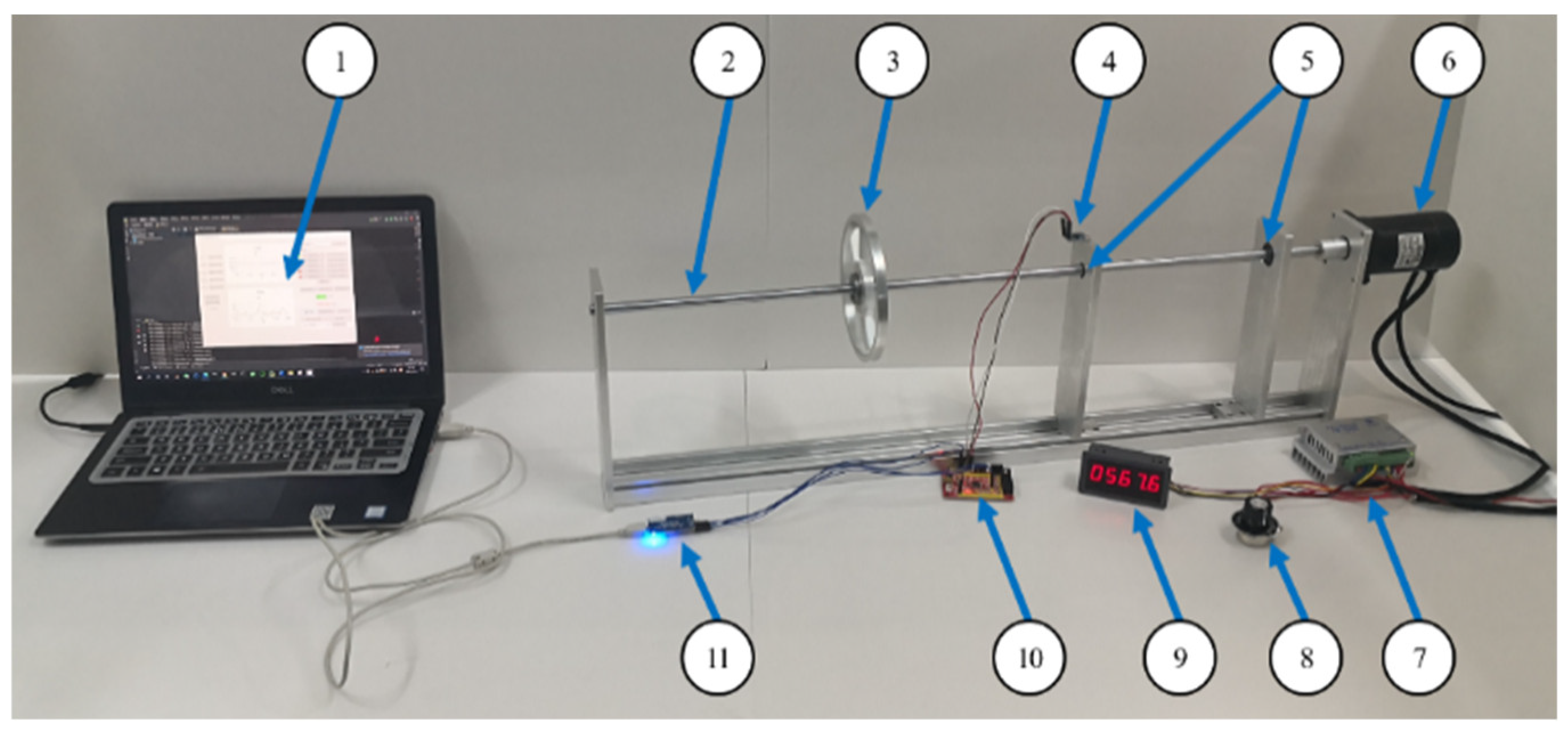
4.4. Self-Made Test Bench Verification

In order to further verify that the algorithm not only has good performance in the standard dataset, but also has good real-time and accuracy in engineering application, it is verified on-line. As shown in Figure 10, the experiment was conducted using the same platform as [27].

A fully functional self-made online fault diagnosis experimental platform is used to verify the effectiveness of the RRP-DCNN model. The ADXL335 vibration acceleration sensor with the sampling rate up to 1.6 kHz is selected for the experimental platform. The vibration acceleration sensor is installed on the bracket near the loading disk side, and the motor running speed is set to 500 rpm.

The center of gravity position of each loading disk is set differently, and the different center of gravity position can directly affect the imbalance state of the motor rotor. To simulate the operating conditions of the motor rotor, it can be achieved by switching different loading plates. Vibration signals of motor rotor faults under seven different working conditions are acquired as a self-dataset. The number of sampling points N = 220 is calculated according to Formula 10, and the subsequent data preprocessing is the same as that in Section 4.2. The data composition and division are shown in

Table 3. Description of self-data.

Label	Fault Type	Eccentric Wheels Specifications	Train	Test
0	Imbalance 1	Disk 1	70	30
1	Imbalance 2	Disk 2	70	30
2	Imbalance 3	Disk 3	70	30
3	Imbalance 4	Disk 4	70	30
4	Imbalance 5	Disk 5	70	30
5	Imbalance 6	Disk 6	70	30
6	Imbalance 7	Disk 7	70	30

.

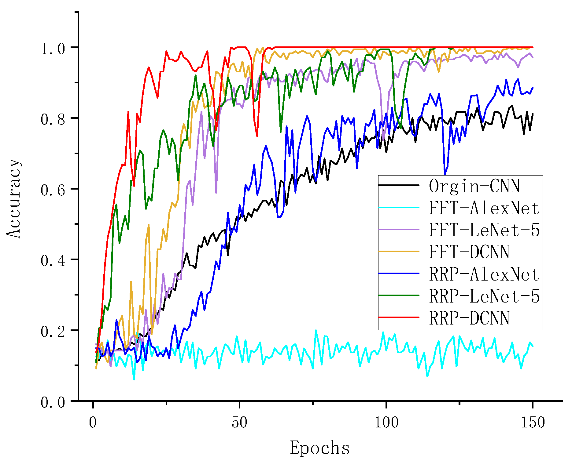
4.5. Method Comparison

In order to evaluate the recognition effect of the RRP-DCNN model, different algorithms are selected from the combination of the one-dimensional vibration signal preprocessing algorithm and the CNN model classifier for comparative experiments. The preprocessing algorithm includes FFT and the RRP algorithm in this paper. The deep learning model includes a CNN, AlexNet [28], LeNet-5 and a DCNN in this paper. The learning rate, epoch and other training parameters of the four deep learning models are consistent. Algorithms involved in comparative experiments include Orgin-CNN [29], FFT-AlexNet, FFT-LeNet-5, FFT-DCNN, RRP-AlexNet, RRP-LeNet-5, and RRP-DCNN. The algorithm Orgin-CNN directly uses the self-data original one-dimensional vibration signal as input. The input of this CNN is modified to adapt to the one-dimensional signal, and the others are consistent with the DCNN. FFT-AlexNet, FFT-LeNet-5, FFT-DCNN use self-data to convert the original one-dimensional vibration signal into a two-dimensional spectrogram as input [30]. RRP-AlexNet, RRP-LeNet-5 and RRP-DCNN use the preprocessing algorithm of this paper to transform the rainbow recursive plot as input. Figure 11 shows the test accuracy convergence curve in the process of training using the above seven algorithm models. First, compare and observe the four curves of Orgin-CNN, FFT-AlexNet, FFT-LeNet-5, and FFT-DCNN. The fastest convergence rate is FFT-DCNN, followed by FFT-LeNet-5. The origin CNN curve is slowly rising, while the FFT-AlexNet curve is still not obviously rising after 150 times of training. Therefore, the DCNN performs better when using the same FFT preprocessing algorithm. Then, RRP-AlexNet, RRP-LeNet-5 and RRP-DCNN were observed and compared. The fastest convergence rate is RRP-DCNN, followed by RRP-LeNet-5. The accuracy rate of RRP-DCNN is 100% after 50 times of training, RRP-LeNet-5 is 100% after 125 times of training, and RRP-AlexNet curve begins to rise obviously after 25 times of training, but it is still not stable after 150 times of training. Therefore, it is again confirmed that the DCNN model performs better. Compared with FFT-AlexNet and RRP-AlexNet curves, the RRP algorithm has more advantages in feature extraction. Compared with the FFT-DCNN and RRP-DCNN curves, the DCNN algorithm has more advantages in feature extraction speed and recognition accuracy. Overall, RRP-DCNN is higher than other algorithms in terms of convergence speed and accuracy after 150 times of training, which shows that the method in this paper is efficient in motor rotor fault diagnosis.

The self-data training set is input into the model of various algorithms for 150 iterations training, and the training time is recorded. In the self-data test set, 45 data samples are randomly selected for classification and recognition in each type of working condition, and the recognition accuracy of each algorithm model and the average recognition time of a single sample are recorded, as shown in

Table 4. Experiment results.

	Condition Label							Results
Algorithm	0	1	2	3	4	5	6	Training Time (s)	Identification Time (s)	Average Accuracy (%)
Orgin-CNN	46.7	26.7	93.3	60.0	93.3	33.3	93.3	3.2588186	0.0003233	63.81
FFT-AlexNet	0.0	0.0	100.0	0.0	0.0	0.0	0.0	135.9444344	0.0023147	14.29
FFT-LeNet-5	100.0	93.3	100.0	100.0	100.0	73.3	100.0	27.3925648	0.0006411	95.24
FFT-DCNN	86.7	93.3	100.0	100.0	100.0	86.7	100.0	23.1145761	0.0005811	95.24
RRP-AlexNet	91.1	100.0	55.6	44.4	93.3	82.2	88.9	179.5841630	0.0019357	79.37
RRP-LeNet-5	100.0	100.0	97.8	88.9	97.8	100.0	88.9	35.3096957	0.0006984	96.19
RRP-DCNN	100.0	97.8	97.8	100.0	100.0	100.0	88.9	30.0779228	0.0006553	97.78

.

It can be seen from Table 4 that RRP-AlexNet has the greatest training time and recognition time, followed by FFT-AlexNet. This is caused by the deeper number of layers in the AlexNet network. Origin-CNN has the shortest time and recognition time, but the average diagnostic accuracy is only 63.81%. This shows that the ability to directly use the original signal for feature extraction is insufficient. The training time and recognition time of FFT-LeNet-5 is slightly longer than that of FFT-DCNN. This is due to the fact that the LeNet-5 network has more layers than the DCNN. Since the DCNN and LeNet-5 models are relatively close, their recognition accuracy is also 95.24% when the number of training times is sufficient.

Compared with FFT-LeNet-5 and FFT-DCNN, RRP-LeNet-5 has slightly less training time and recognition time, but the recognition accuracy rate is improved to 96.19%. This shows that the RRP is more advantageous than FFT in feature extraction efficiency. Compared with RRP-LeNet-5, RRP-DCNN has less training and recognition time, and the average correct rate of fault diagnosis can reach 97.78%. From the comprehensive performance of the experiment, RRP-DCNN has the highest efficiency, which is more in line with the actual needs of engineering.

5. Conclusions

In this study, a fast and effective feature extraction method was proposed. The recursive plot technology was used to convert the one-dimensional vibration signal of rotary machinery into a two-dimensional color image, which was transmitted to the optimized DCNN for learning and training, so as to complete the rotary machinery fault diagnosis and recognition. The effectiveness of this method was first verified by experiments on the CWRU dataset. The relationship between the optimization algorithm and the diagnosis results in the training process was studied. The correlation between the clustering effect of each layer output of the RRP-DCNN model and the recognition result of confusion matrix was investigated and discussed. Moreover, the data acquired from the self-made online test bench were utilized for training the RRP-DCNN model. Compared with the traditional algorithm in the accuracy and time efficiency of fault diagnosis identification, the efficiency of the algorithm was further verified. The 2D CNN used in this article cannot adaptively adjust the structure and network parameters once the model is fixed. If a “dynamic feedback” mechanism is added, the network model can be optimized based on the characteristics of the data, truly realizing an artificial intelligence method for unmanned parameter adjustment, and improving the generalization performance and robustness of fault diagnosis methods.

References

1. Arellano-Espitia, F.; Delgado-Prieto, M.; Martinez-Viol, V.; Saucedo-Dorantes, J.J.; Osornio-Rios, R.A. Deep-Learning-Based Methodology for Fault Diagnosis in Electromechanical Systems. Sensors 2020, 20, 3949. [Google Scholar] [CrossRef] [PubMed]
2. Zhang, S.; Zhang, S.; Wang, B.; Habetler, T.G. Deep Learning Algorithms for Bearing Fault Diagnostics—A Comprehensive Review. IEEE Access 2020, 8, 29857–29881. [Google Scholar] [CrossRef]
3. Yu, Y.; Liang, S.; Samali, B.; Nguyen, T.N.; Zhai, C.; Li, J.; Xie, X. Torsional capacity evaluation of RC beams using an improved bird swarm algorithm optimised 2D convolutional neural network. Eng. Struct. 2022, 273, 115066. [Google Scholar] [CrossRef]
4. Yu, Y.; Rashidi, M.; Samali, B.; Mohammadi, M.; Nguyen, T.N.; Zhou, X. Crack detection of concrete structures using deep convolutional neural networks optimized by enhanced chicken swarm algorithm. Struct. Health Monit. 2022, 21, 2244–2263. [Google Scholar] [CrossRef]
5. Skowron, M.; Orlowska-Kowalska, T.; Wolkiewicz, M.; Kowalski, C.T. Convolutional Neural Network-Based Stator Current Data-Driven Incipient Stator Fault Diagnosis of Inverter-Fed Induction Motor. Energies 2020, 13, 1475. [Google Scholar] [CrossRef]
6. An, Z.; Li, S.; Xin, Y.; Xu, K.; Ma, H. An intelligent fault diagnosis framework dealing with arbitrary length inputs under different working conditions. Meas. Sci. Technol. 2019, 30, 125107. [Google Scholar] [CrossRef]
7. Zhang, W.; Peng, G.; Li, C.; Chen, Y.; Zhang, Z. A New Deep Learning Model for Fault Diagnosis with Good Anti-Noise and Domain Adaptation Ability on Raw Vibration Signals. Sensors 2017, 17, 425. [Google Scholar] [CrossRef]
8. Yang, J.; Yin, S.; Chang, Y.; Gao, T. A Fault Diagnosis Method of Rotating Machinery Based on One-Dimensional, Self-Normalizing Convolutional Neural Networks. Sensors 2020, 20, 3837. [Google Scholar] [CrossRef]
9. Islam, M.M.M.; Kim, J. Automated bearing fault diagnosis scheme using 2D representation of wavelet packet transform and deep convolutional neural network. Comput. Ind. 2019, 106, 142–153. [Google Scholar] [CrossRef]
10. Zhou, C.; Zhang, W. A New Process Monitoring Method Based on Waveform Signal by Using Recurrence Plot. Entropy 2015, 17, 6379–6396. [Google Scholar] [CrossRef]
11. Yuan, L.; Lian, D.; Kang, X.; Chen, Y.; Zhai, K. Rolling Bearing Fault Diagnosis Based on Convolutional Neural Network and Support Vector Machine. IEEE Access 2020, 8, 137395–137406. [Google Scholar] [CrossRef]
12. Koh, D.; Jeon, S.; Han, S. Performance Prediction of Induction Motor Due to Rotor Slot Shape Change Using Convolution Neural Network. Energies 2022, 15, 4129. [Google Scholar] [CrossRef]
13. Garcia-Ceja, E.; Uddin, M.Z.; Torresen, J. Classification of Recurrence Plots’ Distance Matrices with a Convolutional Neural Network for Activity Recognition. Procedia. Comput. Sci. 2018, 130, 157–163. [Google Scholar] [CrossRef]
14. Hirata, Y. Recurrence plots for characterizing random dynamical systems. Commun. Nonlinear Sci. Numer. Simul. 2021, 94, 105552. [Google Scholar] [CrossRef]
15. Marwan, N.; Carmen Romano, M.; Thiel, M.; Kurths, J. Recurrence plots for the analysis of complex systems. Phys. Rep. 2007, 438, 237–329. [Google Scholar] [CrossRef]
16. Shi, Y.; Guo, Y.; Yao, T.; Liu, Z. Sea-Surface Small Floating Target Recurrence Plots FAC Classification Based on CNN. IEEE Trans. Geosci. Remote Sens. 2022, 60, 5115713. [Google Scholar] [CrossRef]
17. Wang, X.; Wang, X.; Zhang, X.; Chen, Q. Motor Fault Diagnosis Under Variable Working Conditions Based on Two-Dimensional Time Series and Transfer Learning. In Proceedings of the 25th International Conference on Electrical Machines and Systems (ICEMS), Chiang Mai, Thailand, 2 December 2022; pp. 1–5. [Google Scholar]
18. Zhang, Z. From Artificial Neural Networks to Deep Learning: A Research Survey. J. Phys. Conf. Ser. 2020, 1576, 12030. [Google Scholar] [CrossRef]
19. Wang, Y.; Li, F.; Sun, H.; Li, W.; Zhong, C.; Wu, X.; Wang, H.; Wang, P. Improvement of MNIST Image Recognition Based on CNN. IOP Conf. Ser. Earth Environ. Sci. 2020, 428, 12097. [Google Scholar] [CrossRef]
20. Xu, G.; Liu, M.; Jiang, Z.; Shen, W.; Huang, C. Online Fault Diagnosis Method Based on Transfer Convolutional Neural Networks. IEEE Trans. Instrum. Meas. 2020, 69, 509–520. [Google Scholar] [CrossRef]
21. Wang, K.; Chen, C.; He, Y. Research on pig face recognition model based on keras convolutional neural network. IOP Conf. Ser. Earth Environ. Sci. 2020, 474, 32030. [Google Scholar] [CrossRef]
22. Wen, L.; Li, X.; Gao, L.; Zhang, Y. A New Convolutional Neural Network-Based Data-Driven Fault Diagnosis Method. IEEE Trans. Ind. Electron. 2018, 65, 5990–5998. [Google Scholar] [CrossRef]
23. Chen, Z.; Li, C.; Sanchez, R. Gearbox Fault Identification and Classification with Convolutional Neural Networks. Shock Vib. 2015, 2, 390134. [Google Scholar] [CrossRef]
24. Gao, S.; Xu, L.; Zhang, Y.; Pei, Z. Rolling bearing fault diagnosis based on intelligent optimized self-adaptive deep belief network. Meas. Sci. Technol. 2020, 31, 55009. [Google Scholar] [CrossRef]
25. Xue, J.; Chen, Y.; Li, O.; Li, F. Classification and identification of unknown network protocols based on CNN and T-SNE. J. Physics. Conf. Ser. 2020, 1617, 12071. [Google Scholar] [CrossRef]
26. Garg, I.; Panda, P.; Roy, K. A Low Effort Approach to Structured CNN Design Using PCA. IEEE Access 2020, 8, 1347–1360. [Google Scholar] [CrossRef]
27. Wang, X.; Wang, X.; Chen, Q.; Zhang, X. Design of Experimental Platform for Motor Fault Diagnosis Based on Embedded System and Shallow Neural Network. In Proceedings of the 25th International Conference on Electrical Machines and Systems (ICEMS), Chiang Mai, Thailand, 2 December 2022; pp. 1–5. [Google Scholar]
28. Ma, P.; Zhang, H.; Fan, W.; Wang, C.; Wen, G.; Zhang, X. A novel bearing fault diagnosis method based on 2D image representation and transfer learning-convolutional neural network. Meas. Sci. Technol. 2019, 30, 55402. [Google Scholar] [CrossRef]
29. Zhang, X.; Han, P.; Xu, L.; Zhang, F.; Wang, Y.; Gao, L. Research on Bearing Fault Diagnosis of Wind Turbine Gearbox Based on 1DCNN-PSO-SVM. IEEE Access 2020, 8, 192248–192258. [Google Scholar] [CrossRef]
30. Xiao, Y.; Wei, X.Z. Specific emitter identification of radar based on one dimensional convolution neural network. J. Phys. Conf. Ser. 2020, 1550, 32114. [Google Scholar] [CrossRef]
Figure 1. The block diagram of the proposed method.
Energies 16 04357 g001
Figure 2. Drawing process of recurrence plot [17].
Energies 16 04357 g002
Figure 3. Architecture of the proposed RRP-DCNN method.
Energies 16 04357 g003
Figure 4. RRP conversion and preprocessing.
Energies 16 04357 g004
Figure 5. Fault diagnosis process based on RRP-DCNN.
Energies 16 04357 g005
Figure 6. Comparison chart of the accuracy of four optimization algorithms.
Energies 16 04357 g006
Figure 7. Feature visualization of training samples: (a) PCA-origin; (b) PCA-conv_1; (c) PCA-maxplooing_1; (d) PCA-conv_2; (e) PCA-maxplooing_2; (f) T-SNE-origin; (g) T-SNE -conv_1; (h) T-SNE-maxplooing_1; (i) T-SNE -conv_2; (j) T-SNE -maxplooing_2.
Energies 16 04357 g007
Figure 8. Procedures of the RRP-DCNN training and validation.
Energies 16 04357 g008
Figure 9. Confusion matrix of RRP-DCNN fault recognition.
Energies 16 04357 g009
Figure 10. Fault diagnosis test bench. (1) Upper computer. (2) Shaft. (3) Loading disk. (4) Acceleration sensor. (5) Bearing. (6) Motor. (7) Motor driver. (8) Speed adjustment button. (9) Speed display. (10) Data acquisition board. (11) Serial communication [27].
Energies 16 04357 g010
Figure 11. Procedures of the self-made test bench training.
Energies 16 04357 g011