Supercapacitor Constant-Current and Constant-Power Charging and Discharging Comparison under Equal Boundary Conditions for DC Microgrid Application

Abstract

This work analyzes and compares the differences in efficiency between supercapacitor constant-current and constant-power charging under the same boundary conditions, i.e., charging from the same initial voltage to the same final voltage in equal charging times in both variants. Similarly, supercapacitor constant-current and constant-power discharging are compared under the same boundary conditions, i.e., discharging from the same initial voltage to the same final voltage in equal discharging times for both variants. The study included calculations and virtual simulations based on the most frequently used equivalent RC model of supercapacitors. As a result, theoretical calculations and simulations with the RC model confirmed that constant-current charging/discharging is more efficient than constant-power charging/discharging. The results show that this difference is usually not higher than 1%. Practical experiments confirm an almost equal efficiency of both strategies, but it was difficult to validate exactly such small, theoretically calculated differences. Overall, from a practical point of view, the two charging/discharging methods can be considered as close, and nearly equal in terms of efficiency.

1. Introduction

DC voltage is widely used, as most electrical energy consumers are supplied by DC current, e.g., lighting, motor drives, etc. [1]. Three-phase AC motors are most often supplied via a DC link starting with an AC-DC rectifier and ending with a DC-AC inverter. In addition, DC lines reduce the number of conversion stages, such as AC-DC converters and filters. These advantages are contributing to the development of DC microgrids. Moreover, a regenerative electric drive connected to the DC grid can supply power to other consumers connected to the same DC grid during its deceleration mode [2]. Energy efficiency can be significantly improved by installing energy storage systems (ESS) on the DC grid. If no other consumer requires regenerated energy at the moment, it is economical to store this energy in ESS for re-use when needed instead of dissipating it in heat [3].

In the last two decades, so-called ultracapacitors or supercapacitors (SCs) have been increasingly used for electrical energy storage in many high-power applications due to their much higher capacitance compared to conventional capacitors, allowing them to store significantly larger amounts of energy [4,5]. While batteries still have a higher energy density, SCs have a higher power density due to which they can be charged and discharged relatively rapidly. SCs are therefore useful for applications such as electric vehicle drives, which regenerate electrical power during braking mode, and this regenerated power can be stored for re-use in the next acceleration mode, thus reducing the full consumption of electricity from a power supply substation in the case of public electric transport connected to an overhead grid [6]. Power recovery is topical also in equipment used in the production industry, including industrial robots [2,7,8]. In the above mentioned situations, the use of SC ESS is an optimal choice to reduce energy consumption.

In practice, bidirectional DC-DC converters connected between microgrid DC bus and SC ESS ensure these charging/discharging processes. Certain types of converters are designed to provide a constant charge/discharge voltage but tend to have limited ranges of usable voltage values. Larger differences between the source voltage and the SC circuit voltage might lead to higher current peaks, thus reducing the efficiency [9,10]. Several papers summarize control methods for different applications: [11,12,13], for electrical vehicles [14], and for DC microgrid application [15,16,17,18]. Most common control techniques other than constant-voltage control are constant-current and constant-power control methods, as SCs are quite commonly used in constant current and constant power charging and discharging applications [19,20]. Therefore, the focus of this paper is SC constant-current and constant-power charging and SC constant-current and constant-power discharging.

In planning the implementation of an SC ESS, preliminary calculations must be carried out to predict its performance under the given conditions and whether it will be able to fulfil its energy storage and supply tasks. The corresponding calculations and/or virtual simulations are carried out using SC mathematical models. The most widely used, the so-called RC model, is the simplest but does not guarantee complete accuracy, which is why various other models have been developed [21]. In [22], SC models are classified into four categories: electrochemical, equivalent circuit, intelligent and fractional order [23]. It is also worth mentioning models such as the Zubieta model [24], Faranda model [25] and two RC branches’ circuit model [26,27]. In [28], a comparison of the accuracy of three different models—RC circuit, two-branch circuit and multi-branch circuit—was made and it was found that the simplified RC model shows higher error compared to the other more complex models. A closer look at the result graphs suggests that the RC circuit model is slightly over 5% more inaccurate than the other two models. Therefore, the simplified RC circuit model can be considered as an acceptable model for planning and calculation of large SC ESSs [29] and many other applications.

Unlike SC constant-current charging/discharging, the analysis of the constant-power charging/discharging processes involves more complex differential equations. Therefore, various studies have been conducted on the operation of SCs’ constant-power modes. For example, refs. [30,31,32] describe the process of SC constant-power discharging by calculating the electrical parameters—current, internal voltage, external voltage etc.—using the Lambert W function in real time. The research was performed with theoretical calculations and simulations based on an RC circuit.

Nevertheless, a detailed comparison of SC constant-current charge/discharge and constant-power charge/discharge under the same boundary conditions, that include initial SC voltage, final SC voltage, charge time and discharge time based on the RC circuit model, has not been made in the literature so far. The insights gained from this work can therefore be useful for both researchers and engineers. The article presents fundamental research supported with simulations and experiments proving that, for an RC circuit, charging/discharging an SC with constant current is more efficient than charging/discharging with constant power when both options have the same boundary conditions, but this difference is typically less than 1% and varies with both the chosen boundary conditions and the internal resistance of the SC. As SCs are widely used globally, this difference, although numerically small, can have a certain impact on both the overall energy consumption and the lifetime of separate SC cells.

2. Conditions for Supercapacitor Charging and Discharging Comparison

Deciding to compare the charging of an SC circuit from a specified initial voltage to a specified final voltage at a strictly defined time with constant current and constant supplied power, an assumption might arise even prior to such experimental comparison that both of these charging variants should be identical in terms of efficiency, since the charging conditions for both options are the same: the voltage at the beginning of charging; the voltage at the end of charging; the time of charging. The same assumption might also arise prior to comparing a SC circuit discharging with constant current and constant power under equal discharging conditions. Through calculations and experimental simulations, the present work describes the rationale for proving that constant-current charging is not identical in terms of efficiency to constant-power charging, and constant-current discharging is not identical in terms of efficiency to constant-power discharging.

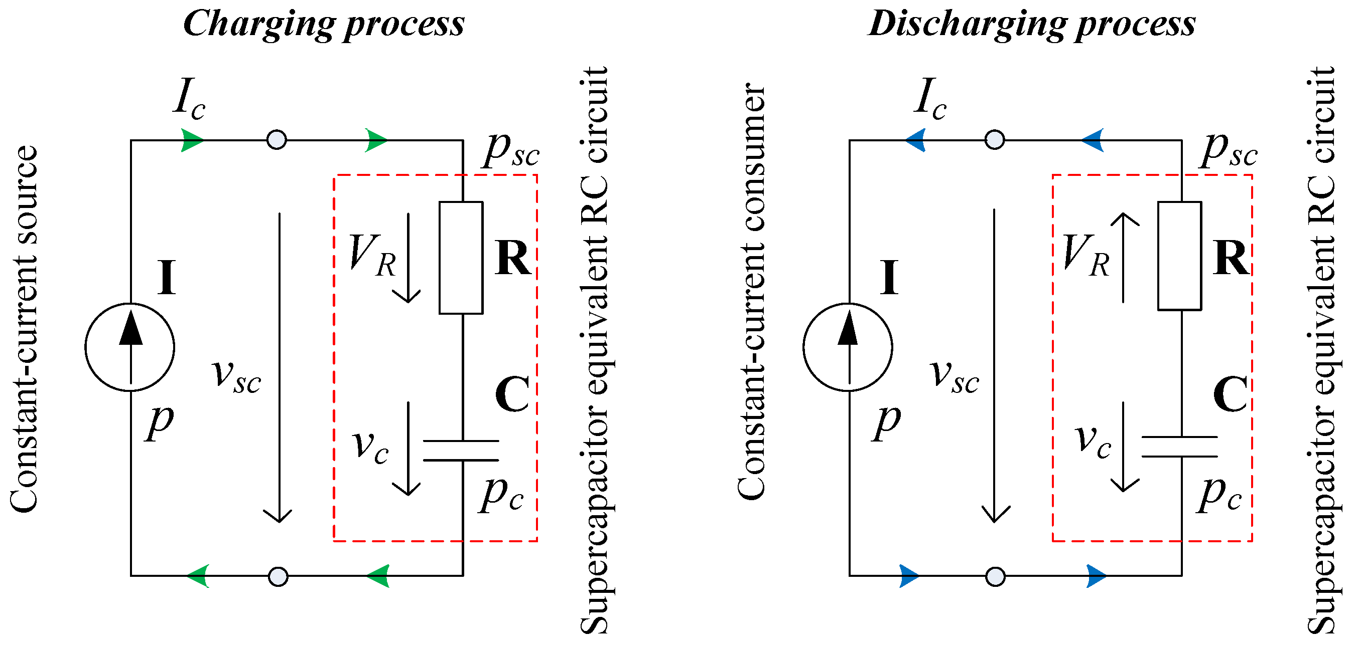
For the calculations and their confirmatory simulation results, a simplified equivalent model of a SC circuit was used—the RC circuit shown in Figure 1, consisting of a capacitor C simulating the full capacitance and a resistor R simulating the full active internal resistance. In RC circuits, there is often another resistor in parallel with C to simulate self-discharge losses [33], which are relevant over longer time periods, so this was not considered in further work. Although capacitance decreases and resistance increases during the lifetime of SCs, these parameters were assumed to be constant during any given charge/discharge cycle. The actual electrical processes of the SC differ slightly from the simplified RC circuit due to various electrical, chemical, and thermal processes. However, from the operation graphs of different SC models in [28], it can be concluded that the error of the RC model compared to more complex and accurate models is generally slightly higher than 5%. It was therefore decided to use an RC circuit model for all calculations and virtual simulations. Before starting the work, a certain SC cell with known R and C needs to be selected, based on which the corresponding simulations will be performed.

Calculations, simulations, and experiments were performed on a SC circuit consisting of 20 series-connected SC cells Maxwell BCAP0450 P270 S18 that will be used as energy storage for a 48 V DC microgrid. According to the manufacturer’s technical documentation, the capacitance of one such cell is C = 450 F, internal resistance R = 2.8 mΩ and the maximum voltage V_C = 2.7 V. Therefore, for a circuit with 20 series-connected cells, C = 22.5 F, R = 0.056 Ω and V_C = 54 V, respectively. Comparisons between two SC charging methods—constant-current and constant-power charging—were made by charging the SC circuit from the initial voltage V_C1 to the final voltage V_C2 at equal time durations t. Afterwards, comparisons between the two SC discharging methods—constant-current and constant-power discharging—were made by discharging the SC circuit from the initial voltage V_C2 to the final voltage V_C1, that was previously the case before charging, at equal time duration t, at which the charging was previously performed. Experimental computer simulations of the charging/discharging of the given SC circuit were performed using the Matlab/Simulink environment, entering pre-calculated input parameters.

The initial state-of-charge voltage of the SC circuit was assumed to be half of the maximum, i.e., V_C1 = 27 V, and the first task was to charge this voltage with constant current up to V_C2 = 54 V in t = 25 s. The next task was to discharge the SC circuit from 54 V to 27 V in t = 25 s. Description and explanation of how to calculate the constant charging/discharging current is provided. The same SC circuit will then be charged/discharged under the same conditions but with constant supplied or input power in the case of charging and with a constant consumed or output power in the case of discharging. The method with its description of how the values of the required constant supply power can be calculated as a function of the planned charging time duration, and the method with its description of how the value of the required constant discharging consumed power can be calculated as a function of the planned discharging time duration, are also presented. Comparisons of the efficiencies of these two charge/discharge methods at different charge/discharge time durations are described further, ultimately concluding that charging/discharging capacitors with constant current and charging/discharging capacitors with constant power are not identical processes in terms of energy storing/discharging efficiency. In the final part, practical charge/discharge experiments were performed on the SC circuit in question with slightly different conditions and the experimental results were compared with the results of idealized simulations.

3. Supercapacitor Charging and Discharging with Constant Current

The total capacitance of all the individual cells of an SC series circuit can be equivalently replaced by a single capacitor C, the total resistance of all the individual cells can be replaced by a single resistor R, and Figure 1 shows the charging and discharging processes in such an RC circuit. Constant electrical parameters, such as charging/discharging currents I_C, are denoted by capital letters, while variable parameters are denoted by lower case letters. The voltage drop V_R caused by internal resistance R and current flow is a constant value for constant charge/discharge current I_C. In the corresponding Matlab model, charging and discharging are simulated using a block diagram like that in Figure 1, but with a current source connected in series, for which the current is set. The current of this source is positive in case of SC charging and negative in case of SC discharging.

Figure 1. Representations of SC circuit constant current charging and discharging processes using an equivalent RC circuit.

Figure 1. Representations of SC circuit constant current charging and discharging processes using an equivalent RC circuit.

When charging, the current flows towards C, so the potentials on R and C are in the same direction. When discharging, the current flows away from C, due to which C can be considered as an energy source, so the potentials on R and C are in opposite directions. Considering this, it follows that, when measuring the voltage across a real SC circuit, a voltmeter that is connected in parallel will, in the case of SC charging, indicate a voltage value of V_SC that is V_R higher than the actual value of the SC circuit voltage V_C. On the other hand, at the end of the charging process, the voltmeter will immediately indicate the actual value of the SC circuit voltage V_C, as shown in Figure 2.

Therefore, in the diagram of the charging process in Figure 1, the voltage value is:

$$v_{SC}=v_C+V_R.$$

(1)

In the case of SC discharging, the voltage in parallel to the SC circuit will be equal to V_SC that is V_R lower than the actual value of the SC circuit voltage V_C. At the end of the discharging process, the voltmeter will immediately indicate the actual value of the SC circuit voltage V_C, as shown in Figure 3. Therefore, in the diagram of the discharging process in Figure 1, the voltage value V_SC is:

$$v_{SC}=v_C-V_R.$$

(2)

Sometimes the value V_SC is called the external voltage of the SC circuit, which is the sum of V_C and V_R for charging and the difference between V_C and V_R for discharging, but the actual voltage V_C is called the internal voltage of the SC circuit [30].

To calculate the constant current with which the SC circuit must be charged to increase its voltage from V_C1 to V_C2 at a certain time t, the formula for the definition of capacitance C can be used, where q is the electric charge applied to the SC circuit and ∆V is the voltage variation at time t as the difference between V_C2 and V_C1:

$$C=\frac{q}{∆V}=\frac{I_{C}t}{V_{C2}-V_{C1}}.$$

(3)

From Equation (3), the formula for calculating the corresponding constant charging current can be derived:

$$I_C=\frac{C\left(V_{C2}-V_{C1}\right)}{t}.$$

(4)

With Equation (4), it can be calculated that the given SC circuit must be charged with 24.3 A constant current to charge it from 27 V to 54 V. In the computer model, the current source is given a constant current during the charging process, calculated by (4), while during the discharging process the current of the same numerical value has a minus sign, meaning the opposite direction of flow.

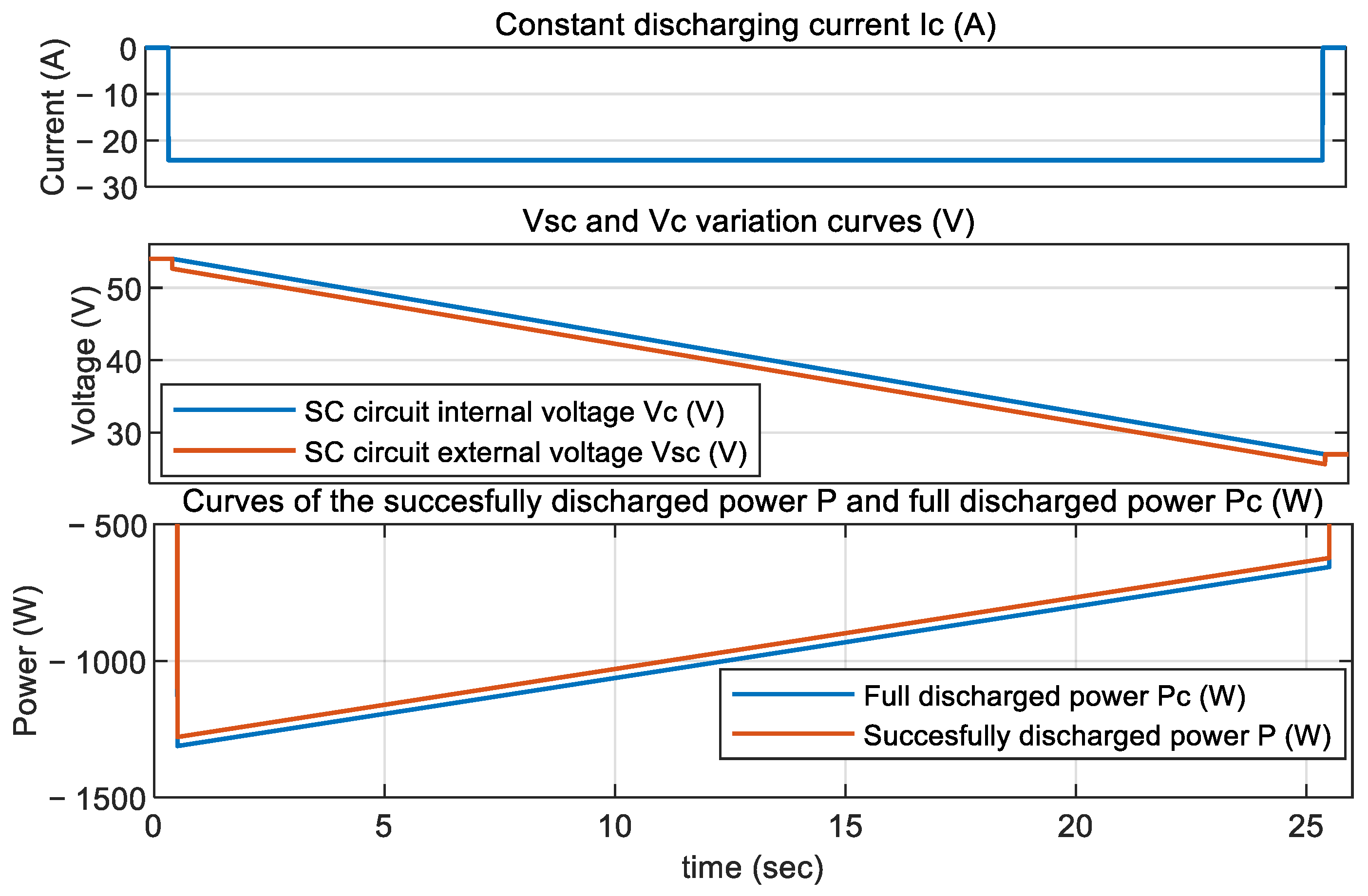
From simulation result graphs in Figure 2, it is visible how, at constant charging current, the internal voltage V_C increases linearly. Since the voltage V_R is constant all the time, the external voltage V_SC is higher than V_C by the same value all the time during charging. The total charging power p, which is the sum of successfully stored power p_C and lost power p_R, increases linearly during the charging time and is always higher by the same value than p_C.

To calculate the efficiency of the charging process, it is necessary to know both the energy successfully stored and the total energy delivered during charging. If an SC circuit with capacitance C is charged from an initial voltage V_C1 to a final voltage V_C2 in time t, then the stored energy E_C can be calculated using the expression:

$$E_C=\frac{C\left(V_{C2}^2-V_{C1}^2\right)}{2}.$$

(5)

Since the charging current I_C is constant all the time, the power lost due to the internal resistance R of the SC is also constant. Therefore, the energy that is lost during the whole charging process duration can be calculated by the formula:

$$E_R=I_C^{2}Rt.$$

(6)

The total energy E_SC fed to the SC circuit during the charging process consists of the stored energy E_C calculated by (5) and the lost energy E_R calculated by (6):

$$E_{SC}=E_C+E_R.$$

(7)

The full efficiency of the charging process is calculated as the energy stored in E_C divided by the total energy fed to the SC circuit:

$${\eta }_c=\frac{E_C}{E_{SC}}.$$

(8)

In the discharging process, unlike in the charging process, the initial voltage of the SC circuit is higher than the final voltage, so for discharging time duration t the constant discharging current is calculated by the same Equation (3), obtaining a current with the same numerical value as in the charging case but with minus sign indicating that the current flows in the opposite direction. SC circuit constant current discharge process simulation diagrams are shown in Figure 3 and, if the results are compared with those from Figure 2, it is visible that the charging and discharging processes are like mirror images.

The energy that is lost during the discharging process is calculated using the same Equation (6), while the energy E_S that successfully reaches the consumer is calculated as the difference between the total energy E_C, discharged from the SC circuit, and the lost energy E_R:

$$E_S=E_C-E_R.$$

(9)

The full efficiency of the discharging process is calculated as the energy E_S divided by the energy E_C:

$${\eta }_d=\frac{E_S}{E_C}.$$

(10)

The full efficiency of the charging/discharging process, when the charge from V_C1 to V_C2 and the following discharge from V_C2 to V_C1 occur at equal times, can be calculated as the energy E_S of Equation (9) divided by the energy E_SC of Equation (7):

$${\eta }_t=\frac{E_S}{E_{SC}}.$$

(11)

During the simulation, the curves of the instantaneous values of the energy charging and discharging efficiencies calculated by Equations (8) and (11) can be plotted as shown in Figure 4. It is also possible to obtain the instantaneous curve of the power storing efficiency, which can be calculated with the expression:

$${\eta }_{Pch}=\frac{P_c}{P_c+P_R}.$$

(12)

The instantaneous curve of power discharging efficiency in real time is obtained by:

$${\eta }_{Pdis}=\frac{P_c-P_R}{P_c}.$$

(13)

Although the main values of interest are the energy storage efficiency at the very end of the charging process and the energy discharge efficiency at the very end of the discharging process, Figure 4 shows visually how the power and energy storing and discharging efficiency changes during SC circuit charging and discharging, respectively. At the start of the charging process, power and energy storage efficiencies are at their lowest points but gradually increase thereafter. At the start of the discharging process, the power and energy discharge efficiencies are at their highest points but gradually decrease thereafter. It is visible that the full efficiency of the discharging process is slightly lower than the full efficiency of the charging process. The fact that the charging and discharging processes are not identical in terms of efficiency is because the total energy that is discharged during the discharging process corresponds to the energy that is successfully stored during the charging process, and some of this energy is lost during discharge due to the internal resistance R. In the case of charging, the lost energy is compensated by taking more energy from the source, thus ensuring that charging is completed after the scheduled time t. Mathematically, it can also be verified that the magnitude of this difference in efficiency depends on the internal resistance R.

4. Supercapacitor Charging and Discharging with Constant Input Power

In this charging case, the only constant parameter is the input power P, denoted by a capital letter in Figure 5. The other parameters, such as charging current I_C, voltage drop V_R, internal voltage V_C and external voltage V_SC are variables denoted by lower case letters.

Therefore, the constant total power fed to the SC is equal to the sum of the successfully stored power p_c and the lost power p_R:

$$P=p_c+p_R.$$

(14)

For the charging case, the corresponding power balance equation is:

$$P=v_c{i}_c+i_c^{2}R.$$

(15)

During charging, the relationship between the current i_c and the capacitance C is:

$$v_c^{\prime }\left(t\right)=\frac{i_c}{C}.$$

(16)

Using Equation (15) to transform Equation (16), the differential equation obtains:

$$R{C}^2{v}_c^{\prime }{\left(t\right)}^2+{Cv}_c{v}_c^{\prime }\left(t\right)-P=0.$$

(17)

Dividing Equation (17) by the capacitance C obtains:

$$RC{v}_c^{\prime }{\left(t\right)}^2+v_c{v}_c^{\prime }\left(t\right)-\frac{P}{C}=0$$

(18)

The solution of the quadratic Equation (18) is:

$$v_c^{\prime }\left(t\right)=\frac{-v_c\pm \sqrt{v_c^2+4RP}}{2RC}.$$

(19)

The correct version of Equation (19) is with a plus sign before the square root. This can be resolved by comparing Equation (19) with Equation (16), since the charging current must be positive. Next, the differential equation for calculating the charging time t can be derived from Equation (24):

$$dt=\frac{2RC}{-v_c+\sqrt{v_c^2+4RP}}d{v}_c$$

(20)

The formula for calculating the charging time t is derived by integrating Equation (20), if the voltage V_C changes from V_C1 to V_C2 over the time duration t under the condition that V_C1 < V_C2, resulting in the expression:

$$t=\frac{C}{4P}\left(V_{C2}^2-V_{C1}^2+V_{C2}·\sqrt{4RP+V_{C2}^2}-V_{C1}·\sqrt{4RP+V_{C1}^2}+4RP·\mathit{LN}\left(\frac{V_{C2}+\sqrt{4RP+V_{C2}^2}}{V_{C1}+\sqrt{4RP+V_{C1}^2}}\right)\right)$$

(21)

According to Equation (21), there is no problem in calculating the charging time t for a known constant power P, initial voltage V_C1 and final voltage V_C2. The formulation of the problem statement for the given situation would be how long it would take the SC circuit voltage to increase from V_C1 to V_C2 if a constant power P were applied to it. However, the next option of interest is to calculate the required power P fed to the SC circuit at a known charging time t, initial voltage V_C1 and final voltage V_C2. The formulation of the problem statement for the given situation would be as follows: what constant power P must be fed to the SC circuit to charge it from V_C1 to V_C2 during time duration t? Equation (21) is transcendental, so the formula for calculating the power P cannot be derived directly from it. Regarding the discharge case Equation (32) that is rather similar to Equation (21), reference [30] describes how other parameters, such as current i_C voltages v_C, v_R, etc., can be calculated in real time using the Lambert W function, but not the constant P depending on specified time t. One option for solving the power P is to use a mathematical computation program such as Wolfram since, by inputting Equation (21) with corresponding values of the known parameters, the numerical value of power P is solved. The second option is to make a table of the results of solving Equation (21) at different powers P, because then the corresponding power P can be found for the planned charging time t. For example, an array of charging times t can be formed where the power P varies from 750 W to 9000 W in steps of 0.1 W. At these values of P, charging takes place from approximately 33.6 s to 3.6 s, and Figure 5 shows the time curve versus the constant power P supplied to the SC circuit.

Both in the table of P and t arrays and in the t diagram of Figure 6, it is possible to find the specific charging time t of interest and then read the corresponding power P. For a given power step change of 0.1 W, there is also some small error in the solution. To reduce this error, the step change in P should be reduced even further, bringing the results closer to absolute accuracy. For example, looking for the power P at time t = 25 s, the actual value of the charging time found is approx. 25.0012 s as shown in Figure 7, and the power P = 1018.3 W corresponding to this time value is also selected. However, the error in this case is very low, being only a thousandth of a second.

Since the Equation (21) contains sub-root expressions, there is a limited range of valid values of power P, which can be determined by writing a system of inequalities:

$$\left\{\begin{array}{c}4RP+V_{C2}^2\ge 0\\ 4RP+V_{C1}^2\ge 0\end{array}\right.$$

(22)

Solving the Equation (22), the range of definition of the power P values becomes:

$$P\ge -\frac{V_{C1}^2}{4R}.$$

(23)

There is no purely mathematical limit to positive values of P, but there is a limit up to a certain negative value of the power P. However, in the case of charging, this is apparently not the case, as a negative fed power would already mean a discharge. In the case of discharge, which will be described further, the ranges of definition of the sub-root expressions will be more relevant. The example in Figure 7 shows the simulation results of charging the SC circuit for 25 s with the predetermined constant power P = 1018.3 W.

Since a constant power P is fed to the SC circuit during the entire charging time t, the total energy fed to the SC circuit is calculated as the product of power P and time t:

$$E_{SC}=Pt.$$

(24)

The stored energy E_C is known in advance, as it is calculated using the same Equation (5). Therefore, the lost energy E_R is calculated as the difference between E_SC and E_C, while the full efficiency of the charging process is calculated using the same Equation (8). The efficiency of real-time power storage is calculated using the same Equation (12).

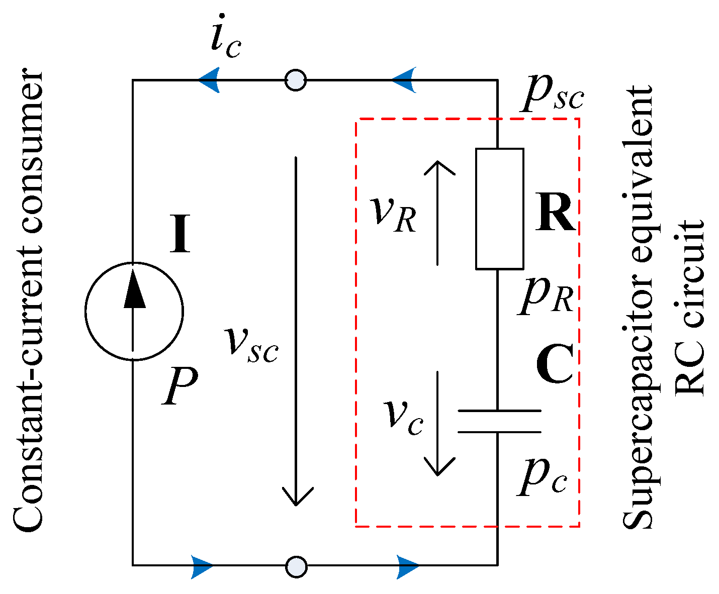
In the case of SC discharging, a consumer connected to the SC circuit is assumed to consume a constant power P, as shown in Figure 8, where this consumer is equivalently replaced by a current source. Variable parameters in lower case letters are the same as those in the SC charging case earlier.

As a result, the constant power consumption P corresponds to the difference between the total discharged power p_c and the lost power p_R:

$$P=p_c-p_R.$$

(25)

For the discharging case, the corresponding power balance equation is:

$$P=v_c{i}_c-i_c^{2}R.$$

(26)

During the discharging process, there is the following relationship between the current i_c and the capacitance C:

$$v_c^{\prime }\left(t\right)=-\frac{i_c}{C}.$$

(27)

Using Equation (27) to transform Equation (26), the following differential equation can be obtained:

$$R{C}^2{v}_c^{\prime }{\left(t\right)}^2+{Cv}_c{v}_c^{\prime }\left(t\right)+P=0.$$

(28)

Dividing Equation (28) by the capacitance RC² obtains:

$$v_c^{\prime }{\left(t\right)}^2+\frac{v_c}{RC}{v}_c^{\prime }\left(t\right)+\frac{P}{R{C}^2}=0.$$

(29)

The solution of the quadratic Equation (29) is:

$$v_c^{\prime }\left(t\right)=\frac{-v_c\pm \sqrt{v_c^2-4PR}}{2RC}.$$

(30)

The correct version of Equation (30) is with a plus sign before the square root. This can be resolved by comparing Equation (30) with Equation (27), as the discharge current should be as low as possible to increase efficiency. Next, the differential equation for calculating the discharging time t can be derived from Equation (30):

$$dt=\frac{2RC}{-v_c+\sqrt{v_c^2-4PR}}d{v}_c.$$

(31)

The formula for calculating the discharging time t is derived by integrating the Equation (36), if the voltage V_C changes from V_C2 to V_C1 over the time duration t under the condition that V_C2 > V_C1, resulting in the expression [30,32]:

$$t=\frac{C}{4P}\left(V_{C2}^2-V_{C1}^2+V_{C2}·\sqrt{V_{C2}^2-4PR}-V_{C1}·\sqrt{V_{C1}^2-4PR}-4PR·\mathit{LN}\left(\frac{V_{C2}+\sqrt{V_{C2}^2-4PR}}{V_{C1}+\sqrt{V_{C1}^2-4PR}}\right)\right)$$

(32)

It should be noted that, even though there is a discharge, the Equation (32) assumes that the power P is positive. The formulation of the problem statement for the given situation would be how long it would take the SC circuit voltage to decrease from V_C2 to V_C1 if a consumer, connected to this SC circuit, consumes a constant power P. However, the next option of interest is to calculate the constant power P that must be consumed by a consumer to decrease the SC circuit voltage from V_C2 to V_C1 during time duration t. As with Equation (21), the same conclusions can be drawn that the formula for calculating the power P cannot be derived directly from Equation (32), so the same two options exist with the use of a mathematical computing program or the use of a pre-calculated table of time t and P values.

In the case of constant charging/discharging current, it is a fact that, after charging the SC circuit with a certain current at time duration t from the initial voltage V_C1 to the final voltage V_C2, it can then be discharged with the same current at the same duration t from voltage V_C2 to V_C1, as shown in Figure 2 and Figure 3. On the contrary, the SC circuit cannot be discharged from V_C2 to V_C1 in time t at the same power as it was previously charged. It was clarified that, in the case of constant charging/discharging power, only one of the parameters—time t or power P—can be equal to the corresponding parameter from the charging process.

If the discharging process is planned to last the same duration t as the charging process, then the consumer’s constant power is lower than the constant power stored during the charging process. On the other hand, if the discharging process is planned to occur at the same constant power as the charging process, then the discharge is faster. Figure 9 shows the comparative curves of the charging/discharging times versus a constant charging/discharging power, and it is visible that the difference between the charging and discharging times increases with increasing power value and decreasing comparative charging/discharging time. The green curve in Figure 9 becomes a red dashed curve at one point (325.4 W) meaning that, at further powers of P in Equation (32) the values of the sub-root expression with V_C2 emerge as negative, so the red dashed curve corresponds to the real parts of the complex numbers in the results for Equation (32), but in general this is an undefined region of power P values at given discharge conditions.

For testing reasons, the computer model can be set to one of the red line discharge powers and, if the simulation is run, it will simulate a discharge for a while, but at some moment the simulation will stop with an error message. Thus, from Equation (32), the range of valid values of the maximum constant discharging power can be determined by first writing the following system of inequalities:

$$\left\{\begin{array}{c}{V}_{C2}^2-4RP\ge 0\\ V_{C1}^2-4RP\ge 0\end{array}\right.$$

(33)

Solving Equation (33), the range of definition of power P values becomes:

$$P\le \frac{V_{C1}^2}{4R}.$$

(34)

The point with the green curve ending and the red dashed curve beginning corresponds to the result of Equation (34) in the case with an equal sign. Although the red-dashed curve in Figure 9, which is the real part of the complex results of Equation (32), looks like a symmetrical continuation of the green curve, in fact it is not possible to discharge the SC circuit to the required voltage of 27 V with these red-zone powers.

Simulation of the SC circuit discharging at a constant power of 4000 W for 5 s was tried and Figure 10 shows that discharging occurs for a while, but the simulation hangs when the V_C is discharged to approx. 30 V. Before the simulation stops, the current i_c and the total discharged power p_c start to increase rapidly while the voltage v_c starts to decrease rapidly, and therefore it can be concluded that at such low voltages the SC circuit is no longer able to provide the increasing total discharge power p_c that is necessary to provide the 4000 W required constant power P, so the simulation hangs. In a real situation, the consumer’s power would no longer be constant and would start to decrease according to the SC’s capability.

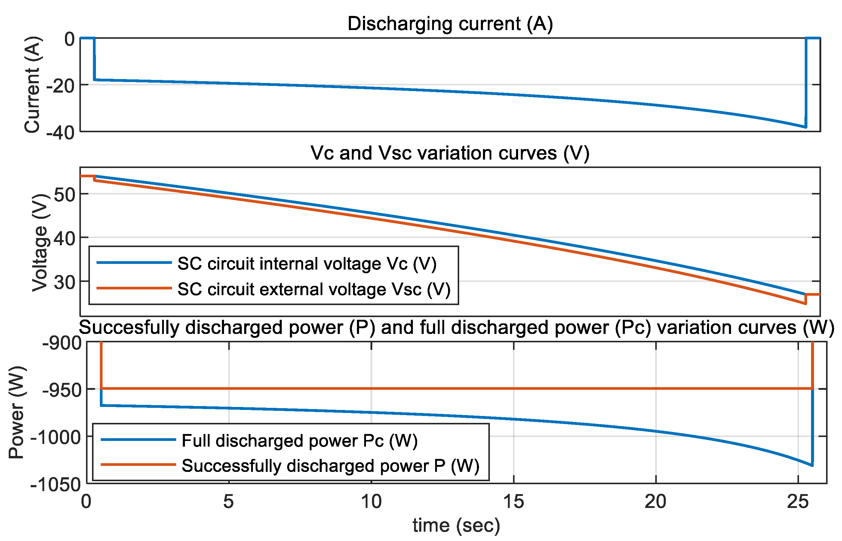
Figure 11 shows the simulation results of discharging the SC circuit for 25 s from V_C1 = 54 V to V_C2 = 27 V with constant successfully consumed power P = 949.5 W.

Since, during the discharge process the SC circuit feeds a consumer with a constant power P, which is considered as successfully discharged power, the successfully discharged energy can be calculated as the product of the power P and the time t:

$$E_s=Pt.$$

(35)

The total discharged energy E_C is known and is calculated by Equation (5), so the efficiency of the discharging process can be calculated by Equation (10). The full efficiency of the charging/discharging process is calculated using Equation (11). The power discharging efficiency is calculated using the same Equation (13). Figure 12 shows the real-time variation of power and energy storing/discharging efficiency.

5. Efficiency Comparison of Constant-Current and Constant-Power Charging/Discharging Strategies

Further, the efficiencies for constant current charging and constant power charging, the efficiencies for constant current discharging and constant power discharging, and the full charging/discharging cycle efficiencies of these two methods will be compared in detail. The corresponding calculations will be made for the same SC circuit under the same conditions, assuming that it is charged from 27 V to 54 V and then discharged back to 27 V for the same time duration as charging. According to the manufacturer’s information, the recommended maximum short-time peak current of the SC element in question is 240 A. Therefore, the cases of 1 s, 2 s and 3 s charging/discharging will not be considered in order to keep the charging discharging current below 200 A for efficiency improvement, since, according to Equation (4), the constant charging/discharging currents at these durations are above 200 A. Charges of 4 s to 30 s and discharges of the same durations with a change step of 1 s will be considered. Figure 13 shows the curve of charging/discharging current values, calculated by Equation (4), as a function of equal charging and discharging durations.

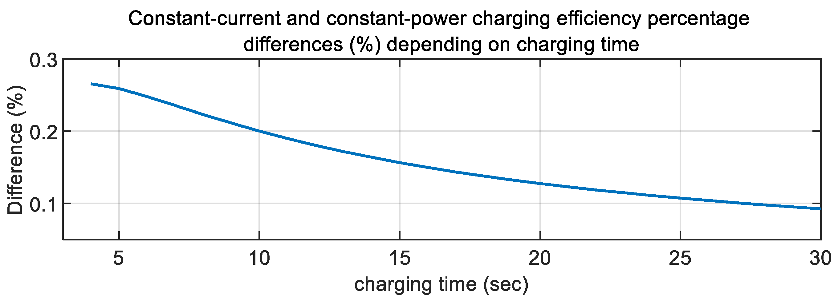
Although not very significantly, the results in Figure 14 show that charging with constant current is more efficient than charging with constant input power, and Figure 15 shows the percentage differences, which range from approx. 0.1 to 0.25%. This percentage difference is larger for faster charges and lower for longer charges.

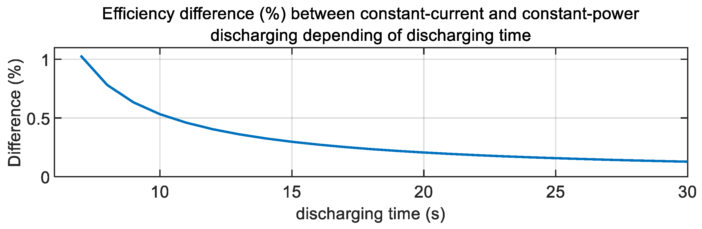
The initial discharging time with the constant consumer’s power is 7 s, because in Equation (32) the sub-root expressions with V_C2 come out negative for charging times that are less than 7 s, so they do not have valid power, as described before with reference to Figure 9. As visible in Figure 16 and Figure 17, the constant current discharging case is noticeably more efficient compared to the charging case from Figure 14 and Figure 15.

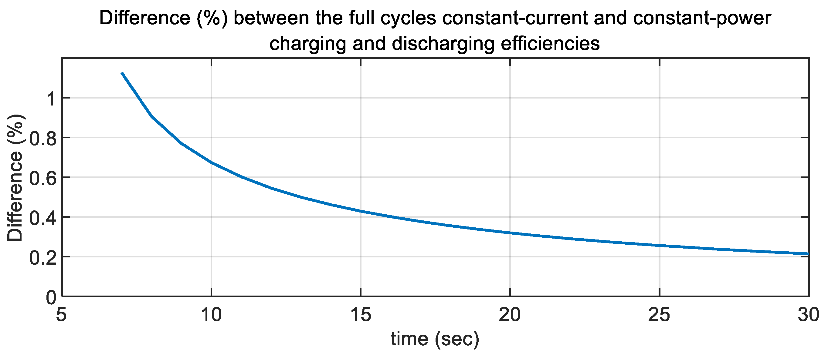
Figure 18 shows how the charging/discharging efficiency of constant current is higher than the charging/discharging efficiency of constant power charging/discharging and Figure 19 shows the exact numerical differences. At faster charges this difference is higher and at longer charges the difference gradually decreases.

The described charging efficiencies of constant current and constant power vary during charging time. For example, Figure 20 shows a comparison of the power storing efficiencies at the previously simulated charges for an SC circuit from 27 V to 54 V over 25 s. The variant with constant current charging has a higher efficiency at the start of charging while the efficiency of constant consumer’s power variant increases more quickly until it exceeds the efficiency of constant current charging at a certain point.

Looking at Figure 21, constant-current charging has a higher energy storing efficiency throughout the charging period. Although the energy storing efficiency of constant charging power increases quite rapidly and at the end of charging almost approaches the efficiency of the constant current variant, the latter still has higher total efficiency, shown in the last point of the graph.

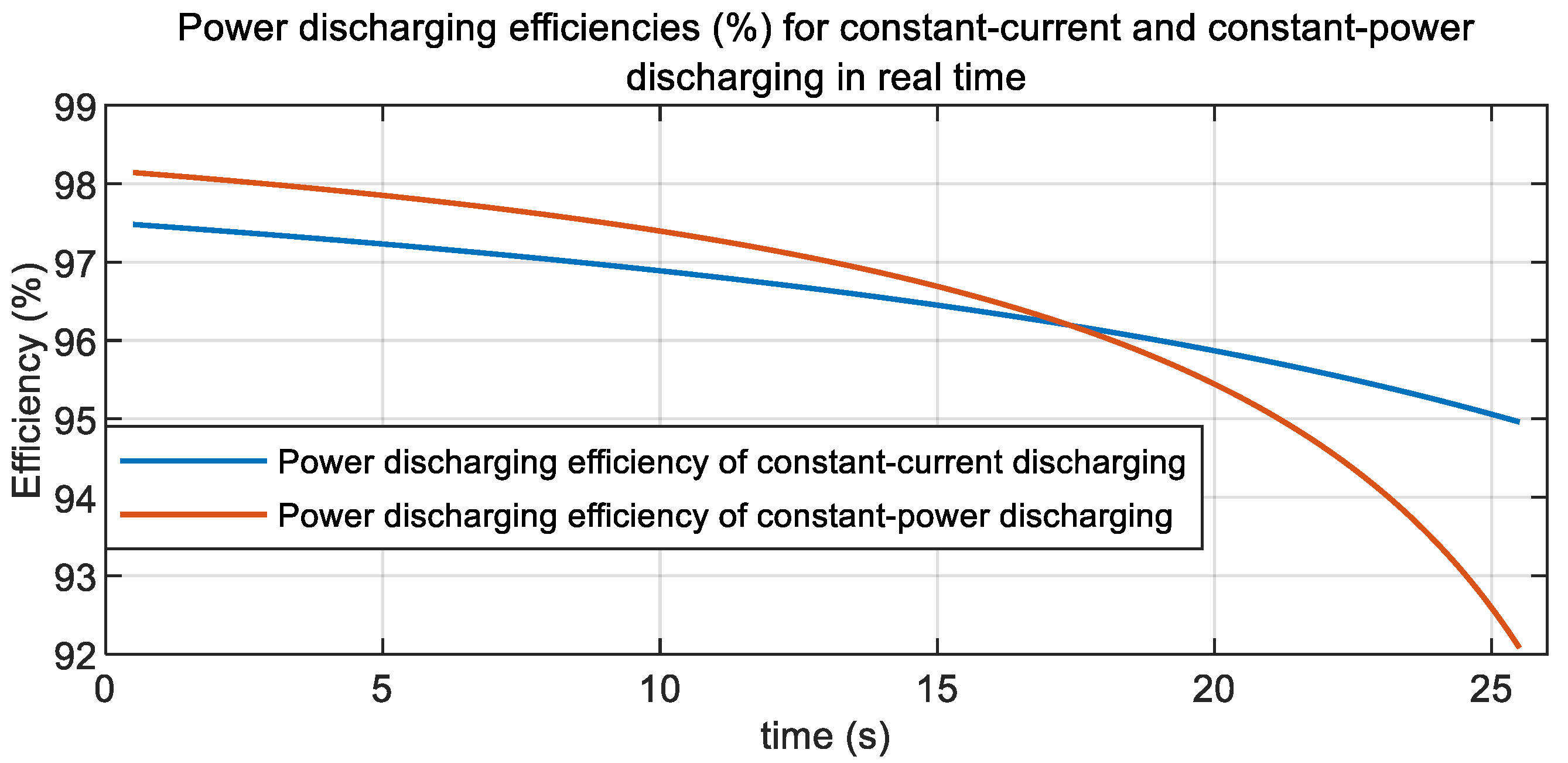
Figure 22 shows a comparison of the power discharge efficiencies when discharging from 54 V back to 27 V in 25 s. Although, at the beginning of the discharge, the efficiency of the constant-power discharge variant is higher than that of the constant-current discharge variant, its efficiency decreases more rapidly over time until it falls below the efficiency of the constant-current discharging.

Looking also at Figure 23, at the beginning of the discharge the efficiency of the constant power variant is higher, but at the very end it becomes lower.

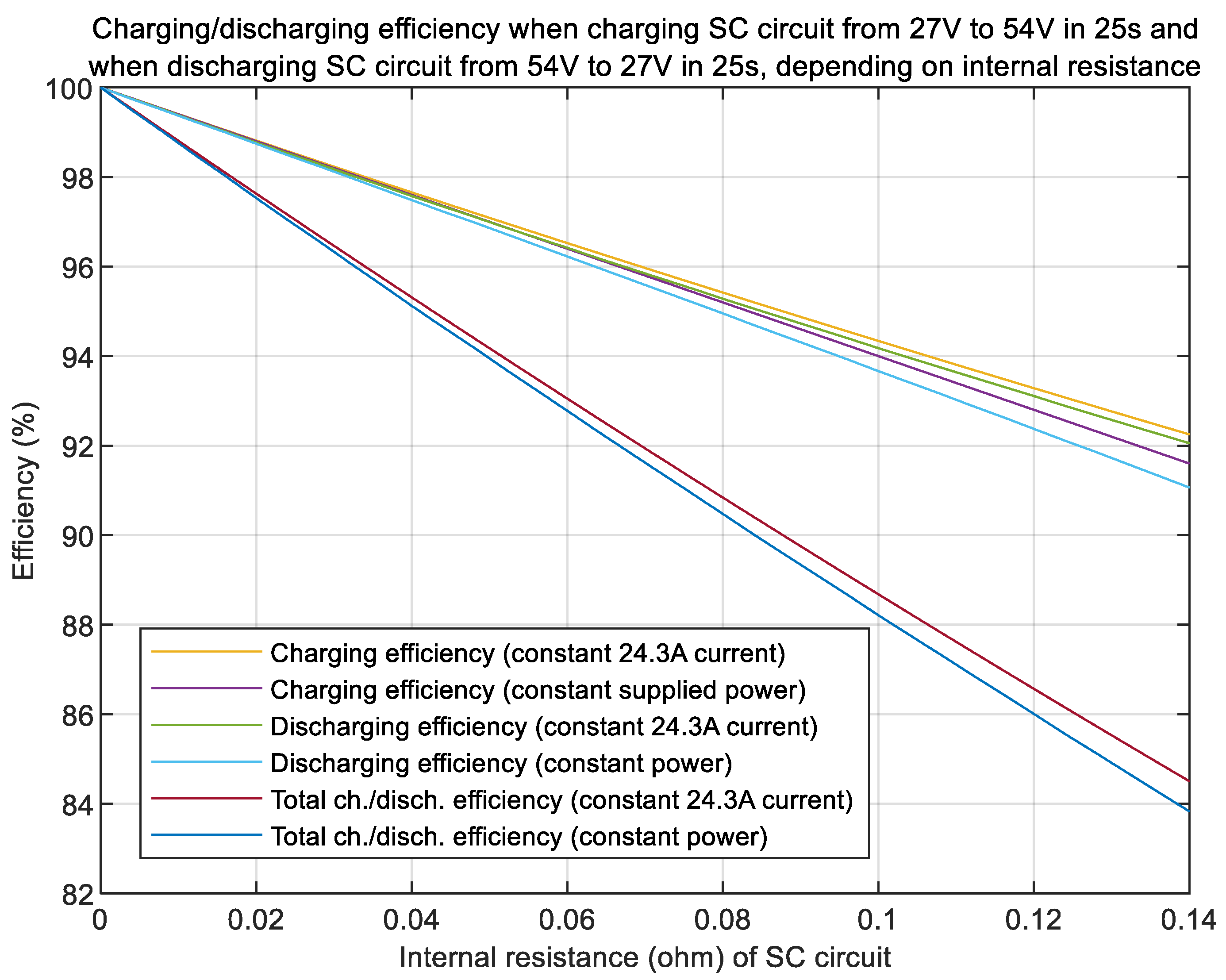
After finding that charging the SC circuit with a constant current is more efficient than charging with a constant supplied power, and that discharging the SC circuit with a constant current is more efficient than discharging with a constant power, it was decided to test how this difference varies with the internal resistance R of the SC circuit. In the calculations and simulations carried out so far, the internal resistance R was 0.056 Ω, corresponding to the 20-cell series circuit under consideration, according to the information provided by the manufacturer, but now a comparison of the differences in efficiencies will be made when charging the same SC circuit from 27 V to 54 V for the same 25 s at different internal resistance R, varying from 0 Ω to 0.14 Ω in changing steps of 0.004 Ω. Manufacturers provide the information in the datasheets of SC cells that they have a lifetime of approximately one million charge/discharge cycles, during which the capacitance decreases by 20–25% and the internal resistance R increases by 100% of the initial one. Besides, high operating temperatures caused by rapid charge/discharge cycles can significantly accelerate their deterioration but, in further comparisons, the capacitance of a single SC cell will remain the same C = 22.5 F. In the case of constant-current charging/discharging, the corresponding current is the same 24.3 A for all resistances R from the mentioned range. For constant-power charging, the corresponding power at each R is found separately with the help of Equation (21) and results in 948.15 W to 1069.1 W. For constant-power discharging, the corresponding power at each R is found separately with the help of Equation (32) and results in 948.15 W to 896.2 W. According to the results of the further calculations, both charging and discharging with constant current are more efficient in any case, except when no internal resistance is assumed, i.e., R = 0, because in this case both strategies have equal 100% efficiency for both charging and discharging. In practice the case of zero internal resistance is impossible, because any SC will have some internal resistance. It can be logically concluded that the findings on higher efficiency of constant-current charging/discharging are true for any SC cell model with known C and R, and not only for the particular SC cell model considered in this work.

Figure 24 shows that, at lower internal resistances the difference between constant-current and constant-power charging is lower, while at higher internal resistances this difference gradually increases, and the same is visible for discharging. It is visible that the differences are more significant in the case of discharging than charging and Figure 25 shows the exact percentage numerical values. The most obvious differences are visible when comparing the efficiency of the full charging/discharging cycles.

Looking at the numerical differences in efficiency shown in Figure 25, it can be concluded that constant-current charging and discharging is only marginally more efficient than constant-power charging/discharging because the differences are significantly below 1%. That is why, from a practical point of view, both charging/discharging methods can be considered relatively equivalent in terms of efficiency. The calculations and results obtained confirm that, in terms of efficiency, both mathematically and physically, charging a capacitor with constant current is not identical to charging it with a constant power supplied to its input, just as discharging a capacitor with a constant current is not identical to discharging it with a constant power.

6. Experimental Charging/Discharging of Supercapacitors and Comparison of Measurement Results with Simulation Results

In the previous chapters, the simulations and calculations were based on an RC circuit model equivalent, which is simplified but often used in the design of SC energy storage systems, as in terms of precision its results do not differ much from more accurate and complex SC models. Nevertheless, it was decided to perform a constant-current charging and discharging of a real SC circuit, as well as a constant-power charging and discharging, to check if it is easy to verify the previously described theoretical calculations and their results, considering that the difference in efficiencies was found to be lower than 1%.

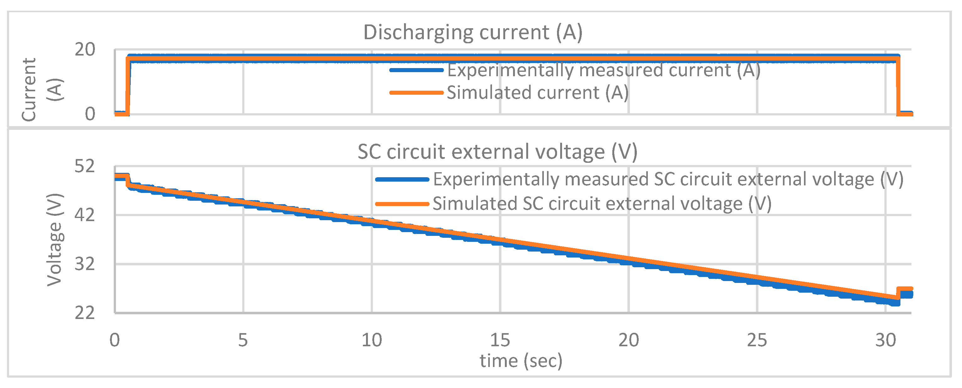
The same 20-cell SC series circuit will be charged using a power supply source that can supply either constant current or constant power, and discharged using an electronic load that can consume either constant power or constant current. Due to the maximum operating current of the available electronic load being 30 A, the charging/discharging conditions will be different: the initial minimum voltage of the circuit will be V_C1 = 27 V and the final maximum voltage will be V_C2 = 50 V, while charging and discharging times will be 30 s each. The experimental measurements were compared with the simulation results and the corresponding 20-cell circuit is shown in Figure 26. The electronic load EA-ELR 91500-30 was used in discharging mode, while the DC power supply EA-PSI 9550-60 was used in charging mode to provide load. Experimental waveforms were obtained using a Yokogawa DLM6054 oscilloscope and TA018 current probe.

In previous calculations and simulations of an RC circuit for the methods described, the determination of the parameter R should not rely only on the total internal resistance of SCs, but the conductive traces of the board can also have significant resistance, which in this case was found to be 46 mΩ using a micrometer. The resistance of the wires connecting the SC circuit to the power supply source in case of charging and to the electronic load in case of discharging is 6.3 mΩ. Both additional resistances were added to the internal resistance, so the total resistance to be used in the equivalent RC circuit for further calculations and simulations is R = 108.3 mΩ. The calculation of the constant charging/discharging current is not affected by R since it is calculated by Equation (4) and is I_C = 17.25 A. For constant-power charging, using the new R in Equation (21) and obtaining the corresponding curves as in Figure 6 and Figure 9, the corresponding power at 30 s is found to be 697.1 W. Accordingly, with constant-power discharging, using the new R in Equation (32), the corresponding power at the 30 s is found to be 630.6 W.

Figure 27, Figure 28, Figure 29 and Figure 30 show the results of the experimental measurements together with the simulation results in the same planes, and the oscilloscope measurements have some signal fluctuations due to electronic load switching actions, which make the curves not as smooth as in the simulations.

The experimental results show that, when discharging with both constant current and constant power, the discharge is still a little faster, as the final voltage after 30 s is slightly lower than the simulated and planned 27 V, but the differences are insignificantly small. A similar conclusion can also be drawn for experimental charges where the voltages after 30 s are slightly above the planned and simulated 50 V. Nevertheless, these statements are based on the visual differences between the expected results and the actual measured results shown by the graphs. In order to gain a more precise view of the accuracy of the measurements, the root-mean-square error (RMSE) method was used over a 30 s period, which in Figure 27, Figure 28, Figure 29 and Figure 30 ranges from 0.5th to 30.5th second. The corresponding formula for calculating the root mean square for either SC current or SC external voltage is:

$$RMSE=\sqrt{\frac{\sum _{i=1}^n{\left(x_i-y_i\right)}^2}{n}}$$

(36)

In Equation (36), x_i is the expected measurement result, y_i is the actual measured result and n = 75,000 is the number of measurements taken within 30 s. In each case for Figure 27, Figure 28, Figure 29 and Figure 30, the RMSE of both SC current and SC external voltage was calculated with Equation (36) and the results are shown in

Table 1. SC current and external voltage RMSE values of charging and discharging processes.

Measurement	Constant-Current Discharging	Constant-Current Charging	Constant-Power Discharging	Constant-Power Charging
SC current RMSE (A)	0.58	1.28	0.72	1.18
SC external voltage RMSE (V)	0.62	0.91	0.8	0.72

.

The smaller and closer to zero the RMSE is, the more accurately the measurements match the expected results, but slight numerical deviations can be seen in Table 1 above. In each case, one of the reasons for this inaccuracy might be the use of a simplified RC model for theoretical calculations and simulations. The second reason for the differences is that the exact capacitance of the SC circuit might differ by some amount from the calculated one because the capacitance of the capacitors decreases with time. Capacitance reduction can be relevant for both constant-current and constant-power charging/discharging, where the capacitance value is used to calculate the respective charging/discharging current and the respective charging/discharging power. The third reason is that the total internal resistance of the SC circuit might differ by some amount from the calculated one, because internal resistance of capacitors increases with time.

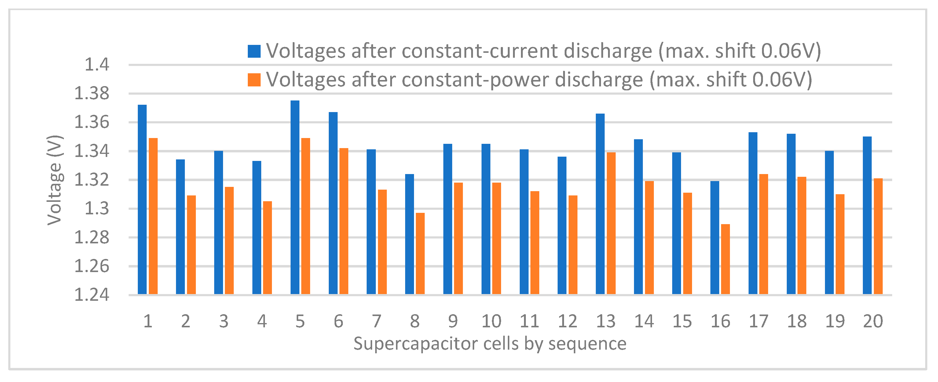
Moreover, the capacitance and internal resistance of individual SCs may also have changed unevenly over time, as voltage balancing circuits do not always work ideally enough to ensure equal voltages on each cell. Therefore, both before and after the charges and discharges, the voltages on each individual SC cell were also measured with a voltmeter to check how evenly the total circuit voltage was distributed across the individual SCs, and some shifts were also detected as a result. As visible in Figure 31 and Figure 32, there is a sort of symmetry in the voltage shifts after every four following SC cells. Different balancing plates might have different characteristics, but in the given situation the maximum differences between two separate SC cells are between 0.04 V and 0.06 V.

Using the RMSE method, the average errors of the voltage values on an individual SC cell were calculated for each of the cases shown in Figure 31 and Figure 32, assuming that the entire SC circuit voltage is the sum of the measured individual cell voltages, while the voltage of a single cell should be the circuit voltage divided by the number of cells.

Table 2. SC single cell voltage RMSE values in different cases.

Case	RMSE Value (V)
RMSE before the first discharge	0.012
RMSE after constant-current discharge	0.015
RMSE after constant-current charge	0.015
RMSE after constant-power discharge	0.015
RMSE after constant-power charge	0.016

shows the corresponding results, and it is visible that the voltage deviations are not high.

Comparing experimental and simulation results, it can be concluded that constant-current and constant-power charging/discharging methods are nearly similar in terms of charging/discharging SC circuit in the planned time, but there are still some inaccuracies due to the reasons mentioned. Therefore, such practical experiments produce results that are approximately identical to the simulation results. Hence, it is very difficult to clearly verify in a practical way the previously gained conclusion that constant-current charging/discharging is more efficient than constant-power charging/discharging, especially if the difference is less than 1%.

7. Discussion

The basic methods to charge capacitors are constant-current charging and constant-power charging. Similarly, capacitors can be discharged at constant current and constant power, understanding that in the former case the consumer connected to the capacitor consumes a constant current and in the latter case it consumes constant power. Initially, it may be thought that the two charging methods—constant-current and constant-power charging—should be identical in terms of efficiency, while also the two discharging methods—constant-current and constant-power discharging—should be identical in terms of efficiency, in cases where each method charges an SC circuit from a certain initial voltage to a certain final voltage within a specified time and then discharges it to the previous voltage during the same time duration. Detailed comparisons confirmed that, in any case, constant-current charging/discharging is more efficient than constant-power charging/discharging under the same boundary conditions when a supercapacitor equivalent replacement RC model is used, as the basis for the calculations. However, these differences in efficiency, which vary also with the internal resistance R of the capacitors, are significantly lower than 1% for the cases considered in this work. To gain this finding, it is necessary to choose a certain supercapacitor cell with known R and C to perform the corresponding calculations. In fact, apart from the particular supercapacitor cell considered in this work, the finding is true for any supercapacitor cell with known R and C, since the same calculating formulas could be used. Different supercapacitor cells with their R and C might differ in the amount by which constant-current charging/discharging is more efficient than constant-power charging discharging and this can be calculated by the equations derived in this paper.

Since the differences in efficiencies of the two methods are so small, both can be considered nearly equal from a practical point of view in certain applications, but in some applications even such a small difference can be substantial. The main novelty of this work is the finding and fundamental justification that, in an RC circuit, charging a capacitor with constant current is not completely identical in terms of efficiency to charging it with constant power under the same boundary conditions. The same conclusion can be drawn for discharging a capacitor with constant current and discharging it with constant power. The two methods are identical in terms of efficiency only if the internal resistance R of the capacitors equals zero, but this is not possible in a real circuit.

Precise experimental validation of the findings on the differences in charge/discharge methods on a real supercapacitor circuit is difficult, as a real supercapacitor slightly differs from a simplified RC circuit for several electrical, thermal and chemical reasons and precise R and C are not known. Nevertheless, the simplified RC model is the most commonly used model globally for the planning of supercapacitor energy storage systems, since, according to previous studies, the operation of the simplified RC circuit differs by slightly above 5% from the operation of more complex models closer to the real supercapacitor. This inaccuracy is small enough for the RC model to be used in the designing of large-scale supercapacitor systems, but too high for a real supercapacitor circuit to validate the theoretical findings from an idealized RC circuit described in this work.

Despite of small differences, the finding that constant-current charging is more efficient than constant-power charging could be seen as more significant from a practical point of view, in the sense that such simple constant-current or constant-power SC charging occurs more frequently than constant-current or constant-power discharging. For example, when charging SC from a microgrid or solar panels, it might be worth preferring constant-current charging. In case of regenerated energy storage in the SC system of an electric vehicle, both the charging current and power are usually variable, but it is possible to set a maximum charging current for the SC system, meaning that the SC charges at constant current and the remaining regenerated energy is dissipated in braking resistors. As for the discharge case, consumers, such as electric vehicles, for example, most often consume variable power and current. SC discharging strategies often discharge SCs in proportion to the power demand of the electric transport. Nevertheless, it is also possible to set the SC to supply the vehicle with a certain constant current or a certain constant power while the vehicle is moving, and the remaining part is taken from the grid.

As constant-current charging/discharging is more efficient than constant-power charging/discharging under the same boundary conditions, it means that the second case has more wasted energy, causing the SCs to heat up more, thus contributing to their ageing. On the one hand, due to the difference in efficiencies below 1%, it can be assumed that, for episodic charging/discharging, the SCs wear out similarly in both methods. However, looking at the long term over the whole service life of the SC cell, it follows that this difference might slow down the ageing of the SC cell if such charge/discharge cycles with constant current are to be performed continuously. Therefore, if an SC cell is charged/discharged many times at a constant current rather than at a constant power, then it will serve longer by the amount by which the efficiency of the constant current method is higher than that of the constant power.