Influence of Atmospheric Stability on Wind Turbine Energy Production: A Case Study of the Coastal Region of Yucatan

Abstract

Wind energy production mainly depends on atmospheric conditions. The atmospheric stability can be described through different parameters, such as wind shear, turbulence intensity, bulk Richardson number, and the Monin–Obukhov length. Although they are frequently used in micrometeorology and the wind industry, there is no standard comparison method. This study describes the atmospheric stability of a coastal region of Yucatan, Mexico, using these four parameters. They are calculated using six-month data from a meteorological mast and a marine buoy to determine atmospheric stability conditions and compare their results. The unstable atmospheric condition was predominant at the site, with an 80% occurrence during the measurement period, followed by 12% in neutral and 6% in stable conditions. Wind speed estimations were performed for each atmospheric stability scenario, and the variation in the energy produced was derived for each case. Unstable atmospheric conditions deliver up to 8% more power than stable conditions, while neutral conditions deliver up to 9% more energy than stable conditions. Therefore, considering a neutral state may lead to a considerably biased energy production estimation. Finally, an example calculation indicates that atmospheric stability is a crucial parameter in estimating wind energy production more accurately.

1. Introduction

Primary challenges related to sustainable development, namely, energy security, climate change, and access to energy, make a compelling case for using renewables on a large scale. World energy demand in 2020 fell by 4.5%. In addition, there was a collapse in demand for oil and gas, generating declines of 9.3% and 7% [1], respectively. Despite this abnormal behavior, the penetration of renewable energies in the energy market continued, and there were no setbacks. Moreover, renewable energies were the only source of electricity that maintained constant growth. In 2020, solar and wind energy increased 238 GW of installed power capacity, representing the most significant increase [1]. The growth of these two energy sources has been rapid, substantial, and continuous. This growth represented almost 10% of the total installed capacity, 2839 GW, at the end of the year. In this way, renewable energy (RE) sources represent approximately 29% of the world’s total final energy consumption.

This increase is expected to continue due to RE’s competitiveness compared to conventional generation sources in terms of decreasing operating costs. Over the past ten years, the average levelized cost of utility-scale solar PV decreased by 85%, while onshore wind costs decreased by 56%, leaving the levelized cost of electricity at 0.05 USD/kWh for solar PV and 0.039 USD/kWh for wind power [2]. This is due to the need for smart grids and decarbonization policies in many countries, prioritizing RE to mitigate climate change and reduce greenhouse gas emissions [3].

Despite all the mobility restrictions emanating from COVID-19, the wind energy market had one of its best years. The growth obtained during 2020 set a record since 93 GW was added to the installed capacity, representing an increase of 14%, reaching 743 GW [4], compared to 2019.

Wind power is a strong competitor to fossil fuel generation due to its rapid decrease in costs per kWh and its ability to supply a significant portion of electric demand, as it already does in several countries. Globally, operating wind power capacity represented approximately more than 6% of total electricity generation in 2020. For the 12th consecutive year, China led the top five countries with the highest increase in installed wind capacity, followed by the United States, Brazil, the Netherlands, and Spain. In Latin America, wind energy has become the fastest-growing RE source, with about 34 GW distributed in 26 countries in the region [3]. Despite Mexico’s regulatory policy changes in the last four years, the country added 0.6 MW to its installed capacity. Additionally, regions such as Baja California, Veracruz, Oaxaca, and Yucatan have attractive wind potential, and some have established large wind farms [5]. Specifically, the Yucatan Peninsula has a potential capacity of 6125 MW and an expected annual energy production of 14,802 GWh [6]. As of 2019, three wind farms have been operated in the region with an installed capacity of 244.7 MW [7,8,9].

Even though the installation of wind farms is becoming more frequent, there are essential factors to consider for their successful development. One of these factors is an adequate wind resource assessment to quantify the energy availability at a potential site. Wind speed is the most important factor since wind power depends on it. The best way to evaluate wind power is by analyzing meteorological measurements for each proposed turbine location. Unfortunately, this activity requires long-term measurement campaigns and substantial financial resources. For this reason, when wind data are unavailable, statistical analysis has been used to estimate wind speed values. The Weibull probability density function is the distribution widely used to describe wind speed statistics [10]. This information makes it possible to know some critical parameters, such as the maximum wind speed, the most probable wind speed, and the wind speed with the highest energy delivery, among others found on the site [11].

The parameters estimated by the Weibull distribution are essential to quantify the energy production of a wind turbine, which depends mainly on the wind speed frequency distribution [12]. On the other hand, the power generation of a wind turbine is influenced by the wind profile at hub height and turbulence intensity. High values of turbulence intensity decrease energy availability. Due to this, the most suitable sites for the exploitation of wind resources are those where the wind speed is high, and the level of turbulence intensity is moderate.

The amount of turbulence can be correlated with atmospheric stability, which is defined as the ability of the atmosphere to react to small disturbances (mitigating or promoting turbulence) in the vertical movements of an air parcel [13].

In terms of atmospheric stability, it is possible to have three primary states: stable, neutral, or unstable. In a stable atmosphere, there is a slight mixing between the layers of the atmosphere, producing a more significant vertical gradient of temperature and velocity. Limited mixing occurs in the neutral atmosphere, which keeps the vertical wind speed gradient constant. Finally, intense air mixing in an unstable atmosphere reduces velocity and temperature gradients in the vertical direction. Several parameters have been used to quantify atmospheric stability. These parameters include wind shear, turbulence intensity, gradient Richardson number, bulk Richardson number, Monin–Obukhov length, and turbulent kinetic energy [14].

According to the IEC standard [15], estimating the wind speed at different heights is possible using the Hellmann exponential or logarithmic profiles [12,16]. However, these models do not consider conditions that affect wind estimates, such as atmospheric stability, roughness, turbulence intensity, and shear. All these factors are characteristics of the atmospheric surface layer.

In these profiles, a neutral atmosphere is usually assumed, causing biases in wind speed forecasts that, in turn, affect energy production. Several studies have demonstrated that, when atmospheric stability is considered, there have been differences in power obtained through statistical analysis tools such as the Weibull distribution [17,18,19,20]. For example, at a particular wind speed, higher generation was obtained in stable conditions and lower in unstable conditions of high convection, with a difference of 15% in the average energy production of one wind turbine [21].

In his research study [22], St. Martin analyzed 2.5-month data, concluding that greater power was obtained at low speeds with high turbulence values than at lower turbulence conditions. The opposite happens for medium speeds (10–14 m/s); high turbulence leads to less power. When the power curves were analyzed with the parameters of turbulence intensity and Richardson number, statistically significant differences were found between them. However, there were not statistically significant differences in the power curves when analyzing other parameters such as turbulent kinetic energy, wind shear, or wind veer, possibly due to the stable conditions that prevail at the site. Finally, there was high annual energy production when atmospheric factors were not considered, leading to financial risks for operators and manufacturers.

Bardal [23] analyzed the effects of wind shear and turbulence in a wind turbine with data obtained from a LIDAR (light detection and ranging) station. They found differences of more than 1.2% in average annual energy production, which can lead to a significant bias in the economic revenue of a large wind farm.

In another study, the difference between annual energy production under unstable and neutral conditions was approximately 4% [24]. The authors also analyzed the impact of turbulence intensity $\left(TI\right)$, concluding that there can be differences of up to 3% between low and high $TI$.

Specifically, several studies have been carried out on the open sea to understand the effects of atmospheric stability on energy production. In [25], the authors concluded that wind speeds are overestimated since the height of the mixed atmospheric layer is also overestimated under neutral and unstable atmospheric conditions. Therefore, the authors developed a model to estimate the wind profile above sea level, considering atmospheric stability conditions.

On the other hand, Bahamonde [26] proposed a method to estimate the average speed at a certain height in open sea conditions, considering variations in atmospheric stability. After testing the method on a wind turbine, favorable results were obtained with slight deviations (1–2.5%) between measured and predicted results under unstable stratification.

Moreover, several studies have been carried out for coastal areas to determine atmospheric stability [27,28,29,30]. An additional research study aims to determine the impact that atmospheric conditions could have on the power extracted from the wind turbine. It was found that there is a lower performance during the day (−10%/−8%) and in unstable conditions (−11%/−3%), while during night hours (23%/23%) and in stable conditions (33%/37%), the yield is higher [31].

As can be seen from the literature review, there is evidence of a direct relationship between the atmospheric stability level and the number of periods of high energy production in wind farms. However, the above-mentioned studies are not conclusive about the effects of atmospheric conditions on energy production since, in some places, stable atmospheric regimes increase energy production. In contrast, other sites exhibit the same behavior when unstable conditions occur. Significant discrepancies between different methodologies to characterize atmospheric stability have been found. In all these studies, it was concluded that one of the main causes of variation in production is atmospheric stability. Therefore, models that accurately incorporate this aspect are necessary. This has increased interest in studying the stability conditions present at each site. For example, in the case of the Yucatan Peninsula, there are conditions that are not present in other places. Although the Yucatan Peninsula is located between the Gulf of Mexico and the Caribbean Sea, it has a low intensity of turbulence. This aspect gives the wind speed a steady characteristic, allowing it to generate moderate but continuous power [32,33,34]. Moreover, in these studies, parameters usually employed in micrometeorology are used to determine the site’s stability, and no comparisons are made with other parameters typically used in the wind industry. Therefore, there is no common framework for both areas—micrometeorology and the wind industry. In addition, they generally analyze only the impact on the wake area. For these reasons, the present research study raises the following questions:

• Is it possible that various atmospheric stability parameters converge?
• Is it necessary to adjust the intervals defined for these parameters depending on the site?
• How does atmospheric stability affect energy production?

Therefore, the differences that the atmospheric stability criterion can entail, and hence the need for robust methodologies that can include ensembles, are evaluated in this research study. In addition, even though micrometeorology and wind energy are related, there is no common analytical framework between them. Therefore, this study seeks to contribute to a framework that addresses these gaps. This study focuses on determining the atmospheric stability conditions of a coastal zone through various parameters used in micrometeorology and the wind industry, and their relationship with the variation in annual energy production. The authors propose a methodology according to the coastal region to determine four stability parameters; subsequently, a common framework for these parameters is presented; and finally, their influence on energy production is analyzed. Section 2 presents the study site, characteristics of the measurements, and parameters for the analysis of atmospheric stability. Section 3 presents the wind patterns of the site, as well as the diurnal behavior of stability parameters during the total measurement period. Section 4 presents the conclusions of the study.

2. Data and Methods

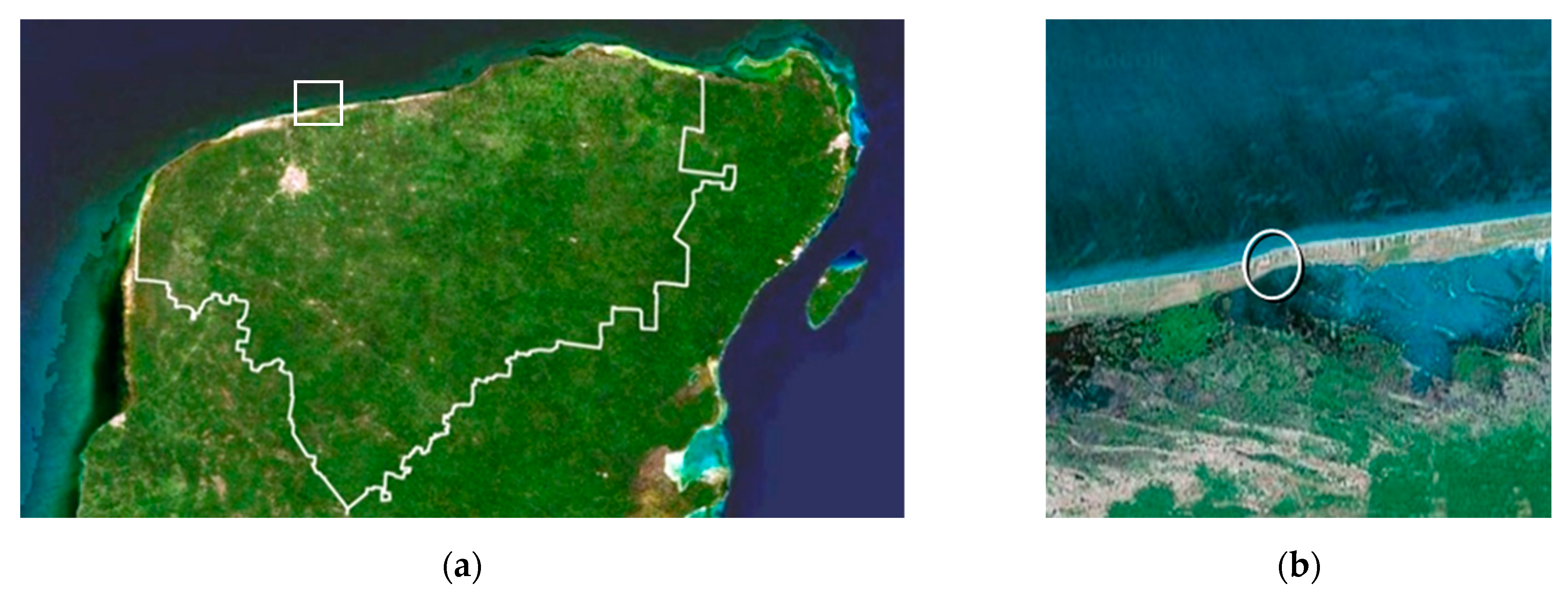
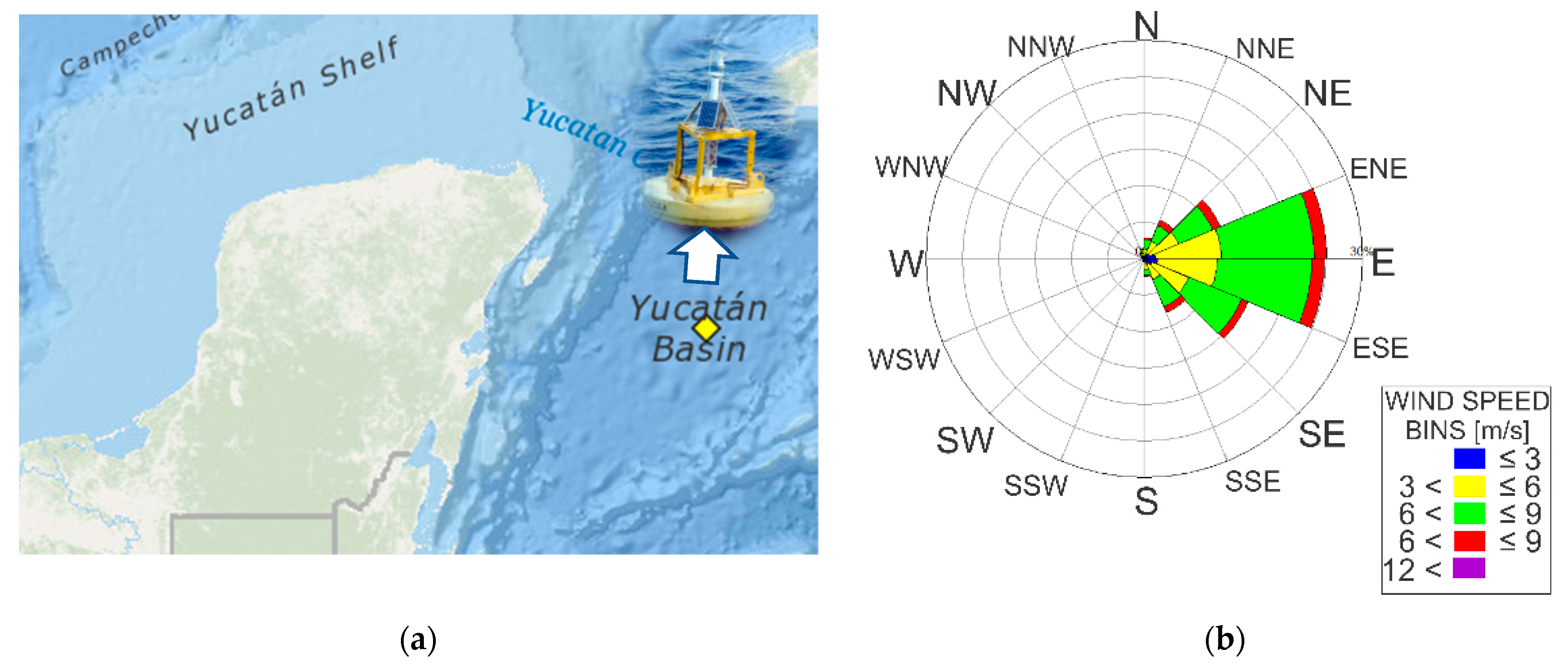
2.1. Measurement Site and Characteristics

The study region is located on the Progreso-Telchac Puerto road, a coastal area northeast of the Yucatan Peninsula, Mexico. The elevation of the terrain is 4 m above mean sea level, and the distance from the measurement point to the coast is less than 1 km. The climate around Telchac Puerto is warm and semi-dry, with rain in the summer, with a yearly average temperature of 26 °C [35]. Prevailing winds come from the northwest and east, and this area is highly influenced by local winds, such as sea and land breezes. Figure 1 illustrates the satellite location of the site.

The remote measurement station at Telchac Puerto (TCP), located at 21°02′54″ N and 89°38′38″ W, was part of a state network of stations along the Yucatan coast controlled and monitored from a central station. Initially built for telecommunication tasks, the tower was habilitated as met masts by placing meteorological sensors at 20 m and 50 m, following the methodology presented in the Wind Resource Assessment Handbook [37]. Although this network of stations was in operation from 2007 to 2012, only the data measures from January to June 2009 were used, since in this period there were reliable continuous measurements. The parameters measured were wind speed $\left(WS\right)$ and wind direction $\left(WD\right),$ air temperature $\left(T_{air}\right)$, and atmospheric pressure $\left(P_{atm}\right)$. The database contains average values every 10 min on digital hard drives.

Table 1. Measurement characteristics of the sensors used for the study.

Parameter	Sensor	Measurement Range	Operation Temperature [°C]	Error	Resolution	Measurement Height [m]
$WS$	Gill WindSonic Anemometer	0–60 m/s	−35 to 70	±2%	0.01 m/s	20 m, 50 m
$WD$		0–360°		±3°	1°	20 m, 50 m
$T_{air}$	CSI 108	−5 °C to 95 °C	−5 to 95	±0.2 °C	0.1 °C	20 m, 50 m
$P_{atm}$.	Vaisala CS105	600–1060 mbar	−40 to 70	±0.5 mbar	0.1 mbar	1.5 m

presents the technical characteristics of the sensors and the height at which they were installed. These parameters were used to perform the data validation. Wind resource assessments typically consider longer periods of measurement. Previous studies have been conducted to quantify the wind potential at the study site before the wind farm installation in the zone [32,33]. For this reason, the present research study focuses on the relationship between atmospheric stability and energy production budget, rather than contributing to resource assessment based on traditional techniques.

Although a 6-month measurement database consisting of 24,192 values was obtained, only some of the data was reliable due to several factors. These factors include failure of the instruments’ power supply, invalid standard deviation values of each variable (outliers), and unusual records generated by errors in the measurement sensors (for example, an air temperature of 999 °C). Therefore, a quality check was necessary to obtain a reliable database used in the present study. For these variables, the corresponding filtering criteria followed the IEC 61400-12 standard regarding the frequency of acquisition and treatment of data [15]. These criteria are as follows:

• Values that do not correspond to the region, such as atmospheric pressure values similar to atmospheric pressure at sea level.
• Wind speed $\left(WS\right)$ must remain in the range of $0 \mathrm{m}/\mathrm{s}\le WS\le 30 \mathrm{m}/\mathrm{s}$; higher values are discarded because they are unusual for this region.
• Wind direction $\left(WD\right)$ must span within $0°\le WD\le 360°.$
• Abrupt changes in wind direction (for example, from 90° to 270° from one instance to another) are not considered.

After applying the criteria, the new database for the study preserved 91% of the data.

2.2. Wind Resource

The kinetic energy per unit time of wind, or wind power, is represented as follows:

$$P=\frac{1}{2}\rho A{u}^3$$

(1)

It can be observed that the wind power is directly proportional to the density of the fluid $\rho$, the swept area $A$, and the cube of the wind speed $u$. Consequently, sites located at sea level and in cold regions will have greater available power than those found at high altitudes and in warm regions for the same speeds. The most widely used quantity is the energy power density contained in the wind. That is, wind power density $\left(WPD\right)$ is expressed as

$$WPD=\frac{P}{A}={\int }_0^{\infty }\frac{1}{2}\rho u^{3}pd\left(u\right)du$$

(2)

where $pd\left(u\right)$ is the wind probability density function. $WPD$ is given in W/m².

Wind energy associations worldwide have developed a classification of different wind types or classes at heights at which wind turbines are commonly installed to compare the available wind energy. This classification defines wind classes in terms of their maximum speed limits and wind power density at 30 m and 50 m above ground level. For this study, $WPD$ and wind class at 50 m [38] will be obtained monthly.

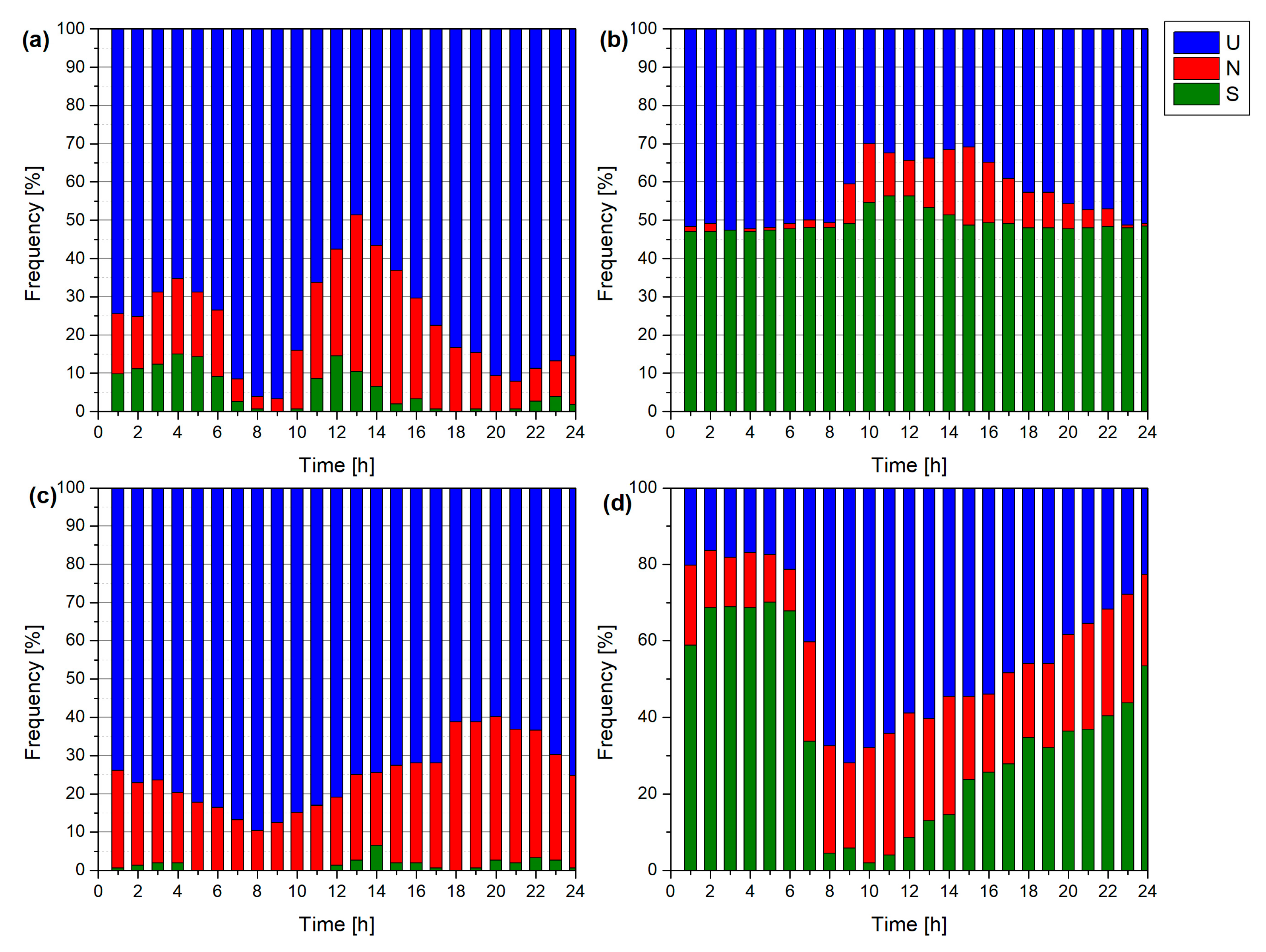
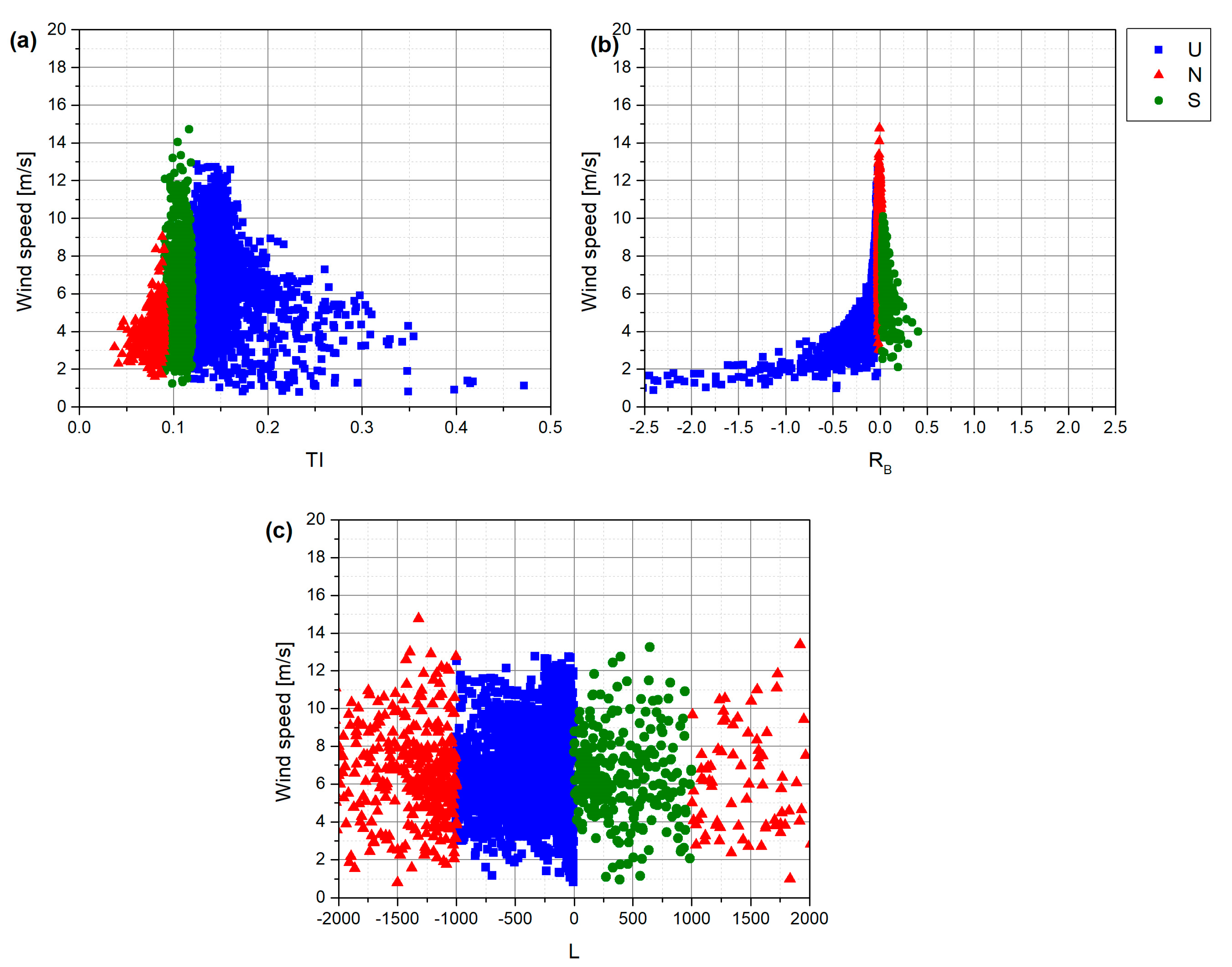
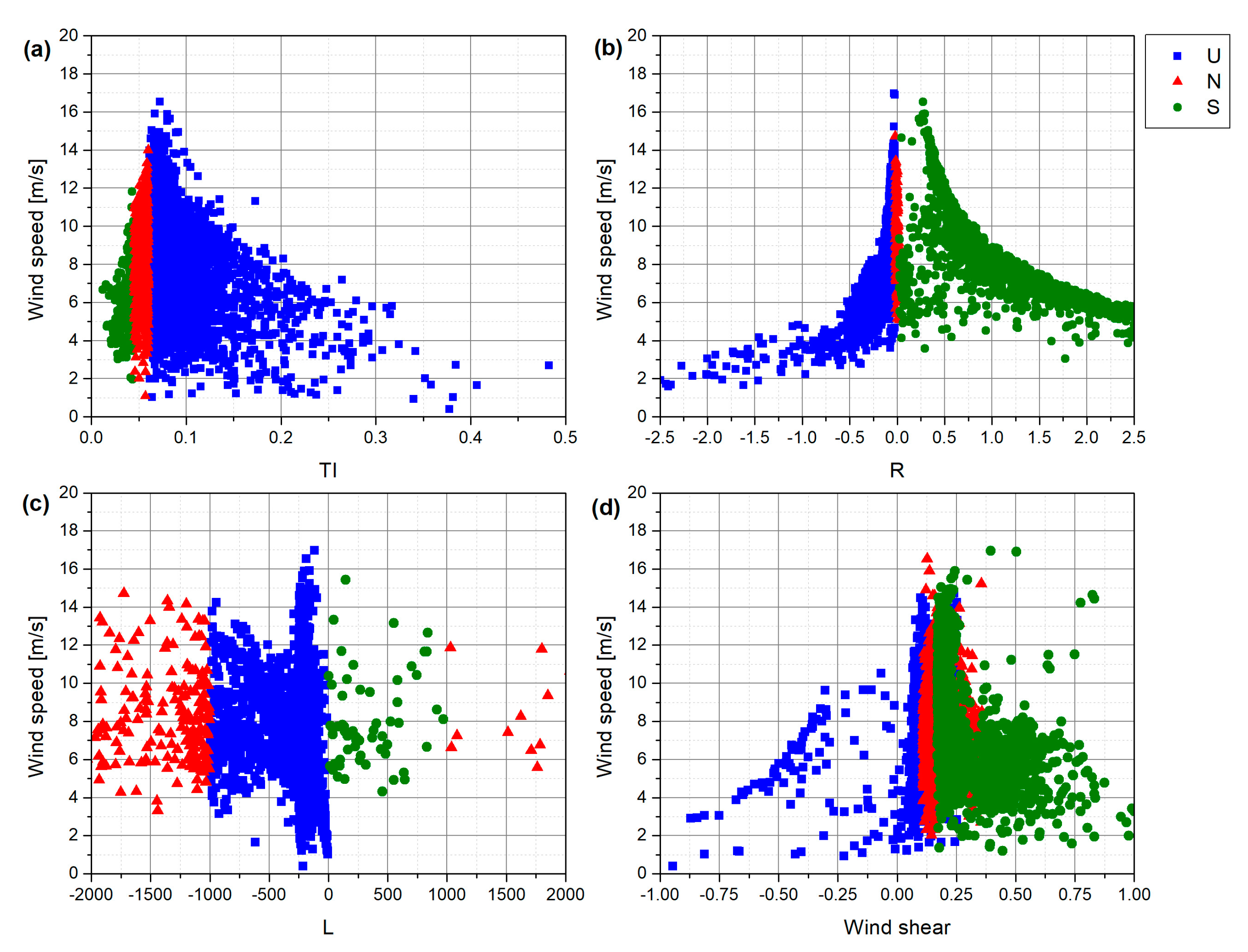
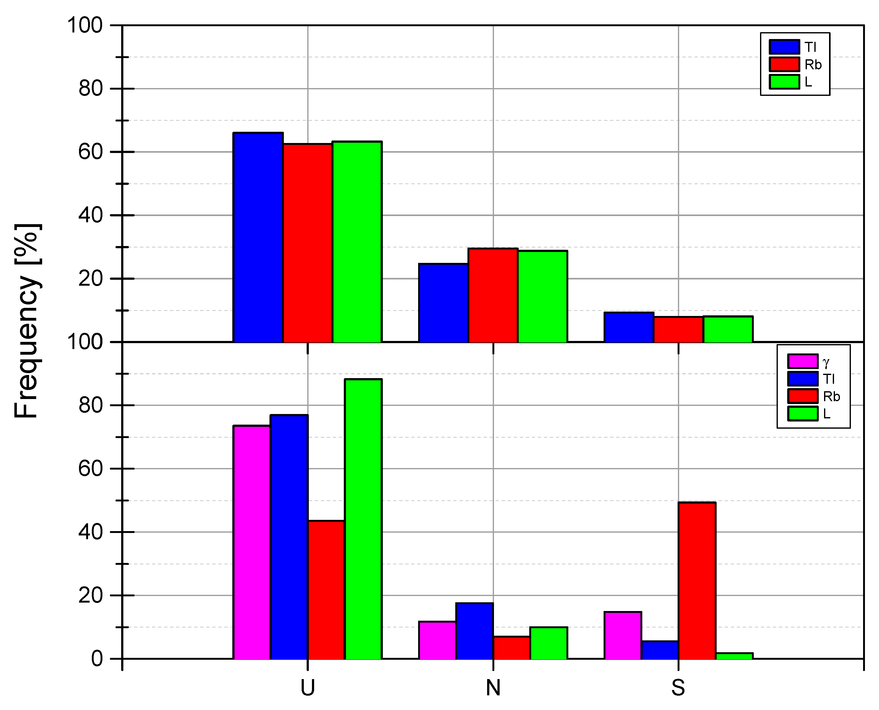
2.3. Atmospheric Stability Classification

Several direct parameters describe atmospheric stability, either from a qualitative or quantitative point of view. When the parameters estimate the atmospheric stability from the turbulence associated with the site, they are said to be indirect. On the other hand, they are direct when the atmospheric stability condition is determined directly from the corresponding parameter. Within the direct parameters are Monin–Obukhov length, Richardson number, Deacon number, and McVehil ratio. Within the indirect parameters are wind shear, turbulence intensity, and turbulent kinetic energy [14]. The choice of parameters depends on several factors, such as the specific problem to be solved, the available facilities and instruments, and the experimental limitations.

The four parameters used in the study will be detailed below.

2.3.1. Wind Shear

In the wind industry, indirect measurements are often used to describe atmospheric stability. One of them is the wind shear exponent $\left(\gamma \right),$ which indicates the existence or not of a stratified flow [39].

Wind speed measurements at two heights enable the calculation of this dimensionless exponent $\left(\gamma \right)$ from the power-law or Hellmann’s exponential profile [10,12,22,40,41,42,43], given by

$$\gamma =\frac{ln\left(U_2/U_1\right)}{ln\left(z_2/z_1\right)}.$$

(3)

Generally, for $\gamma$, a constant value of 0.143 is used for open terrain during the day and 0.5 during the night [43,44,45]. In this study, $z_2=50 \mathrm{m},z_1=20 \mathrm{m},$ and $U_{\left(z\right)}$ is the velocity at height $z$.

2.3.2. Turbulence Intensity

Another parameter used in wind projects is the turbulence intensity $\left(TI\right)$, since it quantifies variations in wind speed at short intervals [12,46]. This parameter describes in a general way the level of turbulence present in the average wind speed. $TI$ is given by the following equation [11,47]:

$$TI=\frac{\sigma }{\overline{U}}$$

(4)

where $\sigma$ is the standard deviation of the wind speed and $\overline{U}$ is the mean wind speed. This study found $TI$ at 20 m and 50 m.

2.3.3. Bulk Richardson Number

The “bulk Richardson number” $\left(R_B\right)$ is the simplest way to relate the vertical potential temperature difference within a height interval. $R_B$ relates the buoyancy energy to the kinetic energy of the wind shear through the following expression [48]:

$$R_B=\left(\frac{g}{{\theta }_{vs}}\right)\frac{{\theta }_v\left(z\right)-{\theta }_{vs}}{u{\left(z\right)}^2+v{\left(z\right)}^2}z,$$

(5)

where $z$ is the height above the ground, ${\theta }_{vs}$ is the virtual temperature near the surface, and $u\left(z\right),v\left(z\right)$ are the horizontal components of velocity measured at $z$.

For sea conditions, Equation (2) can be reduced if the virtual potential temperature is close to the air temperature and only the horizontal wind speed component exists $\left(u\right).$ Therefore, $R_B$ becomes

$$R_B=\frac{gz\left(T_a-T_s\right)}{\left(273.15+T_a\right)u^2}.$$

(6)

where $T_a$ is the air temperature and $T_s$ is the water temperature on the sea surface [26].

Since this study is carried out in a coastal area and the prevailing winds come from the ocean’s northwest and east, $R_B$ was calculated from Equation (6), using $T_a$ and $u$ data from TCP station and $T_s$ data from National Oceanic and Atmospheric Administration (NOAA) marine buoys [49]. The Yucatan Basin buoy is 222 km east-southeast (ESE) of Cozumel, Mexico, in the Caribbean Sea (Figure 2a). According to the statistical data of the buoy, the prevailing winds in the NOAA marine station Yucatan basin are from ENE to ESE, as illustrated in Figure 2b. The main characteristics of the buoy are presented in

Table 2. Characteristics of NOAA marine station used in this research.

	Yucatan Basin
Coordinates	19°49′12″ N 84°56′41″ W
Site elevation	Sea level
Averaging period	Hourly
Air temperature height	3.7 m above site elevation
Anemometer height	4.1 m above site elevation
Barometer elevation	2.7 m above mean sea level
Sea temperature–depth	1.5 m below the water line
Water depth	4554 m

.

2.3.4. Monin–Obukhov Length

The Monin–Obukhov length $\left(L\right)$ is the most commonly used aspect ratio to describe atmospheric stability. According to the Monin–Obukhov similarity theory $\left(MOST\right)$ [44], $L$ is also known as a scale parameter since it represents the relationship between mechanical and convective turbulence production. $L$ is obtained using:

$$L=-\frac{u_{*}^3{\theta }_v}{kg\left(\overline{{\omega }^{\prime }{\theta }^{\prime }}\right)}$$

(7)

where ${\theta }_v$ is the virtual potential temperature, $k$ is the Von Karman constant $\left(k\approx 0.4\right)$, $\overline{{\omega }^{\prime }{\theta }^{\prime }}$ is the kinematic sensible heat flux, and $u_{*}={\left({\overline{u^{\prime }{v}^{\prime }}}^2+{\overline{v^{\prime }{w}^{\prime }}}^2\right)}^{1/4}$ is the friction velocity or shearing stress [17,50,51].

$L$ is not widely used for wind energy assessment as it is only applied in short periods, and some required data are challenging to obtain.

With the value of $R_B$, it is possible to find $L$ through empirical expressions given by [27]:

$$\frac{z}{L}=\left\{\begin{array}{cc}{R}_B& R_B<0\\ \frac{R_B}{1-5R_B}& {0<R}_B<0.2\end{array}\right..$$

(8)

where $z$ is the measurement’s height. In this study, after finding $R_B$ as described in Section 2.3.3, Equation (8) is used to find $L$.

Table 3. Classification of atmospheric stability according to parameters used in this study.

Parameter	Equation	Atmospheric Conditions Range
$L$	$\mathrm{L}=-\frac{{\mathrm{u}}_{*}^3{\mathsf{\theta }}_{\mathrm{v}}}{\mathrm{k}\mathrm{g}\left(\overline{{\mathsf{\omega }}^{\prime }{\mathsf{\theta }}^{\prime }}\right)}$	U: $-L$ N: ∞ S: $+L$
$R_B$	${\mathrm{R}}_{\mathrm{B}}=\left(\frac{\mathrm{g}}{{\mathsf{\theta }}_{\mathrm{v}\mathrm{s}}}\right)\frac{{\mathsf{\theta }}_{\mathrm{v}}\left(\mathrm{z}\right)-{\mathsf{\theta }}_{\mathrm{v}\mathrm{s}}}{\mathrm{u}{\left(\mathrm{z}\right)}^2+\mathrm{v}{\left(\mathrm{z}\right)}^2}$ z	U: $R_B<-0.02$
		N: $-0.02\le R_B<0.02$ (quasineutral)
		S: $R_B>-0.02$
$\gamma$	$\frac{{\mathrm{u}}_2}{{\mathrm{u}}_1}={\left(\frac{{\mathrm{h}}_2}{{\mathrm{h}}_1}\right)}^{\mathsf{\gamma }}$	U: $\gamma <0.26$
		N: $0.26<\gamma <0.36$
		S: $\gamma \ge 0.36$
$TI$	$\mathrm{T}\mathrm{I}=\frac{\mathsf{\sigma }}{\overline{\mathrm{U}}}$	For 20 m: U: $TI>12\%$
		N: 9$\%<TI<12\%$
		S: $TI<9\%$
		For 50 m: U: $TI>6\%$
		N: $4.5\%<TI<6\%$
		S: $TI<4.5\%$

summarizes the parameters used in this study with their stability measurements and atmospheric conditions ranges. To define these ranges, previous studies were reviewed [22,24,26,52]. It is known that the same turbulence index derived from one height does not apply to a different height, and that differences of 20–30% have been reported in the literature [53,54,55]. For these heights (on average) in particular, and at the site of interest, the average was approximately 50%. This difference can be attributed to surface effects compared to other cases where the measurements are offshore (several kilometers from the shore). Therefore, an average value of 35–40% was used in this work to achieve convergence of the four parameters studied for each height.

2.4. Wind Energy Production

Annual energy production $\left(AEP\right)$ depends mainly on two factors: (i) the wind speed in the region and (ii) the power curve of the wind turbine, and can be expressed as

$$AEP=\sum _i{Pd\left(u\right)t}_i{P}_i$$

(9)

where $Pd\left(u\right)$ is the Weibull probability density function, $t_i$ is the time of occurrence of each interval of the wind speed, and $P_i$ is the value of the power obtained from the wind turbine power curve for each wind speed interval calculated with Equation (1).

When statistical distributions such as the Weibull probability density function are used, a condition of neutral stability is assumed to estimate the wind speed [11,46], leading to conservative estimates and, consequently, biased values of $AEP$ to those found experimentally. Therefore, according to the $MOST$ theory, it is possible to estimate wind speed, considering stability parameters to minimize errors in the calculation.

In the atmospheric boundary layer ($ABL$), the general expression to estimate the values of wind speed considering atmospheric stability is given by [28,56,57,58,59]

$$u_2=\frac{u_{*}}{k}\mathit{ln}\left(\frac{z}{z_0}\right)-\psi \left(\frac{z}{L}\right).$$

(10)

where $u_{*}$ is the friction velocity, the function $\psi \left(\frac{z}{L}\right)$ varies according to the atmospheric stability, and $z_0$ is the roughness length.

For a neutral atmosphere:

$$\psi \left(\frac{z}{L}\right)=0.$$

(11)

For unstable conditions, $z/L<0$, the Paulson’s equation is used [21,60]

$${\psi }_U\left(\frac{z}{L}\right)=-2\mathit{ln}\left(\frac{1+x}{2}\right)-\mathit{ln}\left(\frac{1+x^2}{2}\right)+2{\mathit{tan}}^{-1}\left(x\right)-\pi /2.$$

(12)

where

$$x={\left[1-\left(\frac{15z}{L}\right)\right]}^{1/4}.$$

(13)

For stable conditions $z/L>0$, the function $\psi \left(\frac{z}{L}\right)$ is represented by the Businger–Dyer equation [26,28]

$${\psi }_S\left(\frac{z}{L}\right)=\frac{4.7z}{L}.$$

(14)

where $z$ is the height and $L$ is the Monin–Obukhov length.

In this case, wind speed (Equation (10)) is found for each atmospheric stability condition according to Equations (11), (12) and (14), depending on whether the atmosphere is neutral, unstable, or stable, respectively. Subsequently, using the estimated wind speeds, $Pd\left(u\right)$ is found and, with Equation (9), the $AEP$ will be obtained for each of the proposed scenarios $(U,N,S)$.

The WES 30 wind turbine is used for modeling the $AEP$ at the site. The main characteristics of this wind turbine are presented in

Table 4. Datasheet of wind turbine WES 30.

System	Characteristic	Value
Power	Rated power	250 kW
	Cut-in wind speed	3 m/s
	Rated wind speed	13 m/s
	Cut-out wind speed	25 m/s
Rotor	Diameter	30 m
	Swept area	707 m2
	Number of blades	3
Generator	Voltage	400 V
	Grid frequency	50/60 Hz
Tower	Hub height	48 m

.

3. Results and Discussions

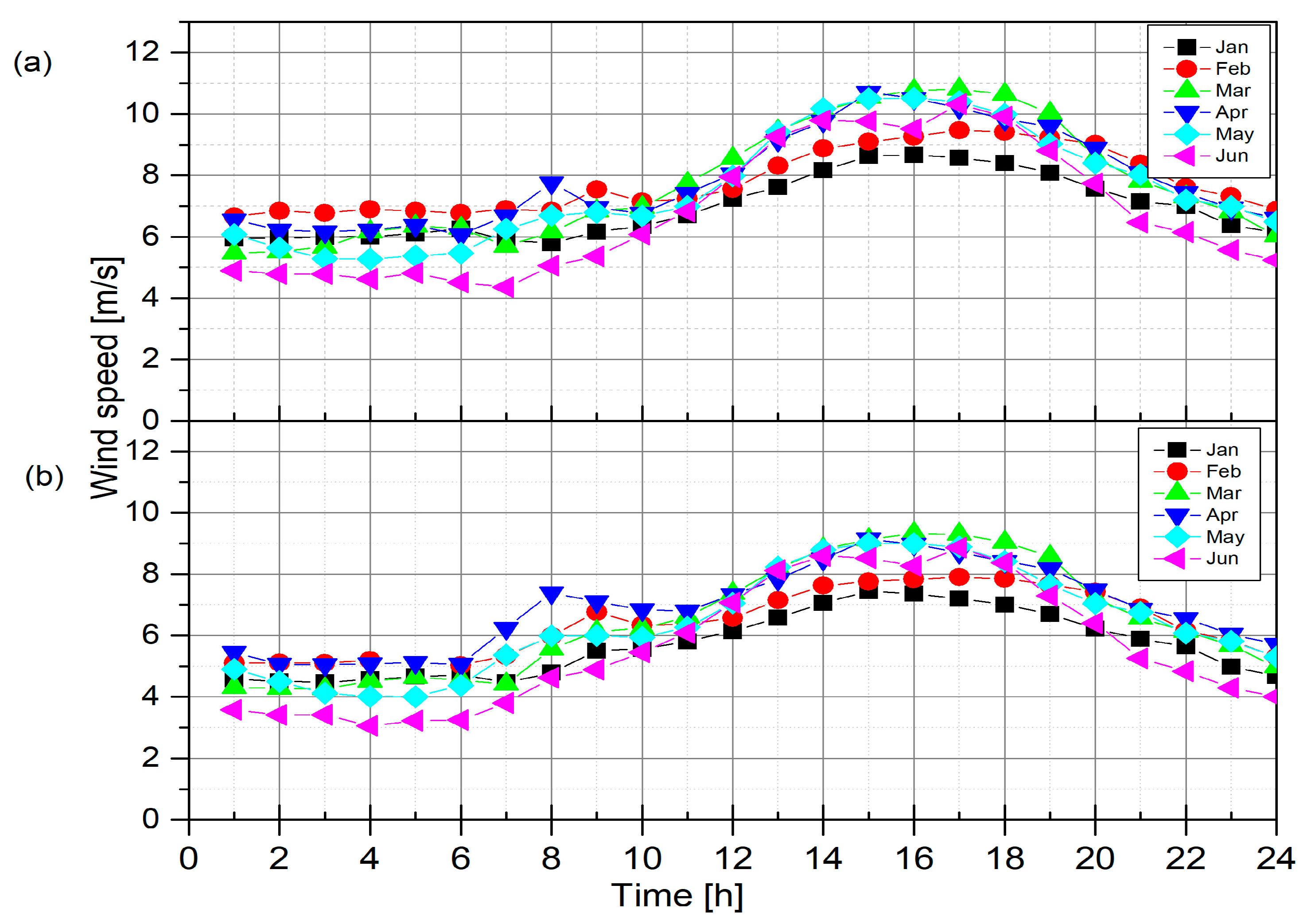
3.1. Wind Patterns

The wind speed diurnal pattern for the site at the two heights (50 m and 20 m) during the study months is presented in Figure 3. The highest wind speeds occur during the afternoon, between 14 h and 16 h. During this period, the thermal exchange between the land and sea air masses occurs, but it is also influenced by the local winds from the coastal zone.

The lowest wind speeds are generally obtained before sunrise, between 4 h and 7 h. Likewise, it is observed that this same diurnal behavior is independent of height since, although the mean wind speed is higher at 50 m than at 20 m, the same trend is observed.

Table 5. Wind speed and wind power density per month from the study site.

Month	20 m			50 m			WPD [W/m2]	Class
	Min [m/s]	Ave [m/s]	Max [m/s]	Min [m/s]	Ave [m/s]	Max [m/s]
January	0.15	5.69	14.07	0.23	6.95	29.67	205.52	2
February	0.98	6.39	12.37	0.83	7.78	13.68	289.09	2
March	0.42	6.49	13.18	0.57	7.76	28.53	286.23	2
April	0.53	6.87	15.87	0.21	7.87	29.42	298.46	2
May	0.40	6.40	13.34	0.28	7.57	26.65	265.58	2
June	0.15	5.61	12.55	0.54	6.77	14.51	190.23	1
Total period	0.44	6.24	13.56	0.44	7.45	23.74	255.85

summarizes the monthly average wind speeds for the entire monitoring period at the TCP station (January–June 2009). The difference between the monthly average speeds at 20 m and 50 m wind is about 1 m/s, and the difference between the maximum wind speeds is nearly 10 m/s in some months. The highest average wind speeds were measured in April, and the lowest wind speeds were measured in June for both heights. The highest average wind speeds occur between March and May on the Yucatan Peninsula. Therefore, the results are consistent with the expected values [61].

It was also possible to find, with measured data, the frequency distributions at the two heights, as illustrated in Figure 4. Figure 4 indicates lower wind speed values at 20 m, compared to those at 50 m, resulting from a positive shear. The wind speed modes are 5 m/s and 7 m/s for 20 m and 50 m, respectively. Both distributions span from 1 m/s to 16 m/s. As expected, when the measurement height increases, winds with higher speeds occur more frequently due to the absence of surrounding obstacles. Moreover, this behavior is typically observed in unstable conditions.

The wind is characterized by its speed and direction. Nevertheless, not all wind speeds produce energy. In general, for the blades of a wind turbine to rotate, moderate winds are needed, above 3 m/s and below 25 m/s. However, each machine is designed for a certain wind speed and turbulence intensity, from which the maximum corresponding power will be harvested. According to the wind power density calculated with Equation (2) in Table 5, there is a wind class 2 in the first five months and a wind class 1 in June. Therefore, the site is suitable for wind turbine deployment. However, the most significant uncertainty arises from the available wind energy estimation, which requires considering additional parameters. This will be addressed in the next section.

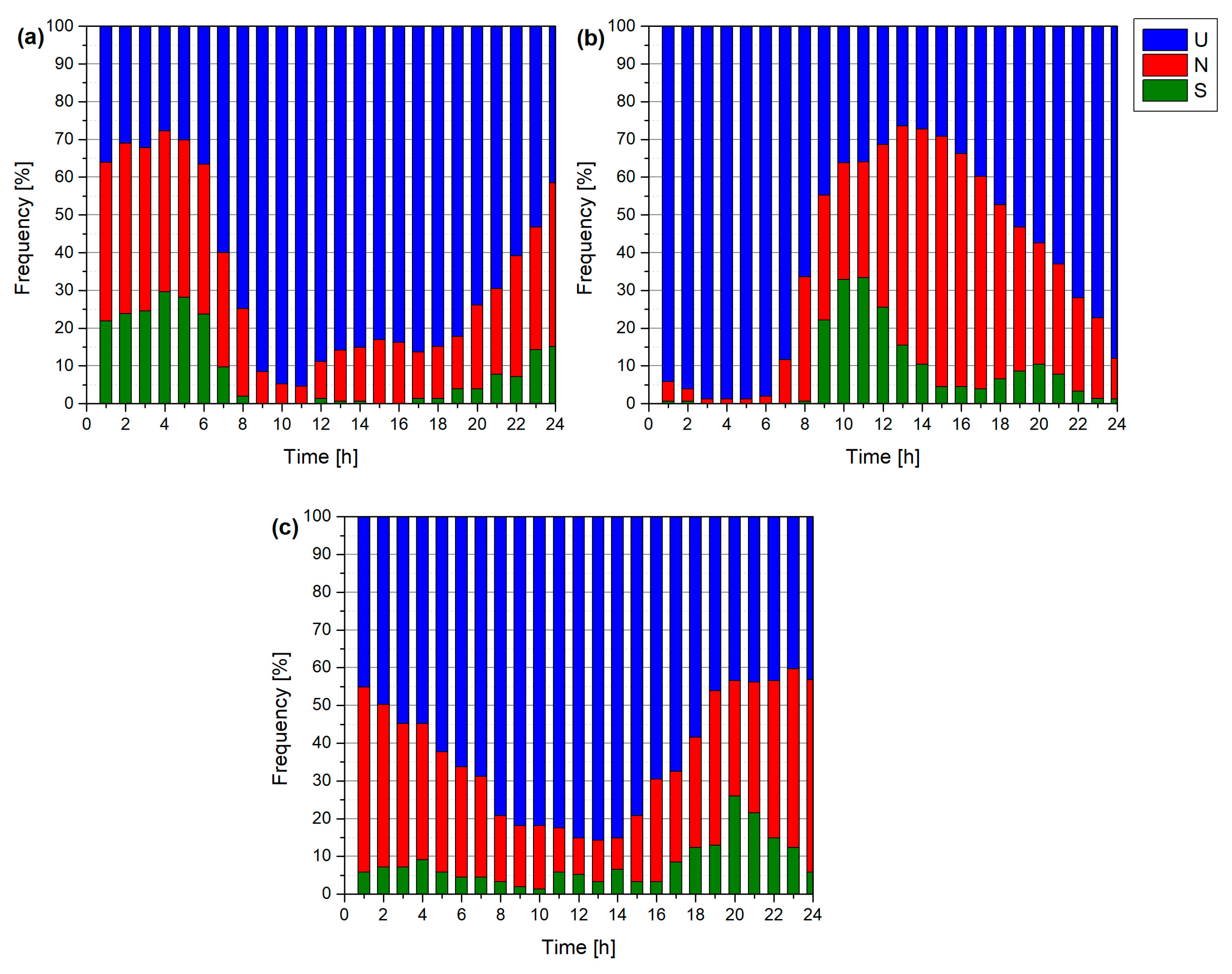
3.2. Atmospheric Stability

Atmospheric stability is one factor that determines the amount of energy available, for which some parameters are calculated. They indicate the atmospheric stability level at the site.

The frequency distribution of turbulence intensity at 20 m is presented in Figure 5a. Following the corresponding criteria established in Table 3 to define atmospheric stability in terms of $TI$, the periods in which the different atmospheric conditions were obtained in each hour are counted. Figure 5a presents a predominantly unstable atmosphere from 7 h to 23 h. At this height, neutral conditions represent about one-third of the nighttime hours. At dawn, neutral conditions prevail.

The transition between the thermal stability criteria during the day is gradual since there are no abrupt changes in the $TI$ values. Physically, the geographical conditions favor simultaneous thermal exchange between the vertical layers of the atmosphere and between the sea and the land.

The frequency distribution of $R_B$ over the day is also illustrated in Figure 5b for 20 m. Following the atmospheric stability criteria established in Table 3, it is observed that, at 20 m, there is a predominantly unstable atmosphere during low radiation conditions (early morning and night). At noon, there is an increasing presence of neutral atmospheric conditions and, as the sunset approaches, the atmosphere becomes more unstable.

Once the $R_B$ is obtained, $L$ can be found from Equation (8). The frequency distribution of $L$ over the day is illustrated in Figure 5c for 20 m. At this height, unstable atmospheric conditions predominate most of the day and, at midnight (between 23 h and 02 h), are neutral. Stable conditions at this height have a low occurrence.

The behavior observed at 50 m for $TI$ is presented in Figure 6a. In this case, an unstable atmosphere dominates all day since convective effects appear.

For $R_B$ at 50 m (Figure 6b), a stable atmosphere has the highest frequency only between 10 and 13 h. Therefore, there is not a predominant atmospheric condition.

For $L$ at 50 m, it is observed in Figure 6c that there is an unstable atmosphere most of the day and that a neutral atmosphere appears slightly until it reaches its maximum point between 18 and 20 h. Later, it returns to an unstable atmosphere.

For wind shear (Equation (3)), the diurnal pattern was obtained according to the average wind speed. Figure 6d illustrates the frequency distribution of wind shear. Following the criteria established in Table 3 to define atmospheric stability, there is a predominantly unstable atmosphere during the morning, until 7 a.m., and during the night, after 20 h. From 23 h to 6 h, a stable atmosphere prevails. Thus, an unstable atmosphere persists during the day at the study site. Lower values represent well-mixed atmospheric layers during mornings, coinciding with the moment when the average wind speed increases.

Figure 7a illustrates the dispersion of the $TI$ as a function of wind speed for 20 m. It is observed that there are lower $TI$ values at higher wind speeds. Therefore, the $TI$ is inversely proportional to the wind speed. Given that high turbulence values are related to power generation [12], this area is suitable for wind energy exploitation.

Moreover, it presents the data dispersion for the Richardson number (Figure 7b) corresponding to the wind speed at 20 m. According to Figure 8b, when speed exceeds 4 m/s, the $R_B$ values tend to be in the band of quasi-neutrality, while below this wind speed value, there are negative $R_B$ values that indicate an unstable atmosphere.

The data dispersion of Monin–Obukhov length (Figure 7c) at 20 m height wind speeds is presented. It is observed that a higher number of data points is found in the unstable atmosphere than in the stable atmosphere.

Figure 8a presents the $TI$ data dispersion at 50 m. It is observed that there are lower $TI$ values at higher wind speeds, and a higher number of data points are found in the unstable atmosphere.

Figure 8b reports that, below 6 m/s, the values of $R_B$ do not indicate a marked trend for any atmospheric condition. However, $R_B$ values tend to be quasi-neutral when wind speeds exceed 6 m/s. Figure 8c presents the data dispersion of the Monin–Obukhov length concerning the wind speed at 50 m. It is observed that a higher number of data points is found in the unstable atmosphere.

Figure 8d illustrates that lower wind shear values are less dispersed at higher wind speeds, while, at low speeds, high shear values are presented, and with a higher dispersion. A higher number of data points is found in the unstable atmosphere. Moreover, it is important to consider the close relationship between atmospheric turbulence and wind shear since low wind shear values lead to high turbulence values.

The classification of the atmosphere has been described separately for each parameter. Figure 9 illustrates the percentage of stable, unstable, and neutral periods at 20 m (top) and 50 m (bottom). For the height of 20 m, the three parameters ($TI,R_B,L$) have a predominantly unstable atmosphere (>50% of the total period), and similarly for 50 m, there is mostly (>50%) an unstable atmosphere with $\gamma$, $TI$ and $L$. For 50 m, $R_B$ described a stable atmosphere. However, the average occurrence percentage of each atmospheric stability condition for each height at the TCP station is higher in an unstable atmosphere.

Table 6. Average occurrence percentage of each atmospheric stability condition for each height at TCP station.

Atmospheric Condition	20 m [%]	50 m [%]
Unstable	67	64
Neutral	15	28
Stable	18	8

summarizes these observations.

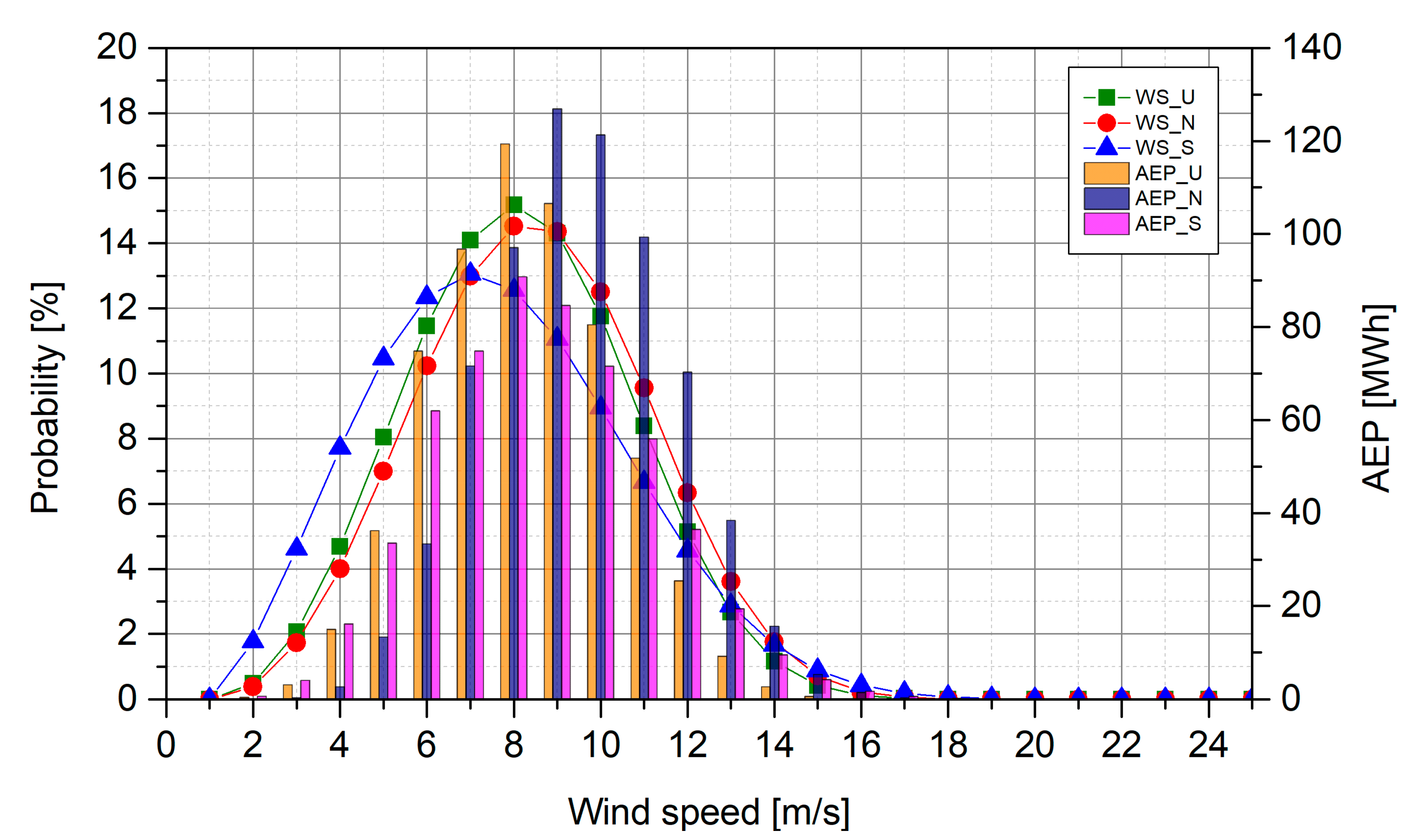
3.3. Energy Production

Once the atmospheric condition is defined, it is possible to determine the wind profile from Equation (10). The function $Pd\left(u\right)$ was calculated for the different wind profiles $\left(u_2\right)$ (Equation (10)) obtained at hub height according to $\psi \left(\frac{z}{L}\right)$, which represents the atmospheric stability condition that could be present on the site (Equations (11)–(13)). This is presented in Figure 10. This figure indicates that wind speeds between 6 m/s are more likely to occur under neutral and stable conditions. Under unstable and neutral conditions, the wind speed most often encountered is 7 m/s. It is also possible to find low-speed winds, but their probability percentage is less than 4%.

In addition, the same figure presents the estimated annual energy production $\left(AEP\right)$ using wind turbine WES 30 (see Table 4), corresponding to the three probability distributions for the different atmospheric conditions at the TCP station.

It is observed that, under unstable atmospheric conditions, there is a greater $AEP$, since it has a higher probability of occurrence at speeds greater than 7 m/s. Under a stable atmosphere, there is a lower estimate of the $AEP$, since the wind speeds that could occur according to $Pd\left(u\right)$ are lower. For stable atmospheric conditions, no significant difference is observed in contrast to the unstable atmosphere at wind speeds below 6 m/s. Although the wind turbine’s rated speed is not reached under any atmospheric condition, higher wind speeds can be found under neutral atmospheric conditions, which leads to greater energy production.

The capacity factor is the ratio between the energy produced by the turbine for one year and the estimated energy it would have if operated continuously at its nominal power.

Table 7. Operating parameters for wind turbine WES 30 on TCP station.

Condition Atmospheric	CF [%]	AEP [MWh]	% CF
Unstable	71	622.36	48
Neutral	79	697.41	12
Stable	63	566.20	11

reports in the first column the capacity factor $\left(CF\right)$ and in the second column the estimated annual energy production according to the correction realized to $u_2$ for each atmospheric condition that could be presented at the site. The third column of Table 7 shows the percentage that each $CF$ would have in the site according to the average occurrence of each atmospheric stability condition.

Although data is only available for six months, the estimate was made for one year of operation, considering that the wind probability distribution illustrated in Figure 4 is the same for one year. Since the wind resource assessment has already been extensively studied, it is known that a data series of at least one year is required. However, in this study, we do not focus on determining the wind resource present on the site but on analyzing the effects of atmospheric stability on energy production. Therefore, this analysis can be undertaken with the data available for 6 months.

Models in the wind industry generally use neutral stability to make the calculations of $AEP$ [22,23,24,25,26,27,28,29,30,31,32,33,34,35,36,37,38,39,40,41,42,43,44,45,46,47,48,49,50,51,52]. However, in this study, it was found that unstable conditions lead to a higher energy production than in stable conditions. In neutral conditions, the energy production was even higher than in unstable conditions. Under unstable conditions, the $AEP$ difference between unstable and neutral atmospheric considerations is around 8%. Moreover, the $AEP$ difference between stable and neutral atmospheric considerations is 16%, and between unstable and stable atmospheric considerations is around 8%. That is, considering a stable atmosphere instead of an unstable atmosphere, as occurred on the site, can lead to underestimations in the energy production, which leads to not being able to supply the energy production that the developers of the wind farms forecasted. However, if an utterly neutral atmosphere is assumed, overestimations can be obtained.

These results demonstrate the importance of considering atmospheric conditions for energy production. There are significant differences according to the atmospheric stability present at the site.

4. Conclusions

Changes in the wind industry have significantly involved aspects of other areas, such as meteorology, particularly atmospheric stability. Several methods to find the vertical profile need to consider this characteristic. Neglecting the atmospheric stability effect leads to misleading estimations of wind speeds at the site.

The present study used a remote station to measure wind speed at 20 and 50 m above sea level. Differences were found (≈1 m/s) between the mean average wind speeds obtained during the day and between the months of study for two heights. Additionally, differences of up to 10 m/s could be found among the maximum speeds in some months. Regarding the diurnal profile for both cases, the highest wind speeds were obtained in the afternoon (around 16 h).

Atmospheric stability was also analyzed for four atmospheric stability parameters: wind shear, $TI$, $R_B$ and $L$. The first two parameters are usually used in the wind industry, and the other two are in micrometeorology.

According to the $TI$ analysis, the site presents atmospheric instability at 20 m and 50 m. Wind shear was only calculated for 50 m and reported the site to have a predominantly unstable atmosphere.

Additionally, using data from marine buoys and masts, the other two stability parameters were calculated, $R_B$ and $L$. These two parameters at both heights corroborated and cross-validated the prevailing condition on the interest site (mostly unstable). The results indicated that the assumptions considered for this site are valid.

With the data obtained, it was possible to estimate wind speeds considering the three atmospheric conditions to ultimately calculate the $AEP$ that could be obtained from one wind turbine model. Differences of 16% were found between the $AEP$ produced under a stable and unstable atmosphere, and differences of 8% between the $AEP$ produced under a neutral and unstable atmosphere. That is, if a stable atmosphere is considered, there would be an underestimation of $AEP$ and an overestimation if the site is deemed to have a neutral atmosphere.

Therefore, the importance of considering the conditions of atmospheric stability in wind power estimation modeling in any site study can be reaffirmed to avoid biases in energy production estimates. By considering these atmospheric conditions, power producers will be able to count on more precise tools to forecast the wind potential, which, as observed in this study, affects the estimation of energy that can be produced. Manufacturers can also benefit from this analysis since atmospheric stability affects the mechanical loads on wind turbines or the risk of failure due to fatigue and incorporate control systems that can improve the performance of wind turbines.

In the future, the risks of not having precise estimation methods that incorporate atmospheric stability parameters in energy production will be quantified economically. In addition, the periods of higher energy production will be related to the corresponding periods of stability. This work can be used as a reference for incorporating these stability parameters into energy production models using novel estimation techniques such as neural networks and machine learning, among others.

References

1. BP. Statistical Review of World Energy 2021; BP: London, UK, 2021. [Google Scholar]
2. IRENA. Renewable Power Generation Costs in 2020; Abu Dabhi, International Renewable Energy Agency: Abu Dabhi, United Arab Emirates, 2020. [Google Scholar]
3. REN 21. Renewables 2021. Global Status Report; REN21 Secretariat: Paris, France, 2021. [Google Scholar]
4. GWEC. Global Wind Report 2021; Lobal Wind Energy Council: Brussels, Belgium, 2021. [Google Scholar]
5. SENER. Prospectiva del Sector Eléctrico 2018–2032; Secretaría de Energía: Mexico city, Mexico, 2018. [Google Scholar]
6. Bracho, R.; Flores-Espino, F.; Morgenstein, J.; Aznar, A.; Castillo, R.; Settle, E. The Yucatan Peninsula Energy Assessment: Pathways for a Clean and Sustainable Power System; National Renewable Energy Laboratory: Golden, CO, USA, 2021. [Google Scholar]
7. REVE Wind Energy in Yucatan, Vive Energía Inaugurates the Peninsula Wind Farm. Available online: https://www.evwind.es/2020/08/04/wind-energy-in-yucatan-vive-energia-inaugurates-the-peninsula-wind-farm/76230 (accessed on 6 March 2023).
8. REVE Wind Energy in Yucatan: Inaugurate Dzilam Bravo Wind Farm with 66 Wind Turbines. Available online: https://www.evwind.es/2019/05/04/wind-energy-in-yucatan-inaugurate-dzilam-bravo-wind-farm-with-66-wind-turbines/67037 (accessed on 1 March 2023).
9. Yucatan Magazine New Wind Farm Is Yucatan’s 5th Clean-Energy Site. Available online: https://yucatanmagazine.com/new-wind-farm-is-yucatans-5th-clean-energy-site/ (accessed on 1 March 2023).
10. Hulio, Z.H.; Jiang, W.; Rehman, S. Techno—Economic Assessment of Wind Power Potential of Hawke’s Bay Using Weibull Parameter: A Review. Energy Strategy Rev. 2019, 26, 100375. [Google Scholar] [CrossRef]
11. Pramod, J. Wind Energy Engineering, 2nd ed.; McGraw Hill: New York, NY, USA, 2016; ISBN 9780071714785. [Google Scholar]
12. Murthy, K.S.R.; Rahi, O.P. A Comprehensive Review of Wind Resource Assessment. Renew. Sustain. Energy Rev. 2017, 72, 1320–1342. [Google Scholar] [CrossRef]
13. Stull, R.B. An Introduction to Boundary Layer Meteorology; Stull, R.B., Ed.; Springer: Dordrecht, The Netherlands, 1988; ISBN 978-90-277-2769-5. [Google Scholar]
14. Pérez Albornoz, C.; Escalante Soberanis, M.A.; Ramírez Rivera, V.; Rivero, M. Review of Atmospheric Stability Estimations for Wind Power Applications. Renew. Sustain. Energy Rev. 2022, 163, 112505. [Google Scholar] [CrossRef]
15. IEC. Wind Energy Generation Systems—Part 12-1: Power Performance Measurements of Electricity Producing Wind Turbines; International Electrotechnical Comission: Geneva, Switzerland, 2017. [Google Scholar]
16. Gualtieri, G. A Comprehensive Review on Wind Resource Extrapolation Models Applied in Wind Energy. Renew. Sustain. Energy Rev. 2019, 102, 215–233. [Google Scholar] [CrossRef]
17. Holtslag, M.C.; Bierbooms, W.A.A.M.; Bussel, G.J.W. van Estimating Atmospheric Stability from Observations and Correcting Wind Shear Models Accordingly. J. Phys. Conf. Ser. 2014, 555, 012052. [Google Scholar] [CrossRef]
18. Ren, G.; Liu, J.; Wan, J.; Li, F.; Guo, Y.; Yu, D. The Analysis of Turbulence Intensity Based on Wind Speed Data in Onshore Wind Farms. Renew. Energy 2018, 123, 756–766. [Google Scholar] [CrossRef]
19. Roy, S.B.; Sharp, J. Why Atmospheric Stability Matters in Wind Assessment. Available online: https://nawindpower.com/online/issues/NAW1301/FEAT_06_Why_Atmospheric.html (accessed on 19 December 2019).
20. Sumner, J.; Masson, C. Influence of Atmospheric Stability on Wind Turbine Power Performance Curves. J. Sol. Energy Eng. 2006, 128, 531–538. [Google Scholar] [CrossRef]
21. Han, X.; Liu, D.; Xu, C.; Shen, W.Z. Atmospheric Stability and Topography Effects on Wind Turbine Performance and Wake Properties in Complex Terrain. Renew. Energy 2018, 126, 640–651. [Google Scholar] [CrossRef]
22. St. Martin, C.M.; Lundquist, J.K.; Clifton, A.; Poulos, G.S.; Schreck, S.J. Wind Turbine Power Production and Annual Energy Production Depend on Atmospheric Stability and Turbulence. Wind Energy Sci. 2016, 1, 221–236. [Google Scholar] [CrossRef]
23. Bardal, L.M.; Sætran, L.R.; Wangsness, E. Performance Test of a 3MW Wind Turbine—Effects of Shear and Turbulence. Energy Procedia 2015, 80, 83–91. [Google Scholar] [CrossRef]
24. Kim, D.-Y.; Kim, Y.-H.; Kim, B.-S. Changes in Wind Turbine Power Characteristics and Annual Energy Production Due to Atmospheric Stability, Turbulence Intensity, and Wind Shear. Energy 2021, 214, 119051. [Google Scholar] [CrossRef]
25. Peña, A.; Hahmann, A.N. Atmospheric Stability and Turbulence Fluxes at Horns Rev-an Intercomparison of Sonic, Bulk and WRF Model Data. Wind Energy 2012, 15, 717–731. [Google Scholar] [CrossRef]
26. Bahamonde, M.I.; Litrán, S.P. Study of the Energy Production of a Wind Turbine in the Open Sea Considering the Continuous Variations of the Atmospheric Stability and the Sea Surface Roughness. Renew. Energy 2019, 135, 163–175. [Google Scholar] [CrossRef]
27. Bardal, L.M.; Onstad, A.E.; Sætran, L.R.; Lund, J.A. Evaluation of Methods for Estimating Atmospheric Stability at Two Coastal Sites. Wind Eng. 2018, 42, 561–575. [Google Scholar] [CrossRef]
28. Gualtieri, G.; Secci, S. Comparing Methods to Calculate Atmospheric Stability-Dependent Wind Speed Profiles: A Case Study on Coastal Location. Renew. Energy 2011, 36, 2189–2204. [Google Scholar] [CrossRef]
29. Kim, D.-Y.; Kim, B.-S. Differences in Wind Farm Energy Production Based on the Atmospheric Stability Dissipation Rate: Case Study of a 30 MW Onshore Wind Farm. Energy 2022, 239, 122–380. [Google Scholar] [CrossRef]
30. Lim, H.-C. Atmospheric Stability of Surface Boundary Layer in Coastal Region of the Wol–Ryong Site. Phys. A Stat. Mech. Its Appl. 2012, 391, 3875–3884. [Google Scholar] [CrossRef]
31. Radünz, W.C.; Sakagami, Y.; Haas, R.; Petry, A.P.; Passos, J.C.; Miqueletti, M.; Dias, E. Influence of Atmospheric Stability on Wind Farm Performance in Complex Terrain. Appl. Energy 2021, 282, 116–149. [Google Scholar] [CrossRef]
32. Soler-Bientz, R.; Watson, S.; Infield, D. Preliminary Study of Long-Term Wind Characteristics of the Mexican Yucatán Peninsula. Energy Convers. Manag. 2009, 50, 1773–1780. [Google Scholar] [CrossRef]
33. Soler-Bientz, R.; Watson, S.; Infield, D. Wind Characteristics on the Yucatán Peninsula Based on Short Term Data from Meteorological Stations. Energy Convers. Manag. 2010, 51, 754–764. [Google Scholar] [CrossRef]
34. Soler-Bientz, R. Preliminary Results from a Network of Stations for Wind Resource Assessment at North of Yucatan Peninsula. Energy 2011, 36, 538–548. [Google Scholar] [CrossRef]
35. Cedar Lake Ventures Climate and Average Weather Year Round in Telchac Puerto. Available online: https://weatherspark.com/y/12404/Average-Weather-in-Telchac-Puerto-Mexico-Year-Round (accessed on 3 March 2023).
36. Google Maps Localization of Measurement Station Telchac Puerto. Available online: https://google-earth.gosur.com (accessed on 25 April 2022).
37. AWS Scientific. Wind Resource Assessment Handbook; AWS Scientific: Golden, CO, USA, 1997. [Google Scholar]
38. Ibrahim, M.Z.; Yong, K.H.; Ismail, M.; Albani, A. Spatial Analysis of Wind Potential for Malaysia. Int. J. Renew. Energy Res. 2015, 5, 201–209. [Google Scholar] [CrossRef]
39. Wharton, S.; Lundquist, J.K. Assessing Atmospheric Stability and Its Impacts on Rotor-Disk Wind Characteristics at an Onshore Wind Farm. Wind Energy 2012, 15, 525–546. [Google Scholar] [CrossRef]
40. Bañuelos Ruedas, F.; Angeles Camacho, C.; Serrano García, J.A.; Muciño Morales, D.E. Análisis y Validación de Metodología Usada Para La Obtención de Perfiles de Velocidad de Viento. In Proceedings of the REUNIÓN DE VERANO, RVP-AI’2008, Acapulco, Guerrero, Mexico, 6–12 July 2008; IEEE Sección México: Acapulco, Guerrero, Mexico, 2008; pp. 1–8. [Google Scholar]
41. Chaurasiya, P.K.; Ahmed, S.; Warudkar, V. Wind Characteristics Observation Using Doppler-SODAR for Wind Energy Applications. Resour. -Effic. Technol. 2017, 3, 495–505. [Google Scholar] [CrossRef]
42. Gualtieri, G. Atmospheric Stability Varying Wind Shear Coefficients to Improve Wind Resource Extrapolation: A Temporal Analysis. Renew. Energy 2016, 87, 376–390. [Google Scholar] [CrossRef]
43. Kubik, M.L.; Coker, P.J.; Barlow, J.F.; Hunt, C. A Study into the Accuracy of Using Meteorological Wind Data to Estimate Turbine Generation Output. Renew. Energy 2013, 51, 153–158. [Google Scholar] [CrossRef]
44. Göçmen, T.; Van Der Laan, P.; Réthoré, P.-E.; Diaz, A.P.; Larsen, G.C.; Ott, S. Wind Turbine Wake Models Developed at the Technical University of Denmark: A Review. Renew. Sustain. Energy Rev. 2016, 60, 752–769. [Google Scholar] [CrossRef]
45. Newman, J.; Klein, P. The Impacts of Atmospheric Stability on the Accuracy of Wind Speed Extrapolation Methods. Resources 2014, 3, 81–105. [Google Scholar] [CrossRef]
46. Manwell, J.F.; McGowan, J.G.; Rogers, A.L. Wind Energy Explained, 2nd ed.; Wiley: Chichester, UK, 2009; ISBN 9780470015001. [Google Scholar]
47. Kumer, V.-M.; Reuder, J.; Dorninger, M.; Zauner, R.; Grubišić, V. Turbulent Kinetic Energy Estimates from Profiling Wind LiDAR Measurements and Their Potential for Wind Energy Applications. Renew. Energy 2016, 99, 898–910. [Google Scholar] [CrossRef]
48. Stull, R. Practical Meteorology: An Algebra-Based Survey of Atmospheric Science; 1.02b; Roland Stull: Vancouver, BC, Canada, 2017; ISBN 9780888652836. [Google Scholar]
49. NOAA Historical Data. Available online: https://www.ndbc.noaa.gov/ (accessed on 30 September 2022).
50. Barthelmie, R.J.; Churchfield, M.J.; Moriarty, P.J.; Lundquist, J.K.; Oxley, G.S.; Hahn, S.; Pryor, S.C. The Role of Atmospheric Stability/Turbulence on Wakes at the Egmond Aan Zee Offshore Wind Farm. J. Phys. Conf. Ser. 2015, 625, 012002. [Google Scholar] [CrossRef]
51. Monin, A.S.; Obukhov, A.M. Basic Laws of Turbulent Mixing in the Surface Layer of the Atmosphere. Tr. Akad. Nauk. SSSR Geophiz. Inst. 1959, 24, 163–187. [Google Scholar]
52. Wharton, S.; Lundquist, J.K. Atmospheric Stability Affects Wind Turbine Power Collection. Environ. Res. Lett. 2012, 7, 014005.31. [Google Scholar] [CrossRef]
53. Cheung, L.C.; Premasuthan, S.; Davoust, S.; von Terzi, D. A Simple Model for the Turbulence Intensity Distribution in Atmospheric Boundary Layers. J. Phys. Conf. Ser. 2016, 753, 032008. [Google Scholar] [CrossRef]
54. Marek, P.; Grey, T.; Hay, A. A Study of the Variation in Offshore Turbulence Intensity around the British Isles. In Proceedings of the Wind Europe Summit 2016, Hamburg, Germany, 27–29 September 2016. [Google Scholar]
55. Sletvold Øistad, I. Analysis of the Turbulence Intensity at Skipheia Measurement Station; Norwegian University of Science and Technology: Trondheim, Norway, 2015. [Google Scholar]
56. Guevara Díaz, J.M. Cuantificación del Perfil del Viento Hasta 100 m de Altura Desde la Superficie y Su Incidencia en la Climatología Eólica. Terra Nueva Etapa 2013, XXIX, 81–101. [Google Scholar]
57. Motta, M.; Barthelmie, R.J.; Vølund, P. The Influence of Non-Logarithmic Wind Speed Profiles on Potential Power Output at Danish Offshore Sites. Wind Energy 2005, 8, 219–236. [Google Scholar] [CrossRef]
58. Sathe, A.; Gryning, S.-E.; Peña, A. Comparison of the Atmospheric Stability and Wind Profiles at Two Wind Farm Sites over a Long Marine Fetch in the North Sea. Wind Energy 2011, 14, 767–780. [Google Scholar] [CrossRef]
59. Stevens, R.J.A.M.; Meneveau, C. Flow Structure and Turbulence in Wind Farms. Annu. Rev. Fluid Mech. 2017, 49, 311–339. [Google Scholar] [CrossRef]
60. Paulson, C.A. The Mathematical Representation of Wind Speed and Temperature Profiles in the Unstable Atmospheric Surface Layer. J. Appl. Meteorol. 1970, 9, 857–861. [Google Scholar] [CrossRef]
61. Soler-Bientz, R.; Watson, S.; Infield, D. Evaluation of the Wind Shear at a Site in the North-West of the Yucatan Peninsula, Mexico. Wind Eng. 2009, 33, 93–107. [Google Scholar] [CrossRef]
Figure 1. Measurement mast at the Telchac Puerto location. (a) Satellite view and (b) local area [36].
Energies 16 04134 g001
Figure 2. (a) Location of NOAA marine station Yucatan basin used in this research and (b) wind roses for NOAA marine station Yucatan basin.
Energies 16 04134 g002
Figure 3. Diurnal wind speed patterns for each month of the study at (a) 50 m and (b) 20 m.
Energies 16 04134 g003
Figure 4. Wind speed frequency distribution at 20 m and 50 m at TCP station.
Energies 16 04134 g004
Figure 5. Frequency distribution of (a) turbulence intensity, (b) Richardson bulk number, and (c) Monin–Obukhov length for a typical day at 20 m at TCP station.
Energies 16 04134 g005
Figure 6. Frequency distribution of (a) turbulence intensity, (b) Richardson bulk number, (c) Monin–Obukhov length, and (d) wind shear for a typical day at 50 m at TCP station.
Energies 16 04134 g006
Figure 7. Scatter plot of (a) turbulence intensity, (b) Richardson bulk number, and (c) Monin-Obukhov length for a typical day at 20 m at TCP station.
Energies 16 04134 g007
Figure 8. Scatter plot of (a) turbulence intensity, (b) Richardson bulk number, (c) Monin-Obukhov length, and (d) wind shear for a typical day at 50 m at TCP station.
Energies 16 04134 g008
Figure 9. Percentage of periods classified as unstable (U), neutral (N), and stable (S) according to instability parameters for 20 m (top) and 50 m (bottom).
Energies 16 04134 g009
Figure 10. Estimated annual energy production versus different wind speeds according to atmospheric stability.
Energies 16 04134 g010