Application of Particle Image Velocimetry and Computational Fluid Dynamics Methods for Analysis of Natural Convection over a Horizontal Heating Source

Abstract

The objective of this article is to address the challenges associated with visualizing air flow over a heating source in an open laboratory environment. The study uses a combination of experimental visualization and numerical simulation techniques to generate a 3D model of the air flow and heat transfer between the heating source and the environment via natural convection. The Particle Image Velocimetry method is used to experimentally visualize the air flow, which is known for its benefits of high speed and accuracy, and for its ability to avoid disturbing the flow of the fluid being investigated. The data obtained from this experimental method are used as input for numerical simulations using the Ansys Fluent program. The numerical simulations identify air vortices and other elements that disrupt the airflow in the laboratory environment. The resulting 3D model accurately represents the actual situation in the laboratory and could be further optimized by adjusting parameters such as the output of the heater and the heating source temperature. These parameters play a crucial role in ensuring thermal comfort in the laboratory environment, which is of utmost importance for user comfort. In conclusion, the study provides valuable insights into the visualization of air flow over a heating source and demonstrates the effectiveness of combining experimental and numerical simulation techniques to generate accurate 3D models of air flow and heat transfer.

1. Introduction

The quality of the environment has become a significant concern in recent times due to its impact on human health. The air flow within interiors, where people spend a large portion of their day, is influenced by various sources, such as heating, air conditioning, and ventilation [1]. The airflow affects thermal comfort and the concentration of pollutants in the air [2].

Optical methods, which has seen an unprecedented increase in computational and acquisition technologies in recent years, such as Particle Image Velocimetry (PIV), can be used to analyse the air flow within interiors. PIV is a non-contact method that captures the instantaneous velocity and properties of fluid flow by recording the time position of trace particles in the air flow.

This article focuses on visualizing the airflow over the surface of a heating source that uses natural convection to transfer heat to the laboratory environment. The heat from the heating foil affects the thermal comfort in the laboratory. The aim of the study is to measure the air speed above the surface of the heating foil experimentally at its maximum performance using PIV optical method and to create a numerical simulation based on these experimental data. The simulation is then used to optimize the air parameters to ensure user thermal comfort within the laboratory.

Natural convective flow occurs in fluids due to density gradients that are in turn developed due to temperature differences in the fluid. Accordingly, free or natural convection has been studied using similarity theory [3], integral theory [4], and by using experiments [5].

The analysis of natural convection from oriented heat exchange walls is the basis of heat transfer books and forms the starting point for research in this field [6,7,8]. The way of solution of natural convection occurs over a horizontal plate is different from how it occurs around a vertical plate. The mechanism for this is known as indirect natural convection [9], which is explained in detail for example in the work of Guha and Pradhan [10].

Thermal and velocity boundary layers are typical for convective flow. The presence of boundary layers in this type of flow was confirmed by Stewartson [11]. Researchers, such as Chen et al. [12] and Ghiaasiaan [6], have studied the dependencies of the Nusselt number as a function of Prandtl and Grashof numbers. They found that the velocity boundary layer is thicker than the thermal boundary layer only when the Prandtl number is large (Pr > 1). If the Prandtl number is close to 1 (Pr < 1, Pr = 1)), the boundary layers are of comparable thickness.

Numerous papers on computational fluid dynamics (CFD), which uses basic transport, state equations of fluid mechanics and criterion equations [13], have focused on natural convection [14] over a heated horizontal plate. These papers delve into the fundamental physical and thermodynamic understanding of natural convection. Guha and Sengupta [15] used post-processing of the CFD simulations to show the quantitative details of the 3D velocity and temperature fields, depending on the model geometry. In the work of Guha, Jain, and Pradhan [16], a CFD study of natural convection around heated inclined plates was conducted. The study provided an understanding of the contours of velocity, temperature, and pressure as a function of inclination angle over the entire range from vertical to horizontal and the calculation of the Nusselt number.

In addition, natural convection is a crucial phenomenon that appears in many technological devices, particularly in heat sources and climatization. Research in these areas needs to continue to ensure user comfort and improve the quality of the environment.

Natural Convection and Its Boundary Layers

Convective heat transfer is the transfer of heat through a fluid in motion, also called convection. The process of convective heat transfer involves the transfer of both enthalpy and kinetic energy resulting from the large-scale movement of the fluid- macroscopic movement [17].

Typically, convective heat transfer happens in the presence of a solid surface and a moving fluid, wherein a layer of fluid near the surface experiences a temperature change either by heating or cooling owing to the difference in temperature between it and the surrounding fluid. The disparity in density produced due to the temperature change creates a buoyancy force, which propels the movement of fluid flow close to the surface. This process is called free or natural convection, where the fluid behind the heated or cooled layer remains stationary (zero velocity) with a constant temperature [8,18].

When studying natural convection, the boundary layer theory is utilized, which employs comparable physical laws and techniques as those used in forced convection analysis. However, it is essential to factor in buoyancy forces while creating the momentum equation, and the boundary conditions are distinct [19,20]. During natural convection, the solid surface and the boundary layer’s edge remain motionless, while the bulk fluid remains at rest [8].

The nature of the flow in natural convection is determined based on the Grashof number, which is a dimensionless quantity. This number, represented by Gr, is calculated by comparing the buoyancy force to the viscous force in a fluid and is given by the following equation:

$$\mathrm{Gr}=\frac{L^{3}g\beta \Delta T}{{\nu }^2}$$

(1)

The Grashof number is used to predict the onset of natural convection in a fluid. When the Grashof number is less than a critical value, the flow in the fluid is dominated by the viscosity of the fluid, and conduction is the primary mode of heat transfer. When the Grashof number is greater than the critical value, buoyancy forces become significant, and natural convection occurs.

The Grashof number is an important parameter in many engineering applications, including heat exchangers, cooling systems, and geothermal energy.

The velocity field of the fluid in natural convection is reliant on the temperature, which necessitates iterative computations for analysis [21].

Four different categories of natural convection can transpire around a horizontal plate, and the classification of each group depends on the relative temperature of the plate’s surface with respect to the flowing fluid around it. It is essential to adapt the relations of natural convection for each type, as well as determining the direction of fluid flow towards the surface [22].

Figure 1 illustrates the four types of natural convection around a horizontal plate. In cases where the surface is hot and isolated from the upper side, the fluid tends to rise, but the plate’s presence hinders the upward flow, forcing the fluid to move around the plate before flowing freely around the edges (Figure 1a). Similarly, in Figure 1b, the temperature of the plate is cooler than the surrounding fluid, causing the flow to be directed downwards. Conversely, in Figure 1c,d, the plate’s temperature is warmer than the fluid, causing the fluid to move upwards and downwards, respectively.

The focus of this work is on a specific situation where a heating foil is situated on a desk, and the air flows over this heating source. It is crucial to determine the type of natural convection occurring in this scenario to optimize the heating efficiency and ensure proper ventilation. By analysing the temperature of the heating source relative to the surrounding fluid and the direction of fluid flow towards the surface, one can determine the appropriate relations for natural convection and make informed decisions regarding heating optimization.

2. Visualization Methods

The text elucidates two approaches to observe the airflow above a heating plate: experimental method called Particle Image Velocimetry (PIV) and a computational method involving numerical simulation using Ansys Fluent. The objective was to collect information on the velocity vectors of air present above the heating foil.

2.1. Measuring Airflow through Particle Image Velocimetry

The non-contact optical technique, PIV, is utilized to compute fluid velocity. This method necessitates injecting minute tracer particles into the fluid stream and then exposing the fluid to intense illumination.

The tracer particles move along with the fluid and reflect light, which is captured by imaging devices. The PIV method determines the rate of motion of the tracer particles instead of the fluid stream, as the tracer particles function as data carriers. The accuracy of the PIV technique depends on the selection and incorporation of the tracer particles into the fluid, as the particles are recorded in images and their local velocities are analysed using computer software [23,24].

The size of the tracer particles is critical to the accuracy of the PIV method, as they must be large enough to monitor the fluid flow and to reliably capture the small turbulences of the current structure. However, the particles must not be too small, as their scattered light may not be captured by the scanning technique. To sum up, the PIV technique includes the introduction of tracer particles into a fluid stream, lighting up the fluid with a powerful light source, and employing imaging devices and computer programs to gauge the velocity of the tracer particles. The accuracy of the PIV technique depends on the careful selection and incorporation of tracer particles into the fluid [22,25,26,27].

2.2. An Experiment

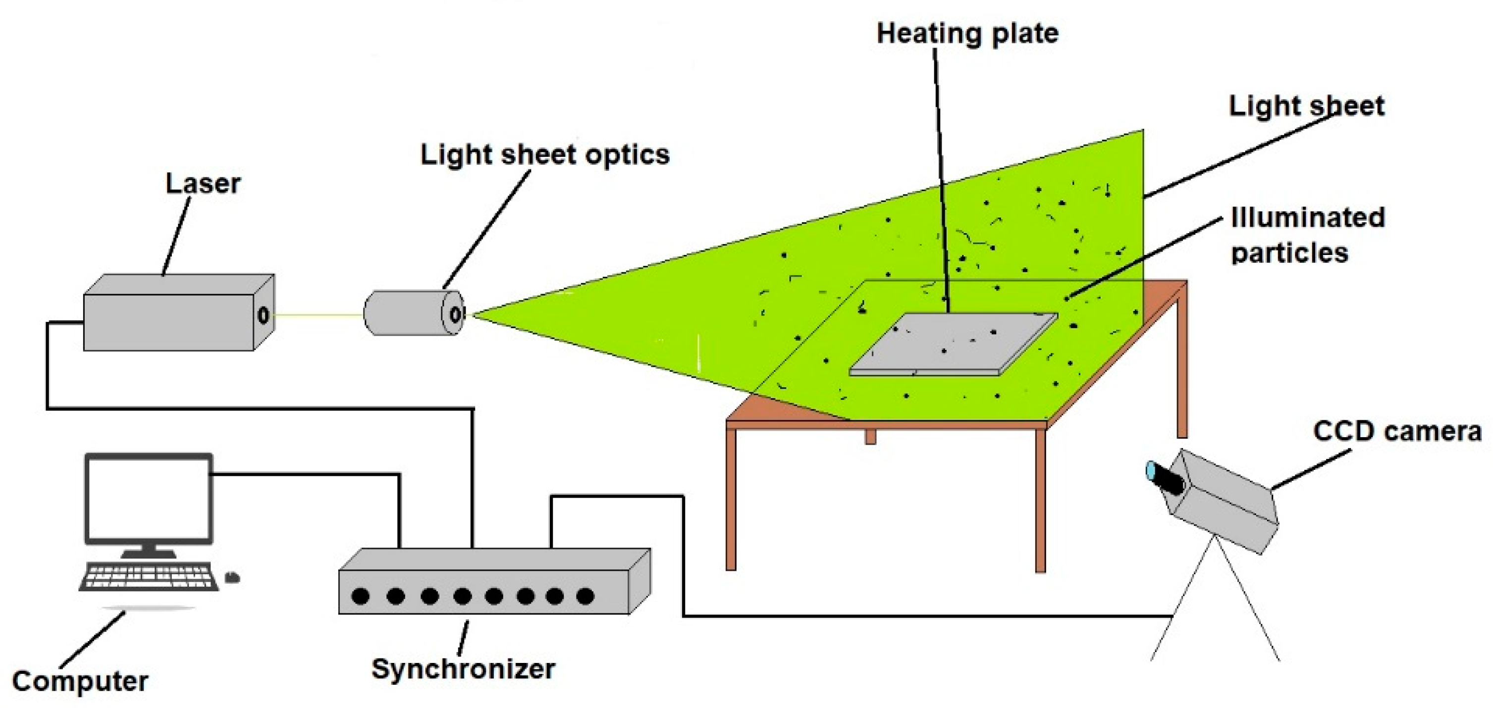
A laboratory experiment involved placing a heating foil on a worktable and creating a measuring plane around it using a high-powered laser with a wavelength of 532 nm, energy of 1200 mJ, and maximum power of 2000 W. The laser used was a two-chamber Nd: YAG pulsating laser CLASS 4. To capture the scattered light from tracer particles, a Flowsense EO high-speed CCD camera equipped with a matrix detector was used. The measuring plane was transformed into a light section by employing cylindrical optics. The FT700 CE particle generator from Dantec was used to create tracer particles in the form of oil droplets with sizes between 1 μm and 5 μm, using a maximum pressure of 4 bar and a volume of 4.5 l. However, the oil droplets alone were insufficient to capture the air flow around the heating foil in detail. To address this, a fog generator F2010 Plus was employed to create smaller particles (in size 1 μm) that provided more accurate information about the air flow.

The PIV technique involved taking images of the tracer particles’ starting and ending positions, which were analyzed using computer software to produce vector maps representing the velocity fields. The study utilized the PIV method to capture the flow of the fluid around the heating foil, which is demonstrated in Figure 2 of the research.

In summary, the laboratory experiment involved using the PIV method to measure the fluid flow around a heating foil. Tracer particles were produced with a particle generator and their motion was recorded using a high-speed CCD camera. The resulting images were analyzed with software to generate velocity maps of the fluid flow. For better visualization, a fog generator was employed to produce smaller particles. The PIV method process is illustrated in Figure 2.

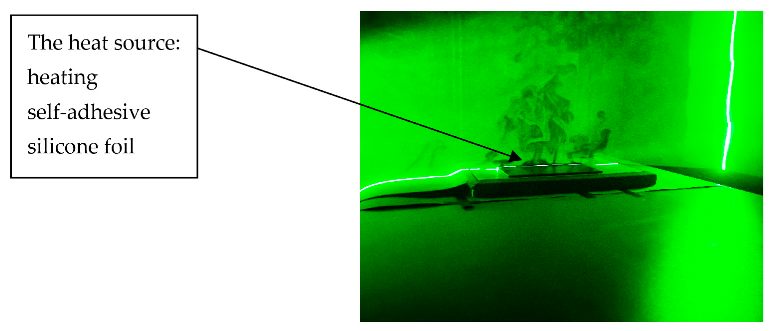
Figure 3 depicts the experimental setup, which includes a heating self-adhesive silicone foil (TF542) with specific dimensions (0.3 m × 0.2 m × 0.0013 m) and temperature capabilities—maximum temperature +200 °C. The foil generates a certain amount of power and affects the surrounding air flow through natural convection.

2.3. Data Processing

Data processing is a critical aspect of PIV analysis as it involves extracting meaningful information from the raw data obtained from the PIV experiment. The data processing steps involve various image processing, signal processing, and data analysis techniques to obtain accurate and reliable velocity measurements.

Before conducting any PIV experiments, it is necessary to perform a camera calibration to establish the scale between the object and image planes. In this study, the scale factor was determined, and 135 images were captured by CCD camera using the Image Run function within a very short time interval of 1000 µs, after successful calibration. To avoid measurement errors caused by the onset and closing of the laser, images that could have a large measurement error were filtered out [28,29].

Subsequently, the Image Masking function was then used to eliminate interfering elements and unnecessary areas from the images. In this experiment, a disturbing area from the bottom of the heating foil was removed because the foil had a glossy surface that reflected the laser beam.

The subsequent step in the procedure was to analyse and correlate the evaluation images using an adaptive correlation multi-stage algorithm based on cross-correlations. The investigation area was set at 64 × 64, with a Grid Step Size of 16 × 16 pixels. The Range Validation function was implemented to limit the size range of the vectors to be considered as accurate, within the speed range of 0 m·s⁻¹ to 0.5 m·s⁻¹. Vectors that did not fall within this range were removed from the evaluation. The Moving Average function was then applied to adjust the sizes of the vectors according to the neighbouring ones, creating a smooth velocity field without protruding vectors.

At the end of the evaluation, the Peak Validation function was used, setting a limit ratio of 1.2 px. The resulting vector field of air velocities after using the Peak Validation function is displayed in Figure 4.

Overall, data processing is a critical step in PIV analysis as it determines the accuracy and reliability of the velocity measurements. The quality of the PIV data can be improved by optimizing the processing parameters and using appropriate data filtering and smoothing techniques.

2.4. The Numerical Simulation of the Air Flow over the Heating Foil

The ANSYS Fluent software was used to perform a numerical simulation of the air flow around the heating foil in an open laboratory environment. The simulation involved a heating foil placed on a worktable, with length, width, and height dimensions of 300 mm, 200 mm, and 10 mm, respectively. The working fluid used in the simulation was air, and a simplified 3D model was employed.

The geometric parameters were inputted to create the 3D model in Design Modeler, which is depicted in Figure 5 and shows the model’s geometry and the surfaces under investigation. The dimensions of the model are presented in

Table 1. Dimensions of surfaces of model.

Dimensions	(m)
H9	0.300 m
L7	0.150 m
L6	0.150 m
V10	0.010 m
V8	0.500 m

.

In order to model heat transfer, particularly natural convection, a mesh was created and adapted for this purpose. The Inflation function was used to increase the number of cells around the heating foil’s surface, with cell sizes ranging from 0.001 m to 0.005 m and a total of 3,343,815 cells [30].

As the mathematical model in the ANSYS Fluent program was used a viscous model with laminar flow. This mathematical model is a commonly used model in ANSYS Fluent, a computational fluid dynamics software package. It is used to simulate the flow of a fluid that is both viscous and laminar. The viscous laminar model is generally suitable for simulating natural convection, which is the flow that occurs when a fluid is heated and rises due to buoyancy effects. In natural convection, the fluid flow is typically slow and laminar, which makes the viscous laminar model a good choice for simulating this type of flow. It is important to consider the specific characteristics of the flow being simulated and to choose the modelling approach that is best suited for the particular situation.

In this model, the fluid is assumed to be incompressible, and the flow is governed by the Navier-Stokes equations, which describe the motion of fluids. The model assumes that the flow is laminar, meaning that the fluid particles move in parallel layers without mixing or turbulence. This is in contrast to turbulent flow, which is characterized by chaotic, swirling motion.

The viscous laminar model also takes into account the viscosity of the fluid, which is a measure of its resistance to deformation. Viscosity is important in determining the amount of frictional forces between the layers of fluid, which in turn affects the overall flow behaviour.

Therefore, a laminar viscous model was chosen to simulate this type of solved problem, with using a Solver based on pressure with steady time and gravitational acceleration on the Y direction.

To use the viscous laminar model in ANSYS Fluent, it is typically needed to specify the properties of the fluid being simulated, such as its density, viscosity, and other relevant parameters. Very important is also to define the geometry of the simulation domain and set up appropriate boundary conditions to simulate the desired flow behaviour.

The equations that this mathematical model uses are:

• Continuity equation, which expresses the conservation of mass, stating that the rate of change of mass in any given volume of the fluid must be balanced by the rate of flow of mass into or out of that volume.

$$\nabla · \mathrm{v}=0$$

(2)

2.

Momentum equation, which expresses the conservation of momentum, stating that the rate of change of momentum of any given volume of the fluid must be balanced by the sum of the forces acting on that volume. The first term on the right-hand side represents the pressure gradient, which drives the fluid flow. The second term represents the viscous forces, which oppose the flow and are proportional to the rate of change of velocity with respect to distance.

$$\mathsf{\rho } · \left(\frac{\partial \mathrm{v}}{\partial \mathrm{t}}+\mathrm{v} · \nabla \mathrm{v}\right)=-\nabla \mathrm{p} + \mathsf{\mu }{\nabla }^2\mathrm{v}$$

(3)

Table 2. Material conditions.

Material	Density (kg×m−3)	Specific Heat (J×kg−1×K−1)	Thermal Conductivity (W×m−1×K−1)	Viscosity (kg×m−1×s−1)	Thermal Expansion Coefficient (K−1)
air	1.2047	1006.43	0.0242	sutherland	0.00343
aluminum	2719	871	202.4	−	−

,

Table 3. Boundary conditions.

		Set Parameters
Name	Type of Condition	Velocity (m·s−1)	Temperature (°C)
plate 1	No slip wall	0	124
plate 2	No slip wall	0	124
plate 3	No slip wall	0	124
Table 1	No slip wall	0	23.20
Table 2	No slip wall	0	23.20
output 1	Pressure-outlet	−	26.85
output 2	Pressure-outlet	−	26.85
output 3	Pressure-outlet	−	26.85

,

Table 4. Solution Methods.

Pressure-Velocity Coupling
Scheme	coupled
Spatial Discretization
Gradient	Green-Gauss Node Based
Pressure	Second Order
Momentum	Second Order Upwind
Energy	Second Order Upwind

,

Table 5. Solution controls.

Pseudo Transient Explicit Relaxation Factors
Pressure	0.5
Momentum	0.5
Density	1
Body Forces	1
Energy	0.75

and

Table 6. Run calculation.

Pseudo Transient Settings
Time step method	Automatic
Time scale factor	1
Length scale method	Conservative
Verbosity	0

provide details on the boundary, operational, material, and general condi-tions, as well as the set parameters and additional simulation settings.

The settings and inputs listed in the tables can be employed to conduct a numerical simulation of heat and mass transfer in an open space, using either a 2D or 3D model. In this particular case, the simulation was run for 500 iterations, but the boundary, material, and operational conditions can be modified to suit the specific characteristics of the system being modelled.

3. Results

To observe the airflow surrounding a heating foil, an experimental PIV (Particle Image Velocimetry) method was implemented. The approach involved using a high-speed camera to capture images of the light scattered from tracer particles within the fluid stream. The resulting images were subsequently analyzed using computer software to generate velocity maps along the entirety of the heating foil, pinpointing areas of peak velocity and temperature values of the airflow. The average temperature of the airflow was 26.85 °C, while the heating foil had 124 °C and the average air velocity was approximately 0.2 m·s⁻¹. These values were then used as inputs for a numerical simulation, which resulted in obtaining contours of temperature and airflow velocity for a 3D model of natural convection. 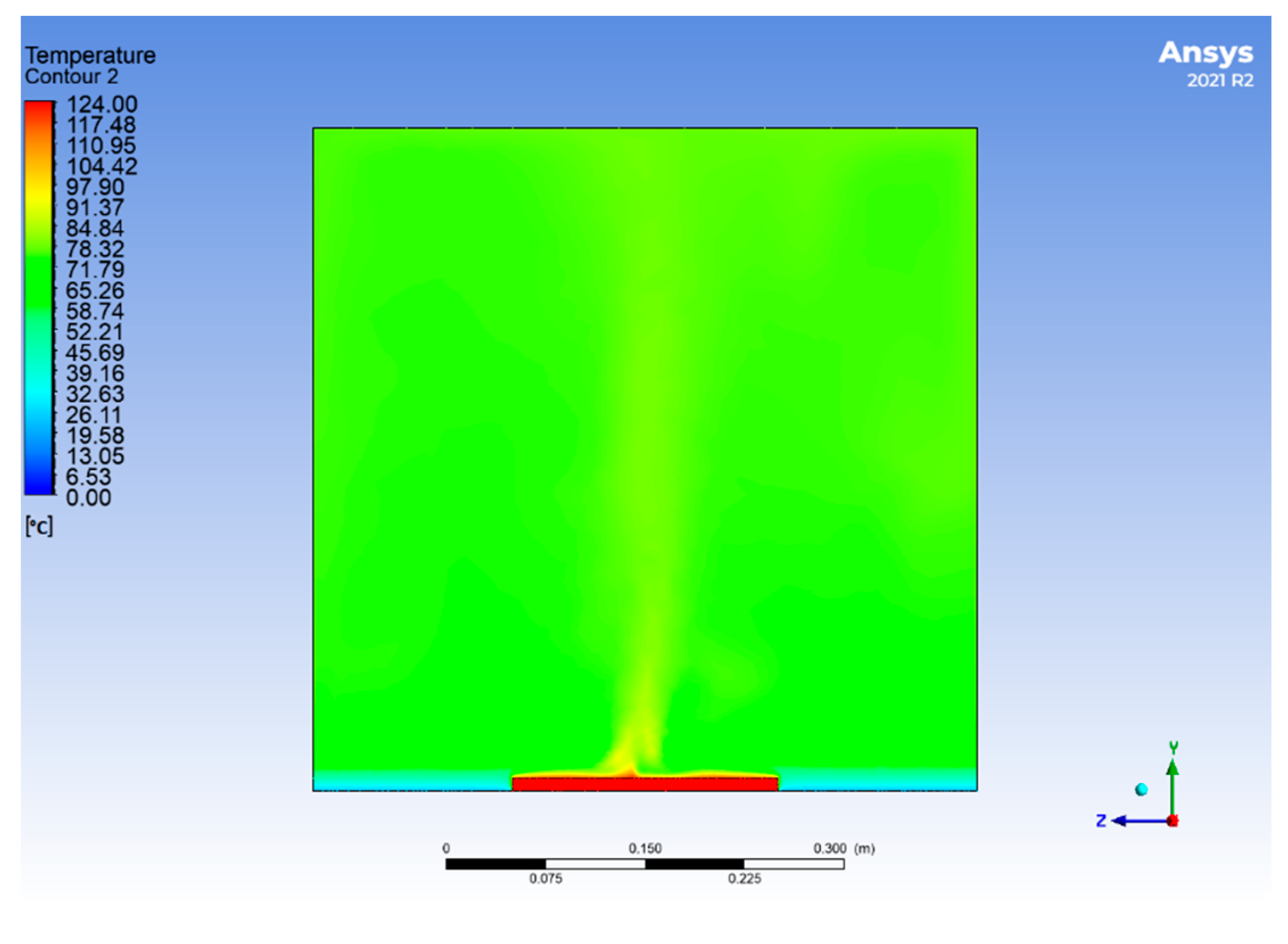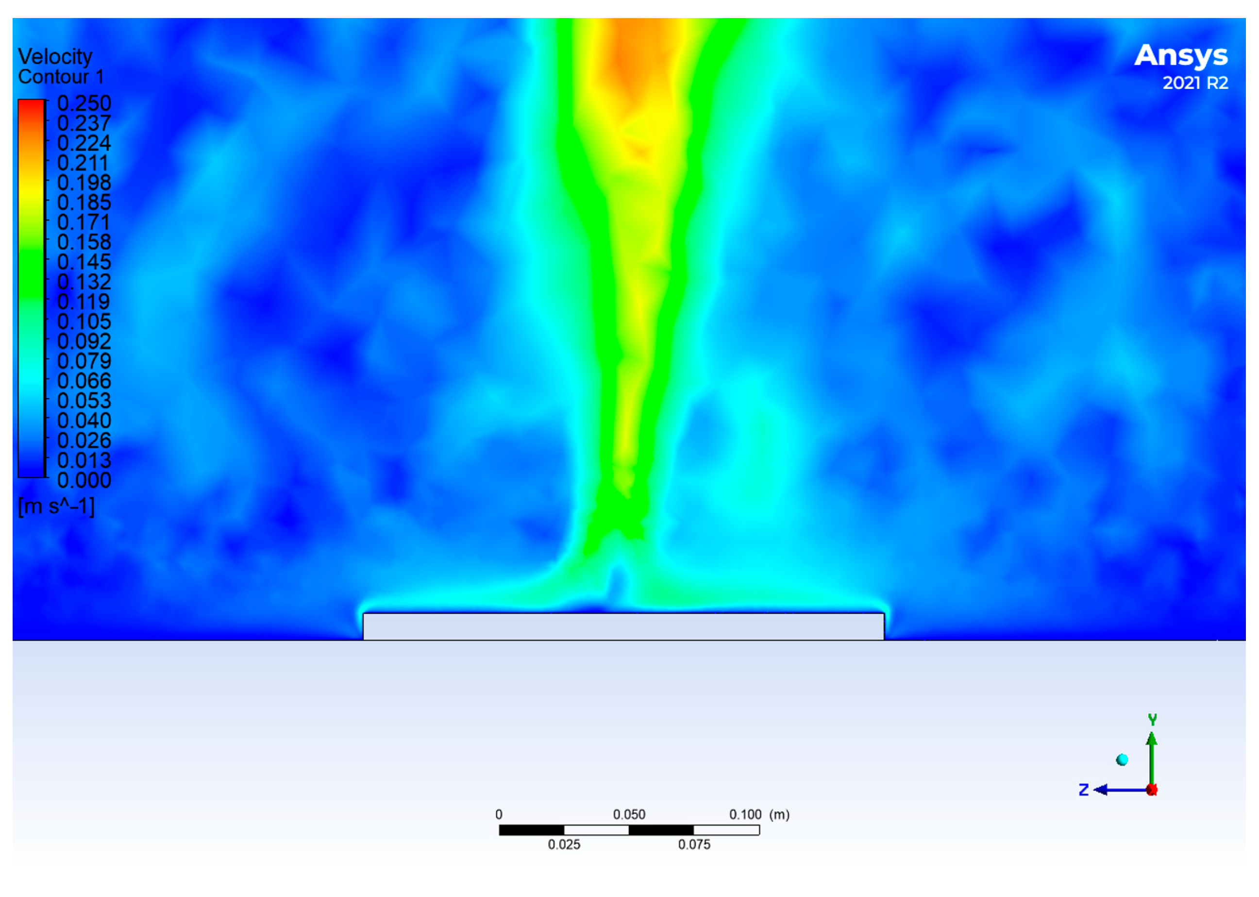Figure 6 shows the temperature contour, and Figure 7 shows the airflow velocity contour. The velocity contour demonstrates the creation of disturbing elements and air vortices due to the open space in the laboratory, which is expected in a real situation where there are other equipment influencing the heat transfer of the experiment. The details of these disturbing elements are shown in Figure 8.

The contours obtained from the numerical simulation show that the maximum temperature of 124 °C is on the surface of the heating foil, and the temperature gradually decreases with increasing distance from the surface until it stabilizes at the ambient air temperature of 26.85 °C. The velocity distribution map indicates that the airflow is stagnant at the top of the heating foil and in its immediate surroundings, but gradually gains speed as the distance from the surface of the heating foil increases. The highest velocity value obtained in this model is 0.250 m/s.

Straight lines were drawn on the images generated by the PIV method using an internal function, which allowed for the plotting of air velocities at predetermined heights above the surface of the heating foil. The straight lines were plotted at several distances above the surface of the heating foil in the range from 0.02 m to 0.4 m in different increments—0.02 m, 0.03 m, 0.04 m, 0.05 m, 0.06 m, 0.08 m, 0.1 m, 0.15 m, 0.2 m, 0.3 m, and 0.4 m.

According to natural convection theory, a boundary layer should exist which implies that there will be no velocity in the immediate vicinity above the heating foil. Figure 9 and Figure 10 exhibit the correlation between air velocity and particular heights above the heating foil’s entire surface.

Figure 11 illustrates a comparison between the velocity curves derived from experimental measurements using PIV and the CFD simulation, taken at a height of 150 mm above the heating foil surface. It is apparent that the experimental speeds reach lower values than the simulation, likely due to various external influences that are difficult to account for in a numerical model. These external factors can cause random phenomena that occur in a real environment but are difficult to predict in a simulated one. The maximum air velocities at this height are 0.1720 m·s⁻¹ in the CFD simulation, located in the middle of the plate, and 0.1614 m·s⁻¹ in the PIV measurement, with the peak shifting more towards the wall due to interfering elements.

The velocity of the air around a heating horizontal source due to natural convection depends on several factors, including the size and shape of the source, the temperature difference between the source and the surrounding fluid, and the properties of the fluid, such as its density, viscosity, and thermal conductivity.

In general, as the temperature of the source increases, the air around the source becomes less dense and rises, creating an upward flow of air. As this warm air rises, it creates a region of low pressure, which draws in cooler air from the surroundings to replace it. This cooler air is then heated by the source and rises in turn, creating a cycle of fluid motion.

The velocity of the air in this convection cell depends on the temperature difference between the source and the surrounding fluid, as well as the size and shape of the source. The velocity of the air can be calculated using equations derived from fluid mechanics, such as the Grashof number, which relates the buoyancy force to the viscosity and thermal diffusivity of the fluid. It is worth noting that the velocity of the air due to natural convection around a heating source is generally much lower than that due to forced convection, which is fluid flow that is driven by an external force, such as a fan or pump.

4. Conclusions and Discussion

This article discusses the visualization of airflow in the vicinity of a horizontal heating source subjected to natural convection in an open laboratory environment. Two methods were used to visualize the airflow: experimental Particle Image Velocimetry (PIV) and numerical simulation in Ansys Fluent. The velocity of air was the main parameter monitored in both methods. The experimental results were used as input data for the numerical simulation.

The simulation’s findings indicated the existence of air swirls and disruptive components. These were recognized by charting the correlation between air speed across the whole heating foil at specific elevations above it. Additionally, the simulation recorded the speed boundary layer near the heating foil, with the highest air velocities situated in the middle of the heating foil.

To sum up, the successful visualization of airflow was accomplished by utilizing both PIV and numerical simulation methods. The implementation of PIV allowed for the detection of air vortices and other environmental issues, while numerical simulation enabled the optimization of the airflow. Additionally, by modifying the input data, the 3D model of natural convection over the horizontal heating foil to open space of the laboratory can be used for similar simulations by changing the input data.

The visualization results are important for achieving optimal parameters, such as the output of the heater and the heating source temperature, which affect the thermal comfort in the interior and ensure comfort for the user. The results can also help in better understanding the vorticity of flow in the environment and prevent disturbing elements that create this vorticity. The research was influenced by many external factors, which would also need to be tested at different values. The vision would be the creation of a calibration graph in which the dependences of the performance of such internal heating sources on external parameters would be plotted, so that the thermal comfort would be achieved through the proper calibration. The presence of air vortices together with dust from surrounding areas can cause discomfort in the workplace and human health problems. Therefore, this visualization can contribute to improving the overall environment quality and well-being of the occupants.