Biomimetic and Constructal Design of Alveolus-Inspired Extended Surfaces for Heat Dispersion

Abstract

Biomimetics is a school of design based on taking inspiration from nature to solve complex problems. This is done with the assumption that the natural world already has solutions to many engineering problems that have been refined through trial and error—an example of the constructal law. In this study, biomimicry is used to investigate the impact of the shape of an extended surface for mixed convection cooling within the context of the cavity problem. This is a simplified two-dimensional case that aims to develop new heat dispersal ideas for use in electronics, power generation, and industrial applications. A numerical model is developed and solved using ANSYS Fluent and the results were examined for varying Reynolds, Rayleigh, and Richardson numbers with the goal of maximizing heat transfer. The results show that the alveolus-inspired fin design provides better heat transfer compared with the design based on a rectangular fin in a cavity.

1. Introduction

Convective heat transfer is one of the most studied research areas in mechanical engineering due to its wide range of practical applications both in industry and consumer electronics, from race car radiators to solar panels to mobile devices—virtually any technology dealing with heat needs some way to disperse it and so there is great interest in maximizing the efficiency of the heat transfer in these systems. Various scenarios have been investigated previously, from the simple square cavity with a rectangular fin [1,2,3,4,5,6,7,8], to more geometrically complex cases [9,10,11,12,13,14,15,16] to investigations into the effects of less common conductive mediums such as nanofluids [6,7,17,18] and non-Newtonian fluids [19]. As this area is so widely studied, there is a great breadth of variety in the literature: studies like Starner et al. [1] investigated free-convection from rectangular-fin arrays, Mahmud et al. [2,11] studied wavy cavities and the orientations of a square cylinder, Ting et al. [7] highlighted the impact of surface roughness in a square cavity, Aziz [20] investigated the effects of different fin shapes, Szodrai [21] investigated heat sink shape for a hypothetical scenario, where air cooling is needed and to save energy the pressure loss and the cooling performance have to be equally optimized, while some like Tari and Mehrtash [22] focused on how heat transfer can be affected by various boundary configurations with respect to gravity, and others explored the consequences of using a porous fin [23].

Many of these investigations were guided by the constructal law, coined by Adrian Bejan in 1996 [24], which attempts to describe the requirements for a physical system to persist in time. These include investigations by Rodrigues et al. [8] studying the effects of a double fin setup, Lorenzini et al. [16] into cross-shaped and T-shaped convection fins, Cong et al. [6] studying the constructal design of rectangular fins, and Razera et al. [25] into elliptical fins, which all help provide a more complete understanding of the physical phenomena governing cavity heat transfer and fin optimization. In addition, Nemati and Ardekani [26] proposed a new method called natural construction inspired by the constructal law, and Dirker and Meyer [27] highlighted the design of internal solid-state conductive systems using topology optimization.

Another method used to try and maximize heat transfer is biomimicry. Biomimetics is a design method that involves taking inspiration from natural systems and features to find efficient and effective solutions to complex problems and has been used for a variety of applications from aircraft wing design to structural coloration. The biomimetic design was utilized in the lid-driven cavity by Kobayashi et al. [15] and Calamas and Baker [14] when they investigated the consequences of imitating the fractal nature of trees in their extended surface designs and has led to improve the development of biomimetic alveoli structure capsules that have been found to increase the thermal response of heat storage units [24]. Biomimicry is especially powerful as it allows us to apply designs already tested and iterated upon by nature that we may not have thought of to problems they are particularly suited to solving. As the constructal law seemingly governs evolution in living creatures [28] it is often found that biomimetic solutions represent ‘local maxima’, that is to say, they offer optimal solutions given limited resources [29].

This study attempted to combine these two design methods to investigate the impact of the fin geometry within the lid-driven cavity problem under mixed convection conditions. Natural convection is a result of the inherent heterogeneity in the fluid; hotter material is less dense and so rises, creating an area of lower pressure that colder matter moves into, resulting in a net flow of fluid. Forced convection, on the other hand, is caused by an external force that drives the particles. For a given system to be classified as mixed convection, the natural and forced convection must be of a similar magnitude [30]. In this case, neither dominates the interaction, making the analysis tricky due to the complex interaction between buoyancy and the shear force.

In this study, the inspiration for the extended surfaces investigated was based on mammalian alveoli, small air sacs in the lungs where blood exchanges oxygen and carbon dioxide to facilitate respiration, as shown in Figure 1. A side effect of this process is that water diffuses into the lungs and is exhaled, taking with it heat from the body and playing a key part in thermal regulation. For some mammals, evaporative heat loss is the primary source of heat dissipation and panting is vital for keeping cool on hot days or after exercise [31]. As the lung structure is optimized for heat exchange [32] and acts as a mass transfer device, it was decided to attempt to recreate this in the lid-driven cavity problem. Therefore, an attempt was made to examine the effects of alveoli-inspired fins in the two-dimensional lid-driven cavity under mixed convection in water with a constant-temperature fin in an attempt to investigate the effect of fin geometry for maximizing heat transfer.

2. Methodology

The constructal design method is used to obtain an optimal geometry, one which allows the maximum heat transfer between the thermal medium and the extended surface. To this end, several fin geometries were investigated, starting with a basic rectangular fin and gradually approximating the alveolar shape. In this study, the fin area was held constant and the height, length and, if applicable, radii, are considered the degrees of freedom of the system. Several values of the Rayleigh (Ra) and Reynolds (Re) numbers were examined to evaluate the corresponding temperature and flow fields as well as heat transfer for each fin to evaluate an optimal geometry.

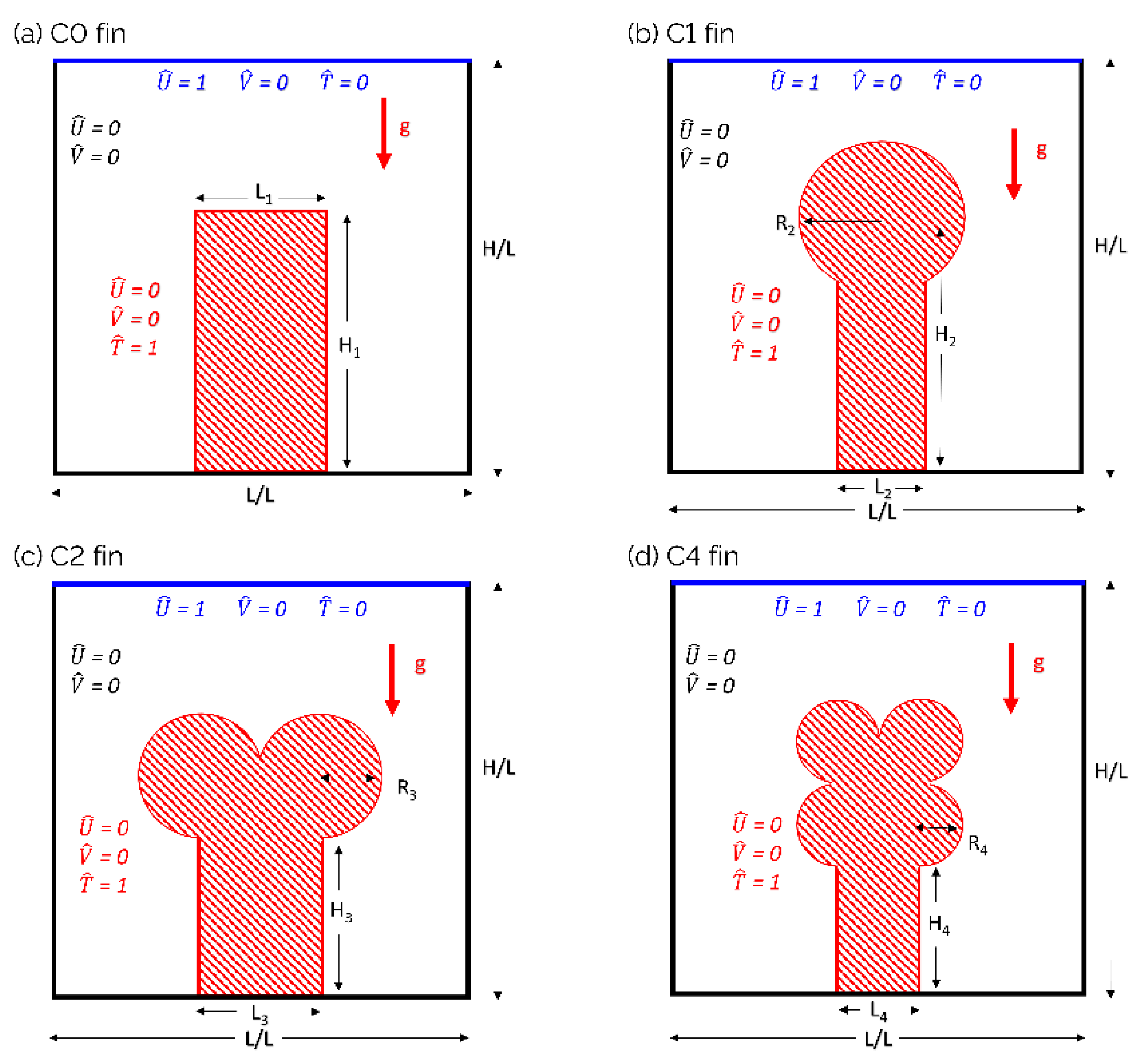
2.1. Problem Description

We considered a lid-driven square cavity with a fin from the center of the bottom. This geometry includes symmetrical boundary conditions on the left and right walls. The top surface of our cavity has a constant temperature $T_{\min }$ and moves with constant velocity $U_{\max }$ in the x-axis direction, providing both the temperature differential necessary to drive the natural convection and the external force required to drive the forced convection. The fin surface has a constant wall temperature $T_{\max }$. The dimensionless height and length of the cavity are both set to 1, and the fin area is set to 20% of the cavity area. All other surfaces are considered adiabatic, and the no-slip condition is applied. Figure 2 shows the specific geometries tested. For the C0 fin, the height-to-length ratio was chosen to be 2 which gave L₁ = 1/√10 and H₁ = 2/√10. For the alveolus fins, two cases were considered: (i) the radius of the alveolar sacs is equal to the width of the fin base (Figure 2b), and (ii) the radius of the alveolar sacs is half to the width of the fin base (Figure 2c,d). The side length (L₂) and radius (R₂) of the C1 fin was chosen to be 0.2, which led to H₂ = 0.650. For the C2 fin, the radii were chosen to be 0.15, which constrained the length to 0.3 and resulted in a height of 0.380. Finally, the radii of the C4 fin’s circles were set to 0.1 giving a length of 0.2 and a height of 0.307.

The dimensionless velocities ($\widehat{U}$ and $\widehat{V}$) and temperature ($\widehat{T}$) included in Figure 2 are defined as:

$$\widehat{U}=\frac{u}{U_{\max }}$$

(1)

$$\widehat{V}=\frac{v}{U_{\max }}$$

(2)

$$\widehat{T}=\frac{T-T_{\min }}{T_{\max }-T_{\min }}$$

(3)

2.2. Governing Equations

This system is governed by the conservation of energy, mass, and momentum described by the Navier–Stokes equations for a two-dimensional laminar mixed convective flow. As we have a fluid of variable temperature and therefore density, and the difference in inertia is negligible compared to gravity, it is convenient for us to apply the Boussinesq approximation in the y-direction as the change in temperature is small therefore the change in density is much smaller than the reference density. This greatly simplifies the problem and makes the simulation much less computationally intensive. Therefore, the governing equations are written as [6,7]:

$$\mathrm{Continuity}: \frac{\partial u}{\partial x}+\frac{\partial v}{\partial y}=0$$

(4)

$$x\mathrm{-Momentum}: u\frac{\partial u}{\partial x}+v\frac{\partial u}{\partial y}=-\frac{1}{\rho }\frac{\partial p}{\partial x}+\frac{\mu }{\rho }\left(\frac{{\partial }^{2}u}{\partial x^2}+\frac{{\partial }^{2}u}{\partial y^2}\right)$$

(5)

$$y\mathrm{-Momentum}: u\frac{\partial v}{\partial x}+v\frac{\partial v}{\partial y}=-\frac{1}{\rho }\frac{\partial p}{\partial y}+\frac{\mu }{\rho }\left(\frac{{\partial }^{2}v}{\partial x^2}+\frac{{\partial }^{2}v}{\partial y^2}\right)+g\beta \left(T-T_{\infty }\right)$$

(6)

$$\mathrm{Energy}: u\frac{\partial T}{\partial x}+v\frac{\partial T}{\partial y}=\frac{k}{\rho C_p}\left(\frac{{\partial }^{2}T}{\partial x^2}+\frac{{\partial }^{2}T}{\partial y^2}\right)$$

(7)

where u and v are the horizontal and vertical velocities, p is the pressure, μ is the dynamic viscosity, ρ is the density, β is the thermal expansion coefficient, T is the temperature, g is the standard gravity, k is the heat conductivity, and C_p is the heat capacity.

3. Numerical Modeling

3.1. Dimensionless Variables and Simulation Cases

In mixed convection, the two means of heat dispersion can be quantified for easier comparison using the dimensionless Rayleigh (Ra) and Reynolds (Re) numbers, and they can be calculated with the following expressions:

$$\mathrm{Re}=\frac{\rho H{U}_{\max }}{\mu }$$

(8)

$$\mathrm{Ra}=\frac{g\beta \Delta T{L}^3}{\nu \alpha }$$

(9)

Each fin was therefore simulated for differing Reynolds and Rayleigh numbers in order to determine the effect of different kinds of flows with varying buoyancy and inertial forces on the heat transfer of each fin. The number of simulations to be run is [No. of Re tested] × [No. of Ra tested] × [number of fins] which can grow rapidly so to choose the number of values of Re and Ra tried a decision was weighed about quality against time restraints. Once these simulations were run it was possible for us to plot the simulations of differing Re, Ra, and fin shapes to identify the best choice for each. It will also be useful later to compare the Richardson numbers (Ri) of each fin and flow to visualize how buoyancy affects and drives each flow:

$$\mathrm{Ri}=\frac{\mathrm{Ra}}{{\mathrm{Re}}^2\mathrm{Pr}}$$

(10)

where Pr is the Prandtl number, the ratio of kinematic viscosity to the thermal diffusivity:

$$\mathrm{Pr}=\frac{\nu }{\alpha }$$

(11)

3.2. Grid Size Determination

The governing partial differential equations were solved numerically using the built-in SIMPLE pressure-based solver of ANSYS Fluent, with the second-order upwind scheme used to spatially discretize the equations. The solution was considered converged when the residuals were smaller than 10⁻⁶ for the mass and momentum equations and smaller than 10⁻⁸ for the energy equation. After a solution was calculated, the average Nusselt number (Nu_avg) was found using the following expression [6,7]:

$${\mathrm{Nu}}_{\mathrm{avg}}=\frac{1}{S}{\displaystyle {\int }_s^{}{\mathrm{Nu}}_{\mathrm{H}} \mathrm{d}S}=\frac{1}{S}{\displaystyle {\int }_s^{}\frac{h_{nf}H}{k_{nf}}\mathrm{d}S}$$

(12)

where S is the fin surface and h is the heat transfer coefficient of the thermal interface. The area-weighted average Nusselt number is a dimensionless quantity that expresses the heat transfer of a fluid as a ratio of the convective and conductive components, with a larger number denoting greater convection. A higher Nusselt number is more desirable as it indicates a greater convection component, while we expect the conduction component to be largely similar, with differences mainly caused by increasing surface area, but this also increases the convection component. Therefore, this study is concerned with optimizing the average Nusselt number. This number can also be used to run a grid independence test to compare the accuracy of different grid sizes to determine a suitable grid size by considering the desired level of accuracy. This was necessary to ensure the simulation results were not affected by the resolution of the grid whilst also minimizing computation time.

It was decided to use triangular meshes for this problem as, although quadrilateral meshes are considered to be more accurate than triangles in more complex calculations, due to the triangular cell only having three vertices and sides whereas the quadrilateral cell shape has four of each, it was concluded that this could be made up for with a finer grid of triangles to achieve the desired level of accuracy. Moreover, as this is a relatively simple physical problem with more complex geometry, triangular meshes were believed to be sufficient in this scenario.

The mesh sensitivity test was run for grids of 60 × 60, 80 × 80, 100 × 100, 120 × 120, 140 × 140 and 160 × 160 cells for each fin type, with simulation parameters Ra = 10⁵, Re = 10³_, and the results are shown in Figure 3. When increasing the mesh size, we expect to see the average Nusselt number increase as it approaches the true value. As can be seen from Figure 3a, the average Nusselt number value is getting closer to its true value with the increase in mesh size. Above mesh sizes of 100 × 100 there is very little difference between the average Nusselt number for each mesh therefore any mesh above this size could be considered good enough for our purposes. It was also observed that each of the meshes took a fairly similar amount of time for a solution to become converged, with greater mesh sizes taking a small amount longer than previous smaller ones, except the 160 × 160 mesh which took noticeably longer to compute.

A similar pattern was observed for each mesh so to aid in the mesh selection. The percentage of error in the average Nusselt number is calculated for each mesh to compare each mesh’s accuracy. This was based on the idea that a finer mesh will produce a more accurate result therefore percentage accuracy was calculated based on the Nusselt number of the current mesh and the previous mesh. Figure 3b shows the percentage error for each of the mesh resolutions tested for each fin at Ra = 10⁵ and Re = 10³. An acceptable percentage error value was chosen to be less than 0.5%, which for each fin is achieved by the 120 × 120 mesh. This, along with the similar computation time led to the decision to run further simulations with this size mesh for each fin.

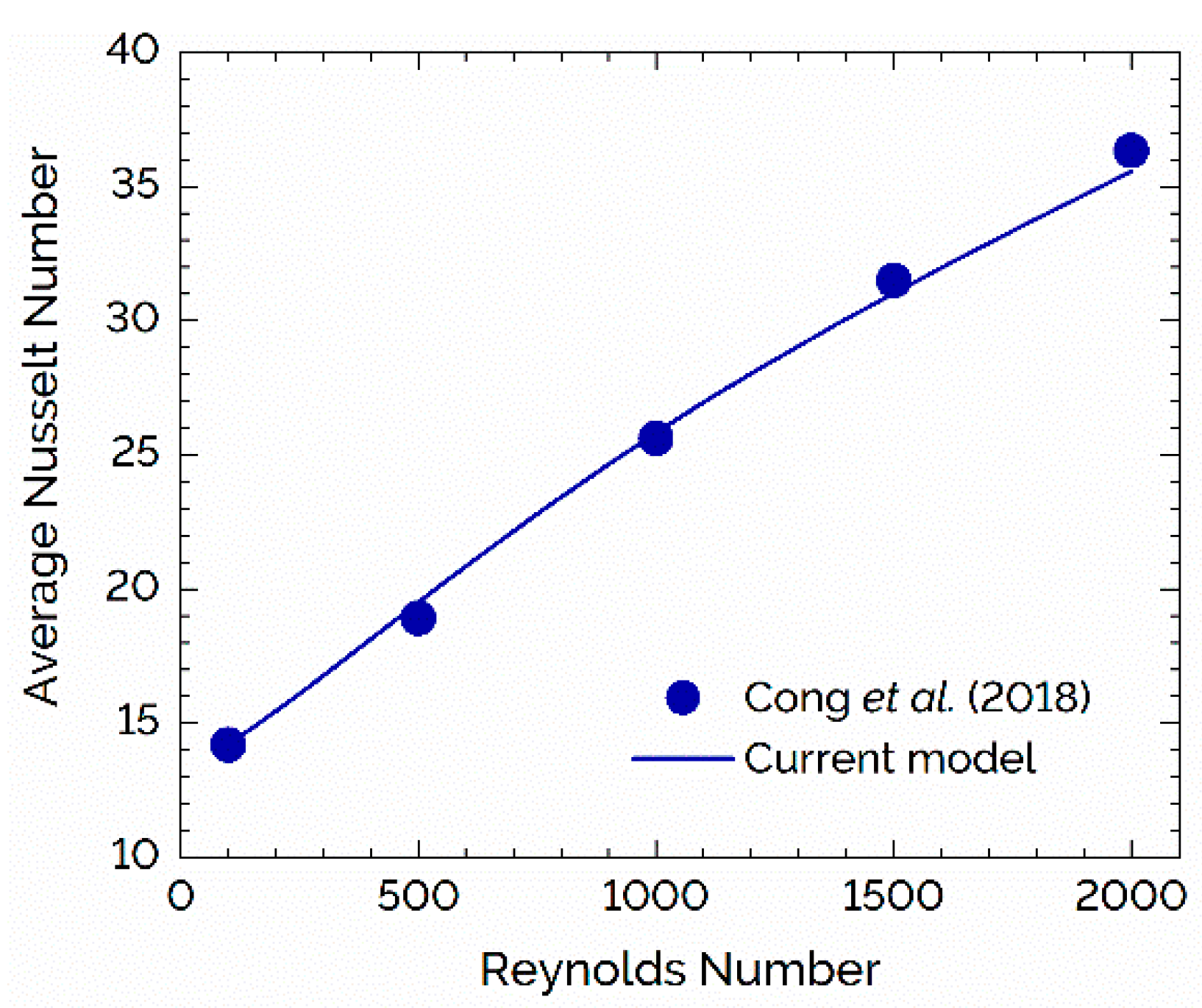
3.3. Model Validation

To be confident in the validity of the created model, it was necessary to recreate a previous investigation and verify that the results obtained matched this benchmarked data. This is because without validation there is a significant risk of user error in the model that will lead to results that are not truly representative of the physical processes simulated, and therefore jeopardizing the integrity of the study. To this end, a simplified geometry was modeled, as the geometry considered in this study is not currently represented in the available literature. A mixed convection flow in a cavity of Al₂O₃-water nanofluid with intruded by a rectangular fin with H₁/L₁ = 0.5, H₁/L₁ = 0.05, and T = T_max was analyzed so that the benchmark results of Cong et al. [6] could be used for comparison. Otherwise, the setup, assumptions, and governing equations are the same as described above, with the fin surrounded by adiabatic no-slip walls, the top surface with a temperature of T_min and moving in the positive x-direction with velocity U_max, and gravity acting downwards with acceleration g.

In order to recreate this investigation, it was necessary to calculate the thermo-physical properties of the fluid used in the prior study. For this, the Brinkman model [33] was used to calculate the dynamic viscosity of the fluid, the Maxwell model [34,35] was used to calculate the effective thermal conductivity, and the density, the specific heat capacity, and thermal expansion were calculated using classical mixing theory, as these approaches are widely used in various applications [35,36,37].

$$\mathrm{Effective} \mathrm{density}: {\rho }_{nf}=(1-\varphi ){\rho }_f+\varphi {\rho }_s$$

(13)

$$\mathrm{Thermal} \mathrm{expansion} \mathrm{coefficient}: {\beta }_{nf}=\frac{(1-\varphi ){\rho }_f{\beta }_f+\varphi {\rho }_s{\beta }_s}{{\rho }_{nf}}$$

(14)

$$\mathrm{Heat} \mathrm{capacity}: C_{p,nf}=\frac{(1-\varphi ){\rho }_f{C}_{p,f}+\varphi {\rho }_s{C}_{p,s}}{{\rho }_{nf}}$$

(15)

$$\mathrm{Dynamic} \mathrm{viscosity}: {\mu }_{nf}=\frac{{\mu }_f}{{(1-\varphi )}^{2.5}}$$

(16)

$$\mathrm{Thermal} \mathrm{conductivity}: k_{nf}=\frac{k_f\left(k_s+2k_f-2\varphi (k_f-k_s)\right)}{k_s+2k_f+\varphi (k_f-k_s)}$$

(17)

where the subscripts nf refers to the properties of the nanofluid, s refers to Al₂O₃ nanoparticles and f refers to water, φ is the fraction of nanoparticles suspended in the particle by volume, and all other parameters are the same as defined earlier. Thermo-physical properties of water and Al₂O₃ nanoparticles used in this study are listed in

Table 1. Thermo-physical properties of water and Al₂O₃ nanoparticles [6].

Physical Property	Water	Al2O3	Unit
Dynamic viscosity (µ)	1 × 10−3	-	kg⋅m−1
Density (ρ)	997.1	3970	kg⋅m−3
Thermal expansion (β)	2.1 × 10−4	8.5 × 10−6	K−1
Heat conductivity (k)	0.613	40	W⋅m−1K−1
Heat capacity (Cp)	4179	765	J⋅kg−1K−1
Kinematic viscosity (ν)	1.005 × 10−6	-	m2⋅s−1
Thermal diffusivity (α)	1.471 × 10−7	-	m2⋅s−1

.

With these properties calculated, simulations could now be run for a Rayleigh number of 10⁵ and varying Reynolds numbers to compare the current model to the expected results. As can be seen in Figure 4, the results calculated closely match the benchmark data and so we can now be confident of the conclusions we draw from further investigations. In addition to validation shown in Figure 4, Figure 5a shows one of the results this test was trying to emulate whilst Figure 5b is the result obtained from the present work. While these are not completely identical, the similarities are greater than the small differences. This might be more concerning had the average Nusselt number not been close to the target value therefore this simulation was considered accurate enough for our purposes.

4. Results and Analysis

4.1. Effects of Reynolds Number

After running simulations for each fin with varying Reynolds and Rayleigh numbers, the results were collated so the effects could be compared. Figure 6a shows the variation in the average Nusselt number for the rectangular fin (C0 fin) as these parameters change, and it can be seen that increasing either the Reynolds or Rayleigh numbers results in an increased average Nusselt number, showing greater convective heat transfer under these conditions. The graph also clearly shows that for smaller values of Rayleigh number (≤10⁴) there is little difference in average Nusselt number between orders of magnitude however as the Rayleigh number increases it begins to dominate the flow at Reynolds numbers below 500. This is indicative of the natural convection requiring a minimum threshold before it begins to meaningfully contribute to the heat dispersion. Moreover, as the Reynolds number increases it can be seen that the average Nusselt numbers calculated for each value of the Rayleigh number get closer together, illustrating how the flows become less and less buoyancy-driven, as the forced convection begins to dominate. It may also be noted that for lower Rayleigh numbers there appears to be a linear relationship between the Reynolds number and the average Nusselt number however this relationship becomes more quadratic as the Rayleigh number increases.

The results for the alveolar fin (C1 fin) given in Figure 6b follow a similar trend to those found for the rectangular fin at a low Reynolds number, with a slightly higher average Nusselt number in each case, however, it can be seen immediately that for a high Rayleigh number the trend is quite different, with the average Nusselt number leveling out for Reynolds numbers higher than 500. This is surprising and at first, seems to be some kind of error in the calculation as the Nusselt number hits a peak at Re = 500 however even if this data point is erroneous, it does not account for the relatively shallow gradient between Re = 750 and Re = 1000. Another explanation for this plateau is that with such strong gravitational forces and a fin geometry that gives a lot of room for vortexes to form the forcing velocity at which heat dissipation is maximized is low enough that increasing it further does little to increase the flow rate past the fin and therefore the cooling capacity of the cavity. This creates a limit on how much heat can be removed from the fin due to the motion of the top edge and means the average Nusselt number stagnates. It can also be seen that this geometry results in the Ra = 10⁵ case being much more similar to the simulations with smaller Raleigh numbers than in the previous geometry. Similarly, to the rectangular fin, the convergence of Nusselt number at higher Reynolds numbers indicates that here the forced convection is the main contributor to the heat dissipation and the natural convection’s contribution is less relevant with increasing forcing, a result that will hold for the other two fin geometries tested.

4.2. Effects of Increasing Rayleigh Number

Figure 7 depicts the contours of static temperature for the C2 fin under different Rayleigh numbers to illustrate how the fin is affected. As can be seen, when the gravity of the simulation increases it causes a more dramatic flow of cold water to the bottom of the cavity which results in a current visible in flow fields (Figure 8). This current brings more cool water from the top surface to the fin and so allows for a more efficient transfer of heat. This effect is minor at first however for larger Raleigh numbers it has a substantial impact on the system, eventually creating a pocket of cool water on the right of the fin that allows for a continuous supply of heat transfer from the fin. The effect can more clearly be seen in Figure 8, which shows velocity contours for the fin with varying Rayleigh numbers. Here, the convection currents caused by the downward flow of dense cold fluid are apparent and it can be seen that at first the flow of water only travels past the top of the fin however as the acceleration due to gravity increases (and therefore the difference in downwards force between hot and cold air increases) more liquid is dragged past the fin’s surface and is available to carry heat away from the fin. This effect is visible in all four fins (see Figure 9 and Figure 10), with roughly the same magnitude however the greatest flow is from the rectangular fin as it does not have any protrusions that constrict the flow of a fluid like the other fins.

Figure 8 faintly shows a slow-moving convection current below the main current for the fin with Ra = 10⁵ that helps disperse heat from the right side of the fin and it can be seen that as the Rayleigh number increases this develops into a much quicker stream that combines with the main current to send fast-moving liquid across the right of the fin allowing for much greater cooling. The Ra = 10⁶ fin also has a faint current forming on the left side of the fin however due to the forcing velocity on the top surface it is much harder for this current to form, even with a relatively low Reynolds number. If the fin’s area were not such a large fraction of the cavity it is possible, we would see more convection on the left side of the fin however the fin acts as a barrier both between the left and right of the cavity and also to a lesser extent the top and bottom due to the circles protruding from the top of the fin.

The heat from each of the fins is trapped on the left of the fins, showing how powerful the cooling effect of the convection current is. We can see that the C0 and C2 fins have a more heterogeneous spread of heat contours directly above the fins than the C1 or C4 fin and this is caused by the greater vertical space between the wall and the fin allowing a wider channel of fluid through and so allowing a greater spread of heat.

The velocity contours for each fin at this high Rayleigh number are very similar so there is evidence to suggest that the effect of the geometries chosen have a minimal effect on the fluid flow formed. A far greater variable appears to be the distance of each fin from the top wall as this is where there is greater variation in velocities, with the right two fins showing a smaller stream of high-speed fluid.

4.3. Effects of Increasing Reynolds Number

Figure 11 and Figure 12 show the contours of static temperature and velocity contours for the C1 fin for varying Reynolds numbers to help visualize the effect this has on the flow. Figure 11 shows that as the Reynolds number increases there is an expansion of the area the cool fluid takes up implying better heat dissipation and there is also the expansion of mid-temperature range zones shown in green. This represents the increased mixing of air allowing heat to leave the fin that is caused by an increase in the forcing velocity however it can be seen that there is not as much difference in the cases of Re = 750 and Re = 1000 compared to the difference between Re = 500 and Re = 750 which may point to the cavity reaching the limit of forcing velocity before faster fluid flow does not improve the heat transfer.

Looking at Figure 12 we can see how increasing the Reynolds number causes a buildup of fast-moving fluid in the top right of the cavity, leading to increased heat transfer in this area and driving the convection of the water. It is notable that the increased velocity at higher Reynolds numbers appears to have only increased the flow velocity in the top right, whereas over the rest of the fin it appears the velocity has either stagnated or decreased. Due to this, the effects of increasing the top wall velocity do not seem to change much between the geometries tried as despite their different shapes the current appears to be largely the same. Again, this may be due to the fin’s area being such a large fraction of the cavity that there is not enough room for the vortex to fully form and preventing the flow of liquid from integrating fully. In future experiments, it would be prudent to vary area fraction in order to see the effects of this on the different types of fins.

When comparing how the Reynolds number affects the different geometries Figure 13 shows us that the forcing velocity causes the fluid flow to be very similar in all cases. This explains why in the graphs shown in Figure 6 there is greater unity of average Nusselt number for higher Reynolds numbers; for large forcing velocities the fins act very similarly despite different gravitational accelerations as the flow is dictated by the Reynolds number which as we can see leads to a persistent pattern of fluid flow, thus resulting in a predictable Nusselt number varying only slightly due to gravity. It is worth noting that it appears as though the fin that traps the least heat is the standard fin as there does not seem to be as much hot air pooling on the left side of the cavity. This is only a minor effect, but, interestingly, the more complex geometries create stagnant areas for heat to pool.

One of the reasons for the differing geometries resulting in the same flow pattern is that they are all fairly tall compared to the cavity and all split the space in two. It is therefore worth conjecturing that if either the area fraction or aspect ratios of the fins were different whether the same pattern would be observed. It looks as though for all the fins there are various degrees of flow separation, with the C2 and C4 fins being more notable as it appears to be trapping heat in the top surfaces of the fins rather than letting it dissipate (Figure 14).

4.4. Effects of Richardson Number

Using the relation defined in Equation (10), the Richardson number for differing Reynolds numbers could be calculated to analyze how buoyancy affects the fluid flow. Figure 15a shows how the average Nusselt number varies with the Richardson number for the C4 fin for several Reynolds numbers. A Richardson number of approximately 1 predicts that the flow will be buoyancy-driven and we can see that for each of the Reynolds numbers the average Nusselt number begins to rise rapidly at around this value, showing the considerable heat dissipation power of moving from forced to mixed convection. It can be seen that for values less than 1, the average Nusselt number is approximately constant showing that the heat transfer under purely forced convection is much weaker than the mixed convection at higher Ri.

Figure 15b shows how the Richardson number changes for the different fins and we can see that they are all extremely similar, displaying the same pattern, with the main difference being the magnitude of the Nusselt number calculated. It can be seen that mixed convection begins at around Ri = 0.1 for each of the fins as expected and before this the average Nusselt number is steady. This is consistent with Figure 8 which does not begin to show clear signs of mixed convection until after Ra = 10⁵ which corresponds to Ri = 0.058.

This graph clearly shows that for all values of Ra and Re numbers, the C1 fin has the best rate of thermal transport, followed by the C4 and C2 fins. It is not surprising that the basic rectangular fin fared worst as it has the smallest surface area and therefore less contact area to disperse heat however it is surprising how close the bottom two fins were. The C2 fin has almost 25% more surface area than the rectangular fin yet it does not seem to be much better at losing heat. Moreover, the C1 fin has less surface area than both the C2 and C4 fins but is much at dispersing heat and this may be because the latter two have a nook where the circles meet which can trap hot fluid and this is shielded from the convection current. The C1 fin on the other hand is smooth the whole way around and its circle meets the ‘stem’ at an obtuse angle meaning it is much easier for air to move past it. This leads to much better heat transfer as more cool water gets to the surface of the fin and becomes available to transmit heat.

5. Conclusions

This study has developed a numerical model to analyze a lid-driven cavity with various fins and investigate the mixed convection of various alveolus-inspired heat-exchange fins with the goal of finding an optimum geometry for heat dissipation in water. The thermal properties of these fins were examined under varying Reynolds, Rayleigh, and Richardson numbers. This led to the conclusion that for maximum heat transfer, the most important factor is geometry which highlights the unrestricted movement of fluid through the cavity, as any areas where fluid can get stuck lead to an inefficient buildup of heat that can negatively impact the heat dispersion. It was also found that although it can be beneficial, fin perimeter does not necessarily correlate with effective heat transfer and so optimizing for this is not the best option when designing exterior fins. This study has found that a rectangular intruded fin can be improved by adding a bulbous head to the end to increase surface area however care must be taken to ensure surfaces meet at obtuse angles to prevent the buildup of the hot medium. Furthermore, it has been interpreted that increasing the Rayleigh number of the system can vastly increase the rate of heat loss if there is sufficient space for a convection current to form that can take cool fluid to the fin and away again. Likewise, a high Reynolds number was found to be beneficial to heat loss however it appeared as though at low Rayleigh numbers a high Reynolds number preferred lots of space between the top surface and the fin, as the C1 fin appeared to suffer from reduced flow compared to the shorter fin. Looking forward, it would be useful to investigate how Reynolds number would affect the fins differently if they had a smaller area fraction and so there was more room for the fluid to flow. Another idea would be to see how changing the proportions of the fins might affect their heat dissipation and if removing the crevices from some of the fins allows the medium to flow around them more easily. It may also be prudent to see how these fins are affected by nanofluids and if there would be a stronger correlation between perimeter and Nusselt number with a more thermally conductive medium.

References

1. Starner, K.E.; McManus, H.N., Jr. An experimental investigation of free-convection heat transfer from rectangular-fin arrays. J. Heat Transf. 1963, 85, 273–277. [Google Scholar] [CrossRef]
2. Mahmud, S.; Das, P.K.; Hyder, N. Laminar natural convection around an isothermal square cylinder at different orientations. Int. Commun. Heat Mass Transf. 2002, 29, 993–1003. [Google Scholar] [CrossRef]
3. Harahap, F.; Rudianto, E.; Pradnyana, I.G.D.M.E. Measurements of steady-state heat dissipation from miniaturized horizontally-based straight rectangular fin arrays. Heat Mass Transf. 2005, 41, 280–288. [Google Scholar] [CrossRef]
4. Shi, X.; Khodadadi, J.M. Laminar fluid flow and heat transfer in a lid-driven cavity due to a thin fin. J. Heat Transf. 2002, 124, 1056–1063. [Google Scholar] [CrossRef]
5. Lorenzini, G.; Estrada, E.D.D.; dos Santos, E.D.; Isoldi, L.A.; Rocha, L.A.O. Constructal design of convective cavities inserted into a cylindrical solid body for cooling. Int. J. Heat Mass Transf. 2015, 83, 75–83. [Google Scholar] [CrossRef]
6. Cong, R.; Ozaki, Y.; Machado, B.S.; Das, P.K. Constructal design of a rectangular fin in a mixed convective confined environment. Inventions 2018, 3, 27. [Google Scholar] [CrossRef] [Green Version]
7. Ting, K.; Mozumder, A.K.; Das, P.K. Effect of surface roughness on heat transfer and entropy generation of mixed convection in nanofluid. Phys. Fluids 2019, 31, 093602. [Google Scholar] [CrossRef]
8. Rodrigues, P.M.; Biserni, C.; de Escobar, C.C.; Rocha, L.A.O.; Isoldi, L.A.; dos Santos, E.D. Geometric optimization of a lid-driven cavity with two rectangular intrusions under mixed convection heat transfer: A numerical investigation motivated by constructal design. Int. Commun. Heat Mass Transf. 2020, 117, 104759. [Google Scholar] [CrossRef]
9. Das, P.K.; Mahmud, S. Effect of eccentricity and radius ratio on fluid flow and heat transfer inside an eccentric semicircular enclosure. J. Therm. Sci. 2000, 9, 135–140. [Google Scholar] [CrossRef]
10. Tasnim, S.H.; Mahmud, S.; Das, P.K. Effect of aspect ratio and eccentricity on heat transfer from a cylinder in a cavity. Int. J. Numer. Methods Heat Fluid Flow 2002, 12, 855–869. [Google Scholar] [CrossRef]
11. Mahmud, S.; Das, P.K.; Hyder, N.; Islam, A.K.M.S. Free convection in an enclosure with vertical wavy walls. Int. J. Therm. Sci. 2002, 41, 440–446. [Google Scholar] [CrossRef]
12. Das, P.K.; Mahmud, S. Numerical investigation of natural convection inside a wavy enclosure. Int. J. Therm. Sci. 2003, 42, 397–406. [Google Scholar] [CrossRef]
13. Das, P.K.; Mahmud, S.; Tasnim, S.H.; Islam, A.K.M.S. Effect of surface waviness and aspect ratio on heat transfer inside a wavy enclosure. Int. J. Numer. Methods Heat Fluid Flow 2003, 13, 1097–1122. [Google Scholar] [CrossRef] [Green Version]
14. Calamas, D.; Baker, J. Tree-like branching fins: Performance and natural convective heat transfer behavior. Int. J. Heat Mass Transf. 2013, 62, 350–361. [Google Scholar] [CrossRef]
15. Kobayashi, H.; Lorente, S.; Anderson, R.; Bejan, A. Trees and serpentines in a conducting body. Int. J. Heat Mass Tran. 2013, 56, 488–494. [Google Scholar] [CrossRef]
16. Lorenzini, G.; Medici, M.; Rocha, L.A.O. Convective analysis of constructal t-shaped fins. J. Eng. Thermophys. 2014, 23, 98–104. [Google Scholar] [CrossRef]
17. Zhao, W.; Mozumder, A.K.; Das, P.K. Mixed convection of CuO-water nanofluid in a square enclosure with an intruded rectangular fin. AIP Conf. Proc. 2018, 1980, 050004. [Google Scholar]
18. Hussain, S.; Jamal, M.; Geridonmez, B.P. Impact of fins and inclined magnetic field in double lid-driven cavity with Cu–water nanofluid. Int. J. Therm. Sci. 2021, 161, 106707. [Google Scholar] [CrossRef]
19. Rot, M.; Kosec, G. Natural convection of non-newtonian fluids in a differentially heated closed cavity. In Proceedings of the 2021 44th International Convention on Information, Communication and Electronic Technology (MIPRO), Opatija, Croatia, 27 September–1 October 2021; pp. 259–264. [Google Scholar]
20. Aziz, A. Optimum dimensions of extended surfaces operating in a convective environment. Appl. Mech. Rev. 1992, 45, 155–173. [Google Scholar] [CrossRef]
21. Szodrai, F. Heat sink shape and topology optimization with pareto-vector length optimization for air cooling. Energies 2020, 13, 1661. [Google Scholar] [CrossRef] [Green Version]
22. Tari, I.; Mehrtash, M. Natural convection heat transfer from inclined plate-fin heat sinks. Int. J. Heat Mass Transf. 2013, 56, 574–593. [Google Scholar] [CrossRef]
23. Wang, L.; Wang, W.-W.; Cai, Y.; Liu, D.; Zhao, F.-Y. Effects of porous fins on mixed convection and heat transfer mechanics in lid-driven cavities: Full numerical modeling and parametric simulations. Transp. Porous Media 2020, 132, 495–534. [Google Scholar] [CrossRef]
24. Bejan, A. Street network theory of organization in nature. J. Adv. Transp. 1996, 30, 85–107. [Google Scholar] [CrossRef]
25. Razera, A.L.; da Fonseca, R.J.C.; Isoldi, L.A.; dos Santos, E.D.; Rocha, L.A.O.; Biserni, C. Constructal design of a semi-elliptical fin inserted in a lid-driven square cavity with mixed convection. Int. J. Heat Mass Transf. 2018, 126, 81–94. [Google Scholar] [CrossRef]
26. Nemati, H.; Ardekani, M.M. Heat sink evolutionary optimization by natural construction method. Numer. Heat Transf. Part A: Appl. 2021, 80, 168–183. [Google Scholar] [CrossRef]
27. Dirker, J.; Meyer, J.P. Topology optimization for an internal heat-conduction cooling scheme in a square domain for high heat flux applications. J. Heat Transf. 2013, 135, 111010. [Google Scholar] [CrossRef]
28. Bejan, A.; Lorente, S. The constructal law and the evolution of design in nature. Phys. Life Rev. 2011, 8, 209–240. [Google Scholar] [CrossRef] [PubMed]
29. Rogers, J.S.; Swofford, D.L. Multiple local maxima for likelihoods of phylogenetic trees: A simulation study. Mol. Biol. Evol. 1999, 16, 1079–1085. [Google Scholar] [CrossRef] [Green Version]
30. Basak, T.; Roy, S.; Sharma, P.K.; Pop, I. Analysis of mixed convection flows within a square cavity with uniform and non-uniform heating of bottom wall. Int. J. Therm. Sci. 2009, 48, 891–912. [Google Scholar] [CrossRef]
31. Robertshaw, D. Mechanisms for the control of respiratory evaporative heat loss in panting animals. J. Appl. Physiol. 2006, 101, 664–668. [Google Scholar] [CrossRef]
32. Knudsen, L.; Ochs, M. The micromechanics of lung alveoli: Structure and function of surfactant and tissue components. Histochem. Cell Biol. 2018, 150, 661–676. [Google Scholar] [CrossRef] [PubMed]
33. Brinkman, H.C. The viscosity of concentrated suspensions and solutions. J. Chem. Phys. 1952, 20, 571. [Google Scholar] [CrossRef]
34. Garnett, J.C.M. Colours in metal glasses and in metallic films. Philos. Trans. R. Soc. London. Ser. A Contain. Pap. A Math. Or Phys. Character 1904, 203, 385–420. [Google Scholar] [CrossRef] [Green Version]
35. Das, P.K.; Li, X.; Liu, Z.S. Effective transport coefficients in PEM fuel cell catalyst and gas diffusion layers: Beyond Bruggeman approximation. Appl. Energy 2010, 87, 2785–2796. [Google Scholar] [CrossRef]
36. Das, P.K.; Li, X.; Liu, Z.S. Analytical approach to polymer electrolyte membrane fuel cell performance and optimization. J. Electroanal. Chem. 2007, 604, 72–90. [Google Scholar] [CrossRef]
37. Weber, A.Z.; Borup, R.L.; Darling, R.M.; Das, P.K.; Dursch, T.J.; Gu, W.B.; Harvey, D.; Kusoglu, A.; Litster, S.; Mench, M.M.; et al. A critical review of modeling transport phenomena in polymer-electrolyte fuel cells. J. Electrochem. Soc. 2014, 161, F1254–F1299. [Google Scholar] [CrossRef]
Figure 1. A depiction of human alveoli, bronchioles, and blood vessels facilitating gas exchange. Here, the alveoli are analogous to our fin and the blood vessels are analogous to the thermal medium. Image credit: https://en.wikipedia.org/wiki/Pulmonary_alveolus (accessed on 16 October 2022).
Energies 16 00066 g001
Figure 2. Diagram of the lid-driven cavity intruded by a constant temperature fin. (a) rectangular fin (C0), (b) fin with one facsimile alveolus (C1), (c) fin with two facsimile alveoli (C2), (d) fin with four facsimile alveoli (C4). Here, the fin area is fixed (Afin = 0.2) with respect to the cavity area in all cases.
Energies 16 00066 g002
Figure 3. (a) The results of the mesh test for the C1 fin with Ra = 105 and Re = 103. Here, the number of mesh elements is plotted against the average Nusselt number for each size showing the convergence to the true answer as the mesh becomes finer. (b) The percentage error in each mesh size for each fin geometry (as shown in Figure 2).
Energies 16 00066 g003
Figure 4. Results from simulations using the current model overlaid onto benchmark results from Cong et al. [6].
Energies 16 00066 g004
Figure 5. Contours of temperature at Re = 500, Ra = 105 for Al2O3-water nanofluid: (a) Cong et al. [6] and (b) result from the current model with the same configuration of Cong et al. [6].
Energies 16 00066 g005
Figure 6. Effect of varying Rayleigh and Reynolds numbers on the rectangular fin (C0 fin) and alveolar fin (C1 fin).
Energies 16 00066 g006
Figure 7. Temperature contours for the C2 fin with Re = 100 for varying Rayleigh numbers. From left to right, top to bottom: Ra = 103, Ra = 104, Ra = 105, and Ra = 106.
Energies 16 00066 g007
Figure 8. Velocity contours for the C2 fin with Re = 100 for varying Rayleigh numbers. From left to right, top to bottom: Ra = 103, Ra = 104, Ra = 105, and Ra = 106.
Energies 16 00066 g008
Figure 9. Thermal contours for each of the fins at Re = 100 and Ra = 106, showing how strong gravity leads to a less even temperature spread.
Energies 16 00066 g009
Figure 10. Velocity contours for each of the fins at Re = 100 and Ra = 106, illustrating the convection currents formed due to the difference in density between hot and cold fluid.
Energies 16 00066 g010
Figure 11. Temperature contours for the C1 fin with Ra = 103 for varying Raynolds numbers. From left to right, top to bottom: Re = 100, Re = 500, Re = 750, and Re = 1000.
Energies 16 00066 g011
Figure 12. Velocity contours for the C1 fin with Ra = 103 for varying Raynolds numbers. From left to right, top to bottom: Re = 100, Re = 500, Re = 750, and Re = 1000.
Energies 16 00066 g012
Figure 13. Thermal contours for each of the fins at Re = 1000 and Ra = 103, showing the impact of increased top edge velocity.
Energies 16 00066 g013
Figure 14. Velocity contours for each of the fins at Re = 1000 and Ra = 103, showing how each fin’s geometry affects fluid flow with a large forcing velocity.
Energies 16 00066 g014
Figure 15. (a) Average Nusselt number against Richardson number for the C4 alveolar fin, and (b) average Nusselt number against Richardson number for each fin with Re = 500.
Energies 16 00066 g015