
Experimentally Validated Modelling of an Oscillating Diaphragm Compressor for Chemisorption Energy Technology Applications

Abstract
:1. Introduction
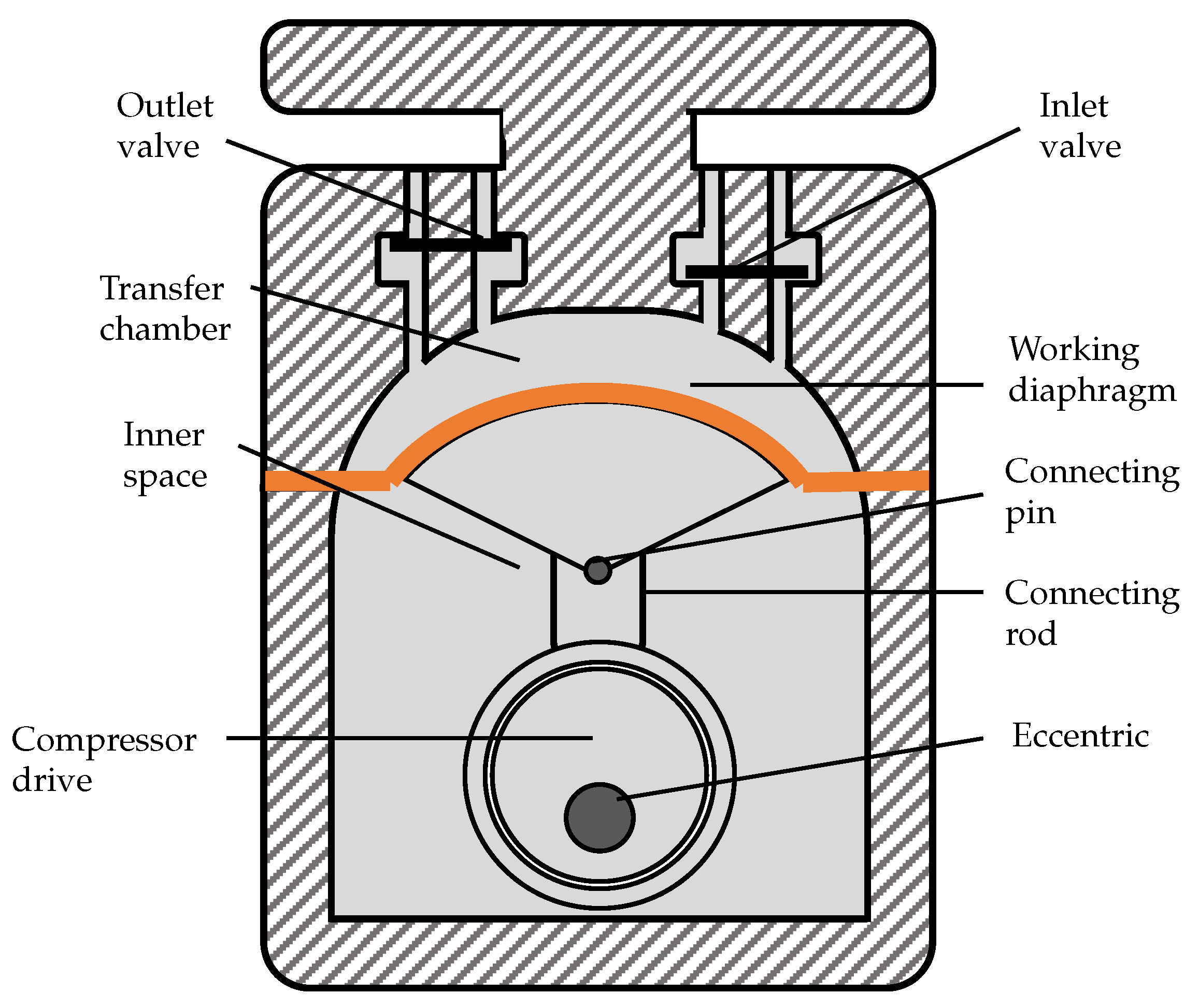
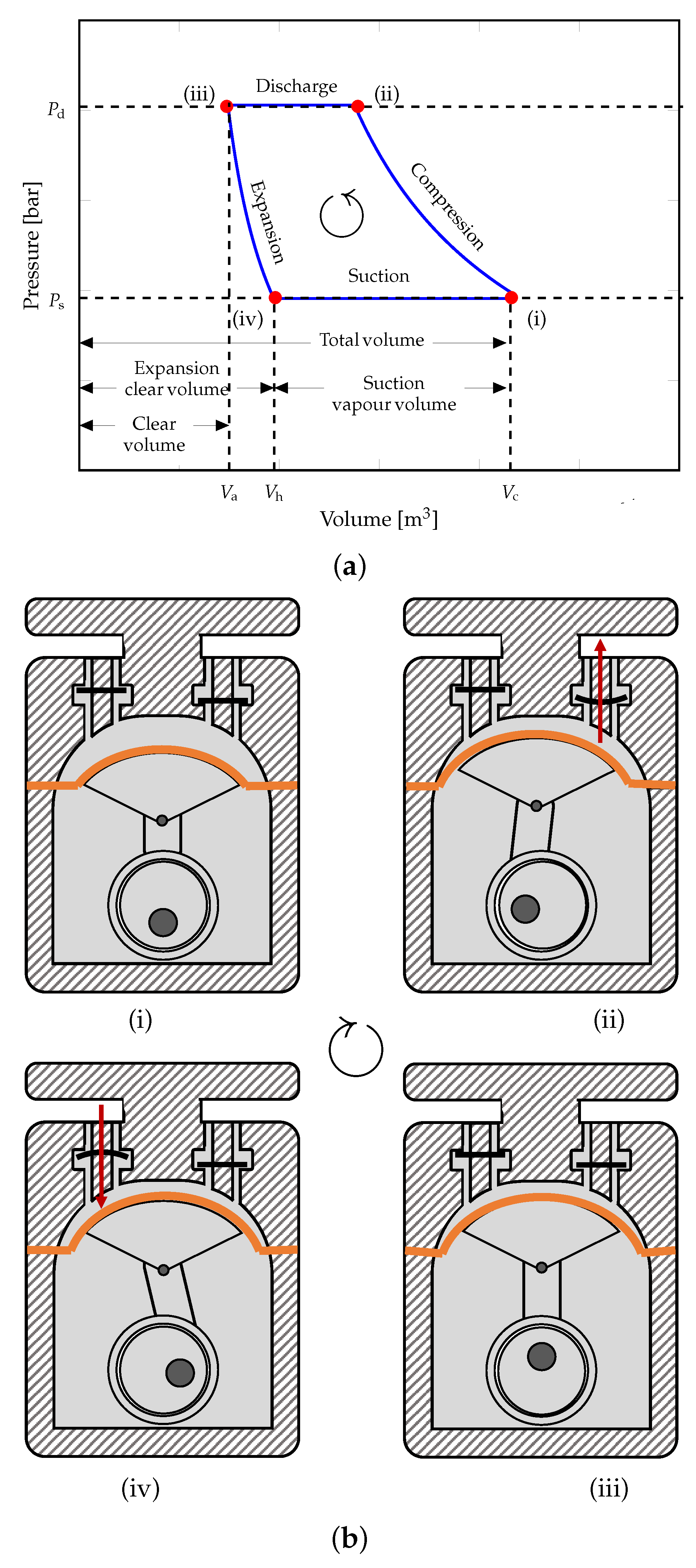
2. Diaphragm Compressor Working Principals
3. Model Development
3.1. Geometry Description of Diaphragm Compressor
3.2. Thermodynamics Modelling
3.3. Modelling Algorithm
- The gas leakage through the reed valve is negligible;
- The rotation speed of the compressor is initially pre-defined at a fixed value;
- The pressure drop through the reed valve is pre-defined at a fixed value, therefore the gas pressure has no change during suction and discharge stages;
- Gas is uniformly distributed inside the compressor;
- The pre-defined rotational speed is used to determine the time interval and rotational angel at present calculation step;
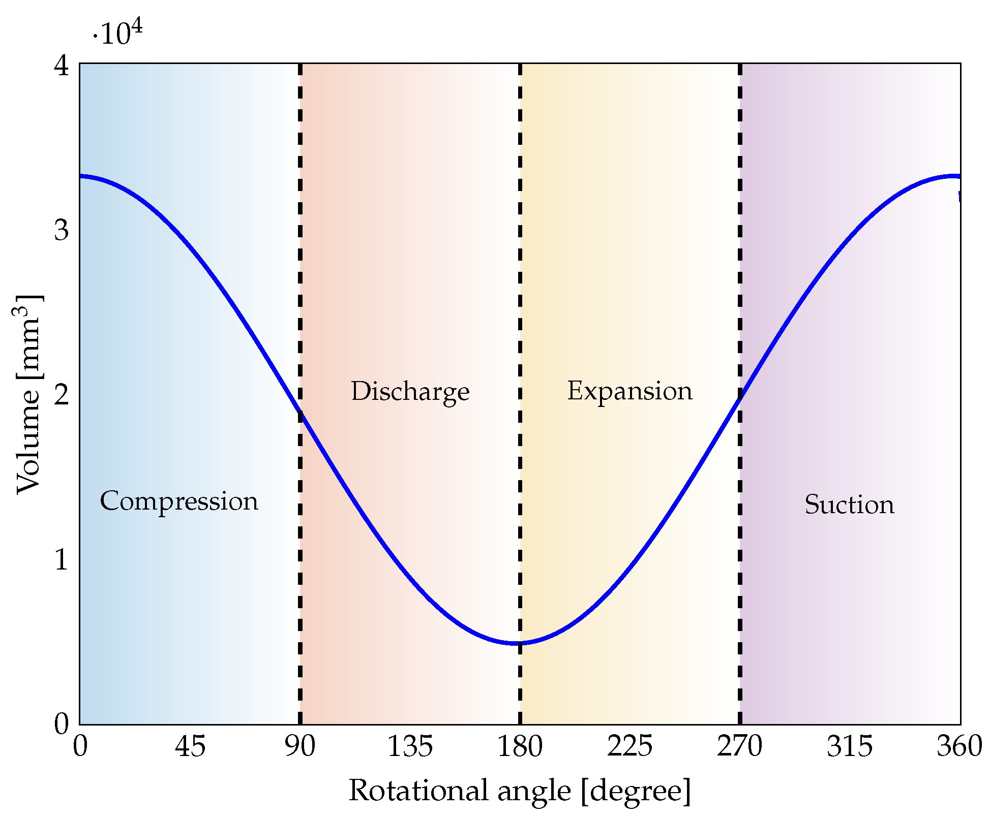
- The present rotational angel is used to determine the present volume;
- The present rotational angel and previous gas pressure are used to determine which stage of the process among compression, discharge, expansion and suction;
- The thermodynamic equation and heat transfer equation are called to calculate the present gas pressure, temperature and other properties;
- The mass flow rates in suction and discharge stages are determined based on the assumed constant gas pressure caused by the assumption of fixed pressure drop through reed valves.
- The time step is 0.0005 s to make sure that all the short-timescale dynamic effects are captured in the model, and the process is modelled for 20 s.
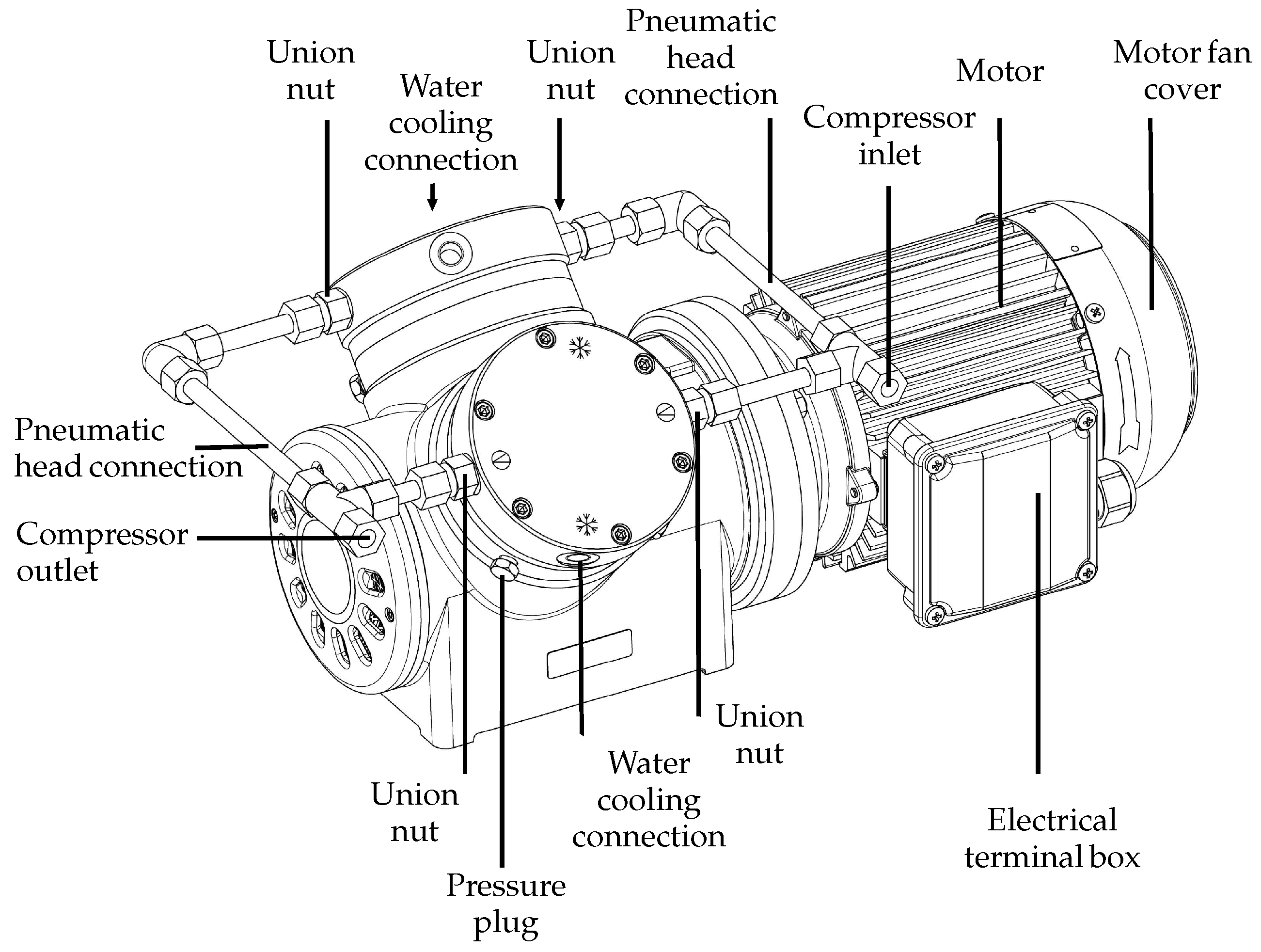
4. Experimental Apparatus
5. Results and Discussion
5.1. Model Validation
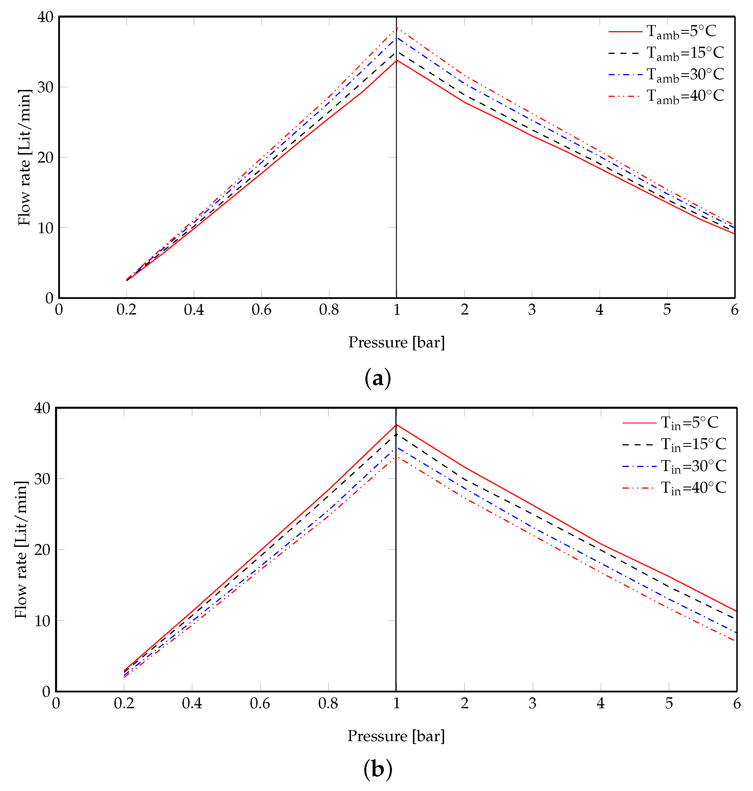
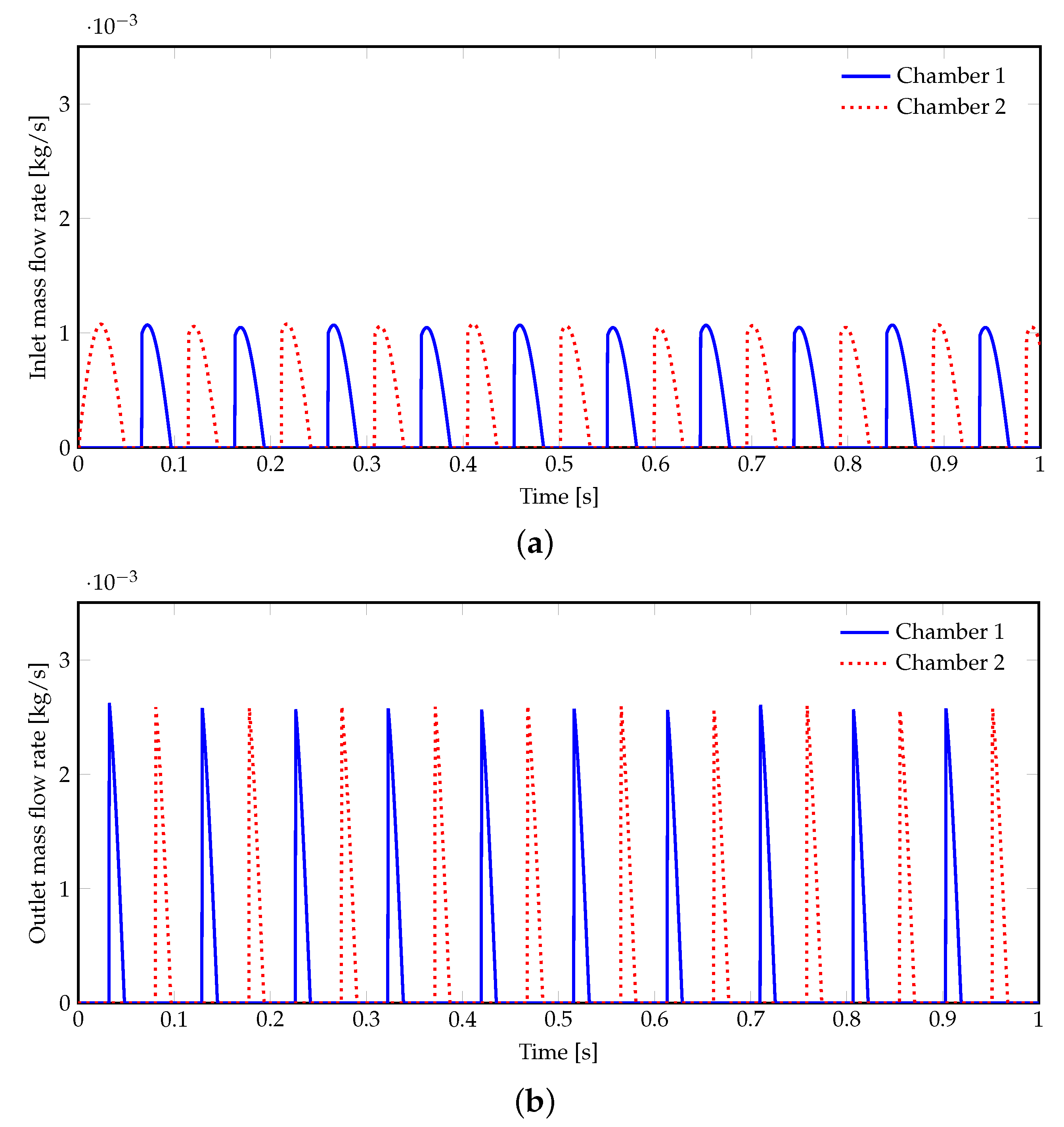
5.2. Flow Rate
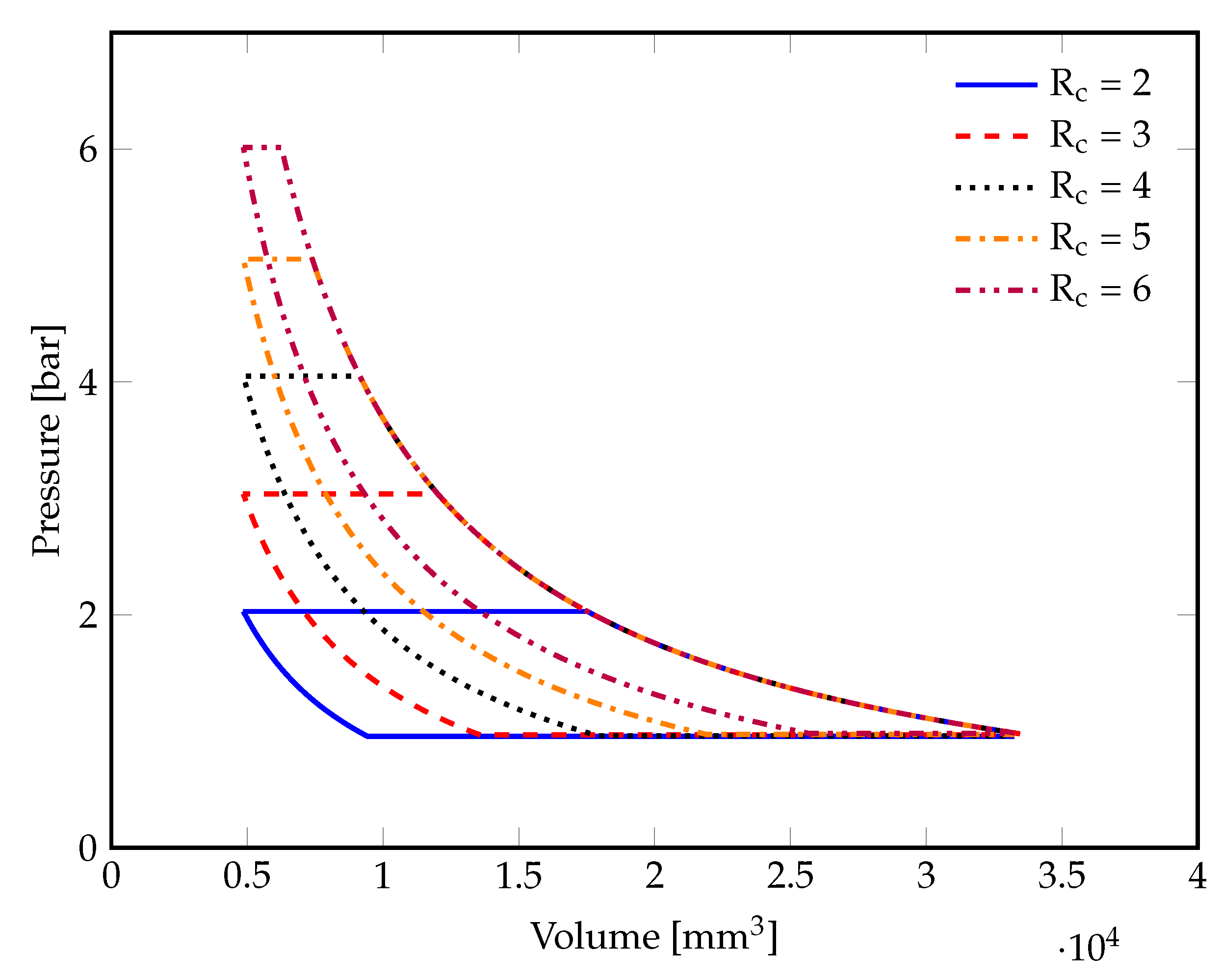
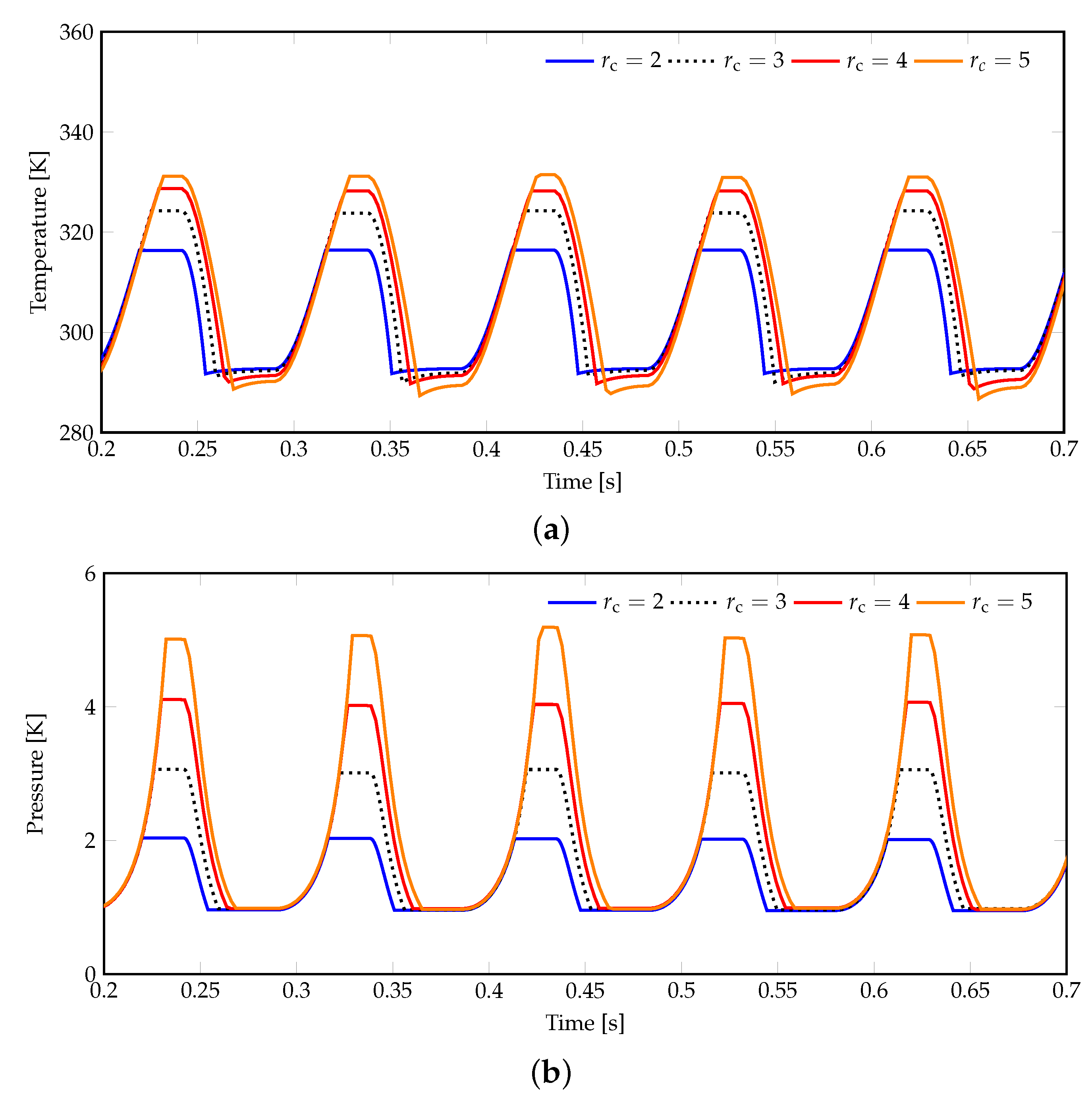
5.3. Pressure Ratio
6. Conclusions
Author Contributions
Funding
Data Availability Statement
Conflicts of Interest
References
- Lyu, L.; Chen, W.; Kan, A.; Zhang, Y.; Xue, S.; Zeng, J. Investigation of a Dual-Loop ORC for the Waste Heat Recovery of a Marine Main Engine. Energies 2022, 15, 8365. [Google Scholar] [CrossRef]
- Counsell, J.; Khalid, Y.; Stewart, M. Comparative performance modelling of heat pump based heating systems using dynamic carbon intensity. In Proceedings of the 11th IET International Conference on Advances in Power System Control, Operation and Management (APSCOM 2018), Hong Kong, China, 11–15 November 2018. [Google Scholar]
- Meibodi, S.S.; Loveridge, F. The future role of energy geostructures in fifth generation district heating and cooling networks. Energy 2022, 240, 122481. [Google Scholar] [CrossRef]
- Ocvirk, M.; Ristić, A.; Zabukovec Logar, N. Synthesis of Mesoporous γ-Alumina Support for Water Composite Sorbents for Low Temperature Sorption Heat Storage. Energies 2021, 14, 7809. [Google Scholar] [CrossRef]
- Bao, H.; Ma, Z.; Roskilly, A.P. A chemisorption power generation cycle with multi-stage expansion driven by low grade heat. Energy Convers. Manag. 2017, 150, 956–965. [Google Scholar] [CrossRef]
- Von Platen, B.C.; Munters, C.G. Refrigerator. US Patent US1685764A, 1 October 1925. [Google Scholar]
- Najjaran, A.; Freeman, J.; Ramos, A.; Markides, C.N. Experimental investigation of an ammonia-water-hydrogen diffusion absorption refrigerator. Appl. Energy 2019, 256, 113899. [Google Scholar] [CrossRef]
- Najjaran, A.; Harraz, A.A.; Mac Dowell, N.; Markides, C. Numerical and experimental investigation of diffusion absorption refrigeration systems for use with low-temperature heat sources. In Proceedings of the Ecos 2018—The 31st International Conference on Efficiency, Cost, Optimization, Simulation Furthermore, Environmental Impact Of Energy Systems, Guimaraes, Portugal, 17–22 June 2018; pp. 17–22. [Google Scholar]
- Rattner, A.S.; Garimella, S. Low-source-temperature diffusion absorption refrigeration. part II: Experiments and model assessment. Int. J. Refrig. 2016, 65, 312–329. [Google Scholar] [CrossRef] [Green Version]
- Rattner, A.S.; Garimella, S. Coupling-fluid heated bubble pump generators: Experiments and model development. Sci. Technol. Built Environ. 2015, 21, 332–347. [Google Scholar] [CrossRef]
- Ma, Z.; Bao, H.; Roskilly, A.P. Electricity-assisted thermochemical sorption system for seasonal solar energy storage. Energy Convers. Manag. 2020, 209, 112659. [Google Scholar] [CrossRef]
- Thinsurat, K.; Ma, Z.; Roskilly, A.P.; Bao, H. Compressor-assisted thermochemical sorption integrated with solar photovoltaic-thermal collector for seasonal solar thermal energy storage. Energy Convers. Manag. X 2022, 15, 100248. [Google Scholar] [CrossRef]
- Fitó, J.; Coronas, A.; Mauran, S.; Mazet, N.; Perier-Muzet, M.; Stitou, D. Hybrid system combining mechanical compression and thermochemical storage of ammonia vapor for cold production. Energy Convers. Manag. 2019, 180, 709–723. [Google Scholar] [CrossRef]
- Gao, P.; Hu, H.; Jin, S.; Wang, S.; Chen, Y.; Wu, W.; Yang, Q.; Zhu, F.; Wang, L. Solar-driven compression-assisted desorption chemisorption refrigeration/cold energy storage system. Energy Convers. Manag. 2022, 258, 115474. [Google Scholar] [CrossRef]
- Steger, D.; Feist, M.; Schlücker, E. Using a screw-type machine as reversible compressor–expander in a Carnot Battery: An analytical study towards efficiency. Appl. Energy 2022, 316, 118950. [Google Scholar] [CrossRef]
- Oh, S.; Wang, S.; Cho, S. Development of Energy Efficiency Design Map based on acoustic resonance frequency of suction muffler in compressor. Appl. Energy 2015, 150, 233–244. [Google Scholar] [CrossRef]
- Bianchi, G.; Cipollone, R. Theoretical modeling and experimental investigations for the improvement of the mechanical efficiency in sliding vane rotary compressors. Appl. Energy 2015, 142, 95–107. [Google Scholar] [CrossRef]
- Zhao, Y.; Xu, X.; Qadrdan, M.; Wu, J. Optimal operation of compressor units in gas networks to provide flexibility to power systems. Appl. Energy 2021, 290, 116740. [Google Scholar] [CrossRef]
- Meroni, A.; Zühlsdorf, B.; Elmegaard, B.; Haglind, F. Design of centrifugal compressors for heat pump systems. Appl. Energy 2018, 232, 139–156. [Google Scholar] [CrossRef]
- Uusitalo, A.; Turunen-Saaresti, T.; Honkatukia, J.; Tiainen, J.; Jaatinen-Värri, A. Numerical analysis of working fluids for large scale centrifugal compressor driven cascade heat pumps upgrading waste heat. Appl. Energy 2020, 269, 115056. [Google Scholar] [CrossRef]
- Tirnovan, R.; Giurgea, S.; Miraoui, A.; Cirrincione, M. Surrogate modelling of compressor characteristics for fuel-cell applications. Appl. Energy 2008, 85, 394–403. [Google Scholar] [CrossRef]
- Viholainen, J.; Grönman, K.; Jaatinen-Värri, A.; Grönman, A.; Ukkonen, P.; Luoranen, M. Centrifugal compressor efficiency improvement and its environmental impact in waste water treatment. Energy Convers. Manag. 2015, 101, 336–342. [Google Scholar] [CrossRef]
- Olsson, A.; Stemme, G.; Stemme, E. A numerical design study of the valveless diffuser pump using a lumped-mass model. J. Micromech. Microeng. 1999, 9, 34. [Google Scholar] [CrossRef]
- Venkatesan, J.; Nagarajan, G.; Seeniraj, R.; Murugan, R. Experimental validation of a mathematical model of a reed-valve reciprocating air compressor from an automotive-braking system. Int. J. Automot. Technol. 2010, 11, 317–322. [Google Scholar] [CrossRef]
- Sathe, A.A.; Groll, E.A.; Garimella, S.V. Analytical model for an electrostatically actuated miniature diaphragm compressor. J. Micromech. Microeng. 2008, 18, 035010. [Google Scholar] [CrossRef] [Green Version]
- Guan, D.; Cong, X.; Li, J.; Niu, Z. Experimental test and theoretical modeling on the working characteristics of spherical water pump. Flow Meas. Instrum. 2022, 85, 102162. [Google Scholar] [CrossRef]
- Adair, R.P.; Qvale, E.B.; Pearson, J.T. Instantaneous heat transfer to the cylinder wall in reciprocating compressors. In Proceedings of the International Compressor Engineering Conference, West Lafayette, IN, USA, 17–20 July 1972. [Google Scholar]
- Jia, X.; Zhao, Y.; Chen, J.; Peng, X. Research on the flowrate and diaphragm movement in a diaphragm compressor for a hydrogen refueling station. Int. J. Hydrog. Energy 2016, 41, 14842–14851. [Google Scholar] [CrossRef]
- Tuhovcak, J.; Hejčík, J.; Jícha, M. Modelling fluid flow in a reciprocating compressor. Epj. Web Conf. 2015, 92, 02100. [Google Scholar] [CrossRef] [Green Version]
- Picard, A.; Davis, R.; Gläser, M.; Fujii, K. Revised formula for the density of moist air (CIPM-2007). Metrologia 2008, 45, 149. [Google Scholar] [CrossRef]
- Lemmon, E.W.; Jacobsen, R.T.; Penoncello, S.G.; Friend, D.G. Thermodynamic properties of air and mixtures of nitrogen, argon, and oxygen from 60 to 2000 K at pressures to 2000 MPa. J. Phys. Chem. Ref. Data 2000, 29, 331–385. [Google Scholar] [CrossRef]


| Parameters | ||||||||
|---|---|---|---|---|---|---|---|---|
| Unit | [mm] | [mm] | [mm] | [mm] | [mm] | [mm] | [mm] | [mm] |
| Value | 116 | 10.17 | 95 | 90 | 3.47 | 49.5 | 3.35 | 97.16 |
| Process | Reynolds Number | a | b | c |
|---|---|---|---|---|
| Compression | 0.08 | 0.8 | 0.6 | |
| Discharge | 0.08 | 0.8 | 0.6 | |
| Expansion | 0.12 | 0.8 | 0.6 | |
| Suction | 0.08 | 0.9 | 0.6 |
| Pressure [bar] | 0 | 0.5 | 1 | 1.5 | 2 | 2.5 | 3 | 3.5 | 4 | 4.5 | 5 | 5.5 | 6 |
|---|---|---|---|---|---|---|---|---|---|---|---|---|---|
| Flow rate [Lit/min] | 42 | 38 | 35 | 32.5 | 30 | 29 | 26 | 25 | 22.5 | 20 | 19 | 16 | 14 |
| Temperature [°C] | 32.5 | 32.9 | 33 | 33.1 | 33.4 | 33.6 | 33.7 | 33.8 | 33.7 | 32.6 | 32.4 | 32.2 | 32.2 |
Disclaimer/Publisher’s Note: The statements, opinions and data contained in all publications are solely those of the individual author(s) and contributor(s) and not of MDPI and/or the editor(s). MDPI and/or the editor(s) disclaim responsibility for any injury to people or property resulting from any ideas, methods, instructions or products referred to in the content. |
© 2023 by the authors. Licensee MDPI, Basel, Switzerland. This article is an open access article distributed under the terms and conditions of the Creative Commons Attribution (CC BY) license (https://creativecommons.org/licenses/by/4.0/).
Share and Cite
Najjaran, A.; Meibodi, S.; Ma, Z.; Bao, H.; Roskilly, T. Experimentally Validated Modelling of an Oscillating Diaphragm Compressor for Chemisorption Energy Technology Applications. Energies 2023, 16, 489. https://doi.org/10.3390/en16010489
Najjaran A, Meibodi S, Ma Z, Bao H, Roskilly T. Experimentally Validated Modelling of an Oscillating Diaphragm Compressor for Chemisorption Energy Technology Applications. Energies. 2023; 16(1):489. https://doi.org/10.3390/en16010489
Chicago/Turabian StyleNajjaran, Ahmad, Saleh Meibodi, Zhiwei Ma, Huashan Bao, and Tony Roskilly. 2023. "Experimentally Validated Modelling of an Oscillating Diaphragm Compressor for Chemisorption Energy Technology Applications" Energies 16, no. 1: 489. https://doi.org/10.3390/en16010489