Fault Diagnosis of Wind Turbine Bearings Based on CEEMDAN-GWO-KELM

Abstract

To solve the problem of fault signals of wind turbine bearings being weak, not easy to extract, and difficult to identify, this paper proposes a fault diagnosis method for fan bearings based on Complete Ensemble Empirical Mode Decomposition with Adaptive Noise (CEEMDAN) and Grey Wolf Algorithm Optimization Kernel Extreme Learning Machine (GWO-KELM). First, eliminating the interference of noise on the collected vibration signal should be conducted, in which the wavelet threshold denoising approach is used in order to reduce the noise interference with the vibration signal. Next, CEEMDAN is used to decompose the signal after a denoising operation to obtain the multi-group intrinsic mode function (IMF), and the feature vector is selected by combining the correlation coefficients to eliminate the spurious feature components. Finally, the fuzzy entropy for the chosen IMF component is input into the GWO-KELM model as a feature vector for defect detection. After diagnosing the Case Western Reserve University (CWRU) dataset by the method presented in this research, it is found that the method can identify 99.42% of the various bearing states. When compared to existing combination approaches, the proposed method is shown to be more efficient for diagnosing wind turbine bearing faults.

1. Introduction

As a kind of renewable and clean energy source, research on wind energy has developed rapidly in recent years [1]. Wind turbines are a key piece of equipment in wind power generation systems due to their long-term operation in the field in relatively harsh environments, resulting in their frequent failure. As an important part of the fan drive system, the operating condition of the rolling bearings often directly affects the performance of the whole machine [2]. Therefore, it is crucial to monitor and diagnose the rolling bearings of wind turbines in order to improve the safe and stable operation of machinery, lower maintenance costs, and increase the financial advantages of operating a wind farm.

In practical engineering, the fault vibration signal collected by people is nonlinear and non-stationary, and there is noise to a large extent. The method of wavelet threshold denoising [3] can be effective for the noise reduction of vibration signals. Regarding the extraction of fault features, the conventional wind turbine vibration signal processing approach is unable to reliably produce an accurate judgment of wind turbine fault [4]. Empirical Mode Decomposition (EMD) was first proposed by Huang et al. [5], which reduces the algorithm decomposition error caused by human factors and is widely applied to fault diagnosis [6], signal denoising [7], medicine [8], and other fields. Due to the defects of EMD theory, the decomposed signals will result in the modal aliasing phenomenon and end-point effects. To resolve this problem, Wu et al. developed Ensemble Empirical Mode Decomposition (EEMD) [9], an enhanced algorithm of EMD. It adds white Gaussian noise to the original signal to eliminate the mode aliasing phenomenon in the process of EMD decomposition as far as possible; however, there is a lot of noise residual in its reconstructed signal. Torres et al. proposed a new improved algorithm named complete ensemble empirical mode decomposition with adaptive noise (CEEMDAN) [10]. This algorithm can well process nonlinear and non-stationary signals, effectively reducing the reconstruction error of EEMD with high decomposition efficiency and good decomposition effect. Colominas et al. [11] have improved CEEMDAN and successfully tested it on several biomedical signals. Wang and Shao [12] used reweighted CEEMDAN denoising to extract fault features. Hassan et al. [13] used CEEMDAN decomposition to identify seizures.

One of the crucial processes in mechanical problem diagnostics is feature extraction. In recent years, dimensionless parameters have been added to the feature extraction of mechanical equipment vibration signals, including approximate entropy, sample entropy, and fuzzy entropy. Sampaio et al. [14] used the approximate entropy algorithm to the vibration signal of the crack axis to detect the crack and its depth. Wang et al. [15] accurately classified the fault samples of rolling bearings using the generalized fine composite multi-scale sample entropy algorithm. Effective feature selection for diagnosing chattering vibrations was achieved by Tran et al. [16] using fuzzy entropy and a similarity classifier. After feature extraction, a suitable classification algorithm is needed to implement fault diagnosis. The single-layer feed-forward neural network Extreme Learning Machine (ELM) [17] has good learning ability and generalization ability, so its application field is very wide. Yang et al. [18] used the ELM algorithm to predict the degree of roasting of cocoa beans. Li et al. [19] established a model based on MPA-ELM to predict the thermal displacement of the electric spindle. Katılmış et al. [20] used an ELM classifier in a sign language recognition system. Diker et al. [21] improved the classification performance of ECG signals using the DEA-ELM method. He et al. [22] used the reverse cognition drosophila optimization algorithm to optimize ELM parameters and established a rolling bearing fault diagnosis model. However, ELM makes the classification results fluctuate and the stability is relatively poor. For this reason, Huang et al. [23] introduced kernel mapping in ELM instead of random mapping, which enhanced its stability and generalization ability. Hu et al. [24] used the particle swarm algorithm to optimize KELM for planetary gearbox problem detection in wind turbines and achieved certain results.

To sum up, this research suggests a method for detecting wind turbine bearing problems based on CEEMDAN-GWO-KELM, aiming at the issue that it is challenging to accurately extract various operating states of wind turbine bearings in an environment with a lot of background noise. Firstly, use the wavelet threshold denoising method to denoise the bearing defect signal, then the denoised signal is subjected to CEEMDAN decomposition to produce a series of IMF components. The first four IMFs with rich bearing characteristic information are selected by the correlation coefficient, and the fuzzy entropy of the first four IMFs is calculated. Finally, to diagnose wind turbine bearing faults by inputting the fuzzy entropy as a feature vector into the GWO-KELM model. This method has proven efficient for diagnosing wind turbine bearing faults when compared with other combination methods.

2. Fundamental

2.1. Wavelet Threshold Denoising

Wavelet threshold denoising is the decomposition of the signal containing noise at each scale by wavelet, and all the decomposition values at a large scale (low resolution) are retained. Both the soft threshold method and the hard threshold method can be applied to cope with small-scale (high-resolution) decomposition values. Finally, the wavelet transform is used for reconstruction, and the effective signal is recovered. The basic principle is shown in Figure 1. Wavelet threshold denoising functions usually include both soft thresholding and hard thresholding. The methods of soft threshold and hard threshold denoising differ. The generated signal is as smooth as the original signal because of the excellent continuity of the soft threshold denoising method; however, the hard threshold denoising method lacks smoothness. Therefore, the soft threshold denoising method is used in this research. For soft threshold expression, see Formula (1):

$$\omega \lambda =\left\{\begin{array}{ll}\left[sign(\omega )\right](\left|\omega \right|-\lambda ),& \left|\omega \right|\ge \lambda \\ 0,& \left|\omega \right|<\lambda \end{array}\right.$$

(1)

Among them, $sign\left(·\right)$ is a symbolic function; $\omega$ is the magnitude of the wavelet coefficients; $\omega \lambda$ is the magnitude of wavelet coefficients after adding the threshold; and $\lambda$ is the threshold.

In this study, the threshold value needs to be obtained by using the $wden$ function in MATLAB. Here, $wden$ uses a function in the wavelet toolbox of MATLAB R2019a. The wavelet coefficients need to be obtained by the $wden$ function using the specified orthogonal or double orthogonal wavelets to perform N-level wavelet decomposition of the signal. For the $wden$ function, see Formula (2):

$$xd=wden\mathrm{(}x,tptr,sorh,scal,n,wname\mathrm{)}$$

(2)

In the formula, $xd$ is a denoised signal by wavelet thresholding; x is the original signal; $tptr$ is the threshold selection criterion; $sorh$ is the threshold selection method; n is the number of layers to be decomposed; and $wname$ is the wavelet basis function.

2.2. CEEMDAN Algorithm

Based on the foundation of EMD, CEEMDAN also takes the concept of averaging by multiple superpositions while incorporating white Gaussian noise into the original signal. Here are the steps to break it down:

Step 1: Construct the signal $X\left(t\right)$, as shown in Formula (3):

$$X(t)=x(t)+{\epsilon }_0{\omega }_i(t)$$

(3)

In the formula, $x\left(t\right)$ is the original signal; $X\left(t\right)$ is the signal after adding white noise; ${\epsilon }_0$ is the amplitude; and ${\omega }_i(t)(i=1,2,\dots ,N)$ is white noise.

Step 2: The signal X(t) was decomposed by EMD to obtain the first-order modal component, as shown in Formula (4):

$$IM{F}_1(n)=\frac{1}{N}{\displaystyle \sum _{i=1}^{N}IM{F}_1^i(n)}$$

(4)

Step 3: After the first-order modal component is obtained, the first residual component is calculated, as shown in Formula (5):

$$r_1(n)=x(n)-IM{F}_1(n)$$

(5)

Step 4: Through the obtained $r_1\left(n\right)$, decompose again to obtain the second-order modal component, as shown in Formula (6):

$$IM{F}_2(n)=\frac{1}{N}{\displaystyle \sum _{i=1}^N{E}_1\left\{r_1(n)+{\epsilon }_1{E}_1\left[{\omega }^i(n)\right]\right\}}$$

(6)

Step 5: Calculate the $j$th order residual component from $j=2,3,\cdots$ to obtain the $j+1$th order modal component, then the $j$th residual component and the modal component, as shown in Formulas (7) and (8):

$${\mathrm{r}}_j(n)=r_{j-1}(n)-IM{F}_n(n)$$

(7)

$$IM{F}_j(n)=\frac{1}{N}{\displaystyle \sum _{i=1}^N{E}_1\left\{r_j(n)+{\epsilon }_j{E}_j\left[{\omega }^i(n)\right]\right\}}$$

(8)

In the formula, $E_j\left(·\right)$ is the $j$th-order modal component.

Step 6: Repeat the above steps until there are no more than two extreme points of the residual signal. When the algorithm is terminated, the $j$-order modal component can be obtained, and the final residual signal is shown in Formula (9):

$$r(n)=x(n)-{\displaystyle \sum _{j=1}^{J}IM{F}_j}$$

(9)

Finally, the original signal after decomposition is shown in Formula (10):

$$x(n)={\displaystyle \sum _{j=1}^{J}IM{F}_j+r(n)}$$

(10)

2.3. Fuzzy Entropy

Fuzzy Entropy is improved on the basis of sample entropy and is a quantitative statistical indicator of signal complexity. It is different from sample entropy in that sample entropy uses a unit step function, which has a large mutation and lacks the continuity of an entropy value. The value of the threshold is sensitive to it, and its weak change may lead to the mutation of the sample entropy value. Fuzzy entropy combines fuzzy set theory and uses a fuzzy membership function as the hard threshold criterion in entropy. This paper constructs the feature vector based on the fuzzy entropy of the $IMF$ component after Pearson correlation coefficient selection to characterize the state information contained in the signal. The specific calculation process of fuzzy entropy is as follows:

Step 1: With respect to a time series of length $N$ $\left\{x(i),i=1,2,\dots ,N\right\}$, initialize the embedding dimension $m$. The above time series is reconstructed in phase space, as shown in Formula (11):

$$X(i)=\left\{x(i),x(i+1),\dots ,x(i+m-1)\right\}-u(i)$$

(11)

In the formula, $X\left(i\right)$ is the new time series after reconstruction, $i=1,2,\dots ,N-m+1$,$\mathrm{and} u\left(i\right)$ is the average value of $m$ consecutive $x\left(i\right)$, as shown in Formula (12):

$$u_i=\frac{1}{m}{\displaystyle \sum _{k=0}^{m-1}x(i+k)}$$

(12)

Step 2: Definition of the distance between two vectors $X\left(i\right)$ and $X\left(j\right)$ for the difference in the corresponding element of absolute value maximum, as shown in Formula (13):

$$d_{ij}^m=\max \left\{\left|(x(i+k)-u(i))-(x(j+k)-u(i))\right|\right\}$$

(13)

In the formula, $1\le i,j\le N-m+1$, and $i\ne j$.

Step 3: To define the similarity, introduce a fuzzy membership function between vectors $X\left(i\right)$ and $X\left(j\right)$, as shown in Formula (14):

$$A_{ij}^m\left\{\begin{array}{cc}1,& d_{ij}^m=0\\ \exp \left[-\ln (2){(\frac{d_{ij}^m}{r})}^2\right],& d_{ij}^m>0\end{array}\right.$$

(14)

In the formula, $r$ is the similarity tolerance parameter, $\delta$ is the standard deviation of the original 1D time series, define the relationship between the two as: $r=R\times \delta$.

Step 4: Define the function $C_i^m\left(r\right)$, as shown in Formula (15):

$$C_i^m(r)=\frac{1}{N-m}{\displaystyle \sum _{j=1,j\ne i}^{N-m+1}{A}_{ij}^m}$$

(15)

Then, the relation dimension under $m$ dimension can be obtained, as shown in Formula (16):

$${\Phi }^m(r)=\frac{1}{N-m}{\displaystyle \sum _{i=1}^{N-m+1}{C}_i^m(r)}$$

(16)

Step 5: Increase the embedding dimension by 1, and then repeat the above steps 1 to 4 for the $m+1$ dimension vector to obtain the relational dimension ${\Phi }^{m+1}\left(r\right)$ in the $m+1$ dimension, as shown in Formula (17):

$${\Phi }^{m+1}(r)=\frac{1}{N-m}{\displaystyle \sum _{i=1}^{N-m}{C}_i^{m+1}(r)}$$

(17)

Step 6: Finally, the expression of fuzzy entropy can be obtained as:

$$FuzzyEn(m,r,N)=\ln {\Phi }^m(r)-\ln {\Phi }^{m+1}(r)$$

(18)

In the formula, $m$ is the embedding dimension parameter, and $N$ is the original time series length.

3. Fault Diagnosis Based on GWO-KELM

3.1. Grey Wolf Optimization Algorithm

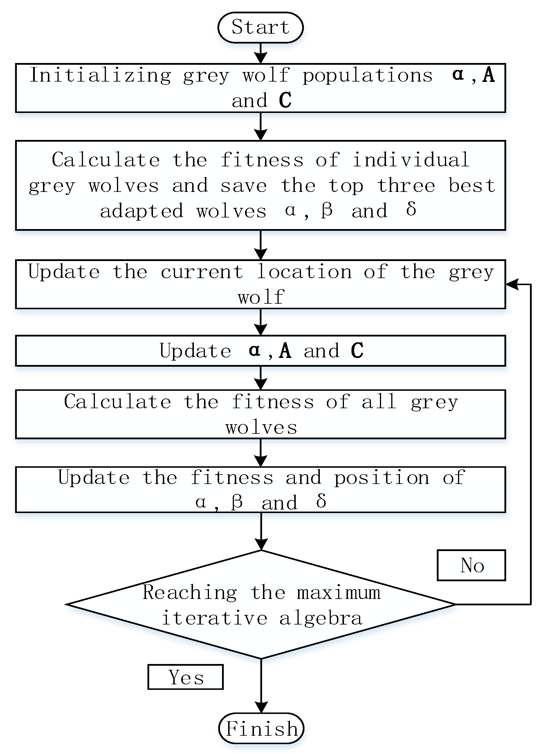
The grey wolf optimization algorithm is a new intelligent optimization algorithm for simulating the social hierarchy and hunting behavior of wolf packs. This algorithm has strong convergence and fewer parameters. The flow chart of the GWO algorithm is shown in Figure 2. There are four social classes of wolves in GWO, in which the $\alpha$ wolves have the highest rank and lead the other wolves; the second is the $\beta$ wolves, which help the $\alpha$ wolves make decisions; and the $\delta$ wolves follow the first two wolves and command the $\omega$ wolves; finally, the $\omega$ wolves, who are subordinate to the $\alpha$, $\beta$, and $\delta$ wolves. The first three types of wolves hunt down their prey, and the last wolves track and encircle them to achieve the purpose of catching their prey [25]. The process of the GWO algorithm is as follows:

Step 1: Surround the prey. In pursuit of their prey, the wolves surround it first. The mathematical modeling of this behavior is:

$$\left\{\begin{array}{l}\mathit{D}=\left|\mathit{C}\cdot {\mathit{X}}_P\left(t\right)-\mathit{X}\left(t\right)\right|\\ \mathit{X}\left(t+1\right)={\mathit{X}}_P\left(t\right)-\mathit{A}\cdot D\end{array}\right.$$

(19)

$$\left\{\begin{array}{l}\mathit{A}=2\mathit{A}{\mathit{r}}_1-\mathit{A}\\ \mathit{C}=2{\mathit{r}}_2\end{array}\right.$$

(20)

In the formula, $\mathit{D}$ is the distance between grey wolf and prey; ${\mathit{X}}_P\left(t\right)$ is the current position of the prey; $t$ is the number of iterations; $\mathit{X}\left(t\right)$ is the current position of the grey wolf; ${\mathit{r}}_1,{\mathit{r}}_2\in \left[0,1\right]$; $\alpha$ is the convergence factor; and $\mathit{A}$ and $\mathit{C}$ are the coefficient vectors.

Step 2: Hunt down the prey. When the grey wolf identifies the location of the prey, $\alpha$ leads $\beta$ and $\delta$ to guide the wolf pack to surround the prey. Mathematically modeled as:

$$\left\{\begin{array}{l}{\mathit{D}}_{\alpha }=\left|{\mathit{C}}_1\cdot {\mathit{X}}_{\alpha }-\mathit{X}\right|\\ {\mathit{D}}_{\beta }=\left|{\mathit{C}}_2\cdot {\mathit{X}}_{\beta }-\mathit{X}\right|\\ {\mathit{D}}_{\delta }=\left|{\mathit{C}}_3\cdot {\mathit{X}}_{\delta }-\mathit{X}\right|\end{array}\right.$$

(21)

In the formula, $\mathit{X}$ is the current wolf position; ${\mathit{C}}_1$, ${\mathit{C}}_2$, and ${\mathit{C}}_3$ correspond to coefficient vectors of $\alpha$, $\beta ,$ and $\delta$; ${\mathit{D}}_{\alpha }$, ${\mathit{D}}_{\beta }$, and ${\mathit{D}}_{\delta }$ represent the distances between $\alpha$, $\beta$, and $\delta$ and the prey, respectively; and ${\mathit{X}}_{\alpha }$, ${\mathit{X}}_{\beta }$, and ${\mathit{X}}_{\delta }$ represent the location of the corresponding wolf pack at the moment.

Step 3: Update individual grey wolf.

$$\left\{\begin{array}{l}{\mathit{X}}_1={\mathit{X}}_{\alpha }-{\mathit{A}}_1\cdot {\mathit{D}}_{\alpha }\\ {\mathit{X}}_2={\mathit{X}}_{\beta }-{\mathit{A}}_2\cdot {\mathit{D}}_{\beta }\\ {\mathit{X}}_3={\mathit{X}}_{\delta }-{\mathit{A}}_3\cdot {\mathit{D}}_{\delta }\end{array}\right.$$

(22)

$$\mathit{X}\left(t+1\right)=\frac{{\mathit{X}}_1+{\mathit{X}}_2+{\mathit{X}}_3}{3}$$

(23)

In the formula, ${\mathit{A}}_1$, ${\mathit{A}}_2$, and ${\mathit{A}}_3$ correspond to coefficient vectors of α, β, and δ; ${\mathit{X}}_1$, ${\mathit{X}}_2$, and ${\mathit{X}}_3$ represent the direction vectors that $\alpha$, $\beta$, and $\delta$ guide $\omega$ to move in the next step; and $\mathit{X}\left(t+1\right)$ represents the place of the candidate wolf that the three wolf packs produced.

3.2. Kernel Extreme Learning Machine (KELM)

Huang and others proposed ELM for the first time in 2006. It performs generalization well and learns incredibly and quickly. The difference between KELM and the ELM algorithm is that a kernel function is added on the basis of achieving the purpose of enhancing the stability and generalization of the ELM algorithm. The traditional ELM algorithm expression is:

$$\phi \left(x\right)=h\left(x\right)\beta$$

(24)

$$H=h\left(x\right)={\left[\begin{array}{cc}g\left({\omega }_1{x}_1+b_1\right)\hspace{1em}\cdots & g\left({\omega }_k{x}_1+b_k\right)\\ ⋮& ⋮\\ g\left({\omega }_1{x}_N+b_1\right)\hspace{1em}\cdots & g\left({\omega }_k{x}_N+b_k\right)\end{array}\right]}_{N\times k}$$

(25)

$$\beta =H^{+}T$$

(26)

$$H^{+}=H^T{\left(H{H}^T\right)}^{-1}$$

(27)

In the formula, $N$ is the number of samples; $\omega$ is the weight between input and output; $b$ is the bias of the hidden layer; $H$ is the output matrix of the hidden layer; $H^{+}$ is the generalized inverse matrix of $H$; $\beta$ is the vector of weights between the output and the hidden layer; $g()$ is activation function; $k$ is the quantity of concealed units; $\mathrm{and} T$ is the target matrix for the training set.

KELM makes the kernel mapping in the model more stable by introducing kernel functions. The expression of the KELM algorithm is:

$$\phi \left(x\right)=h\left(x\right)H^T{\left(\frac{I}{C}+H{H}^T\right)}^{-1}T=\left[\begin{array}{l}\mathrm{k}\left(x,x_1\right)\\ ⋮\\ \mathrm{k}\left(x,x_N\right)\end{array}\right]{\left(\frac{I}{C}+H{H}^T\right)}^{-1}T$$

(28)

In the formula, $C$ is the regularization parameter; $I$ is an $N$ order unit matrix; and $k\left(A,b\right)$ is the kernel function; here, the RBF kernel function is adopted and is needed to set the kernel parameter $\gamma$.

3.3. GWO Optimizes the KELM Model

In this study, the Kernel Extreme Learning Machine is optimized using the grey wolf method. In the GWO-KELM model, GWO is used to optimize the parameters $C$ and $\gamma$ of KELM. The radial basis function is chosen as the KELM kernel function in this study. Figure 3 depicts the GWO-KELM process, and the specific operational process is described as follows:

Step 1: Input data.

Step 2: GWO and KELM parameters are initialized, including population size, iteration times, regularization coefficient, and kernel parameters, and KELM recognition accuracy is taken as the fitness function.

Step 3: Randomly generate Wolf pack positions within the set range.

Step 4: Determine the value of the wolf pack’s fitness function at its current location.

Step 5: Wolves are divided into $\alpha$, $\beta ,$ and $\delta$ groups according to their fitness.

Step 6: Update the wolf pack location and fitness function values.

Step 7: Check to see if the desired number of iterations is reached, if not, return to step 5; otherwise, the optimization ends, and the output is the optimal parameters $C$ and $\gamma$.

Step 8: Train KELM with optimal parameters for fault classification.

3.4. Fault Diagnosis Model

Based on CEEMDAN-GWO-KELM wind turbine bearing fault diagnosis method is depicted in Figure 4 and involves the following steps:

Step 1: The acquisition of vibration signals, the acceleration signal data of various bearing states are gathered at a specific sample frequency.

Step 2: In data preprocessing, first use the wavelet threshold denoising method for noise reduction processing, then decompose the denoised signal by the method of CEEMDAN and obtain some $IMF$ components.

Step 3: Feature extraction, calculate fuzzy entropy of each $IMF$ component. The fuzzy entropy of the first four-order IMF components is selected by the correlation coefficient, and constructs the feature vector.

Step 4: Normalization processing, normalizing the extracted fault feature dataset.

Step 5: In fault diagnosis, use the processed feature dataset as the GWO-KELM fault classifier’s input to achieve fault diagnosis.

4. Experimental Data Processing and Analysis

4.1. Data Collection and Preprocessing

This article used Case Western Reserve University (CWRU) bearing simulation experiment data centers to evaluate the accuracy and efficacy of CEEMDAN-GWO-KELM methods in wind turbine bearing defect diagnostics. A driver, a torque sensor, a load click, and a test bearing make up the test bench, as shown in Figure 5.

In the bearing experiment of CWRU, the motor shaft is supported by the bearing that will be tested. The drive end bearing model number SKF6205 has sampling rates of 12 and 48 kHz, respectively; SKF6203 is the fan end bearing, while 12 KHz is the sampling frequency. Its working principle is similar to that of the wind turbine drive chain, and the rotational speeds of the bearings in the CWRU dataset are 1730 rpm, 1750 rpm, 1772 rpm, and 1797 rpm, which are within the rotational speed range of the wind turbine bearings. The driving characteristics and the CWRU bearing test bench’s rotating speed are similar to those of the wind turbine bearing; consequently, this dataset is used to verify the algorithm proposed in this research.

In order to confirm the algorithm’s efficacy in fault diagnosis, the normal operating data and damage diameters of the bearing at a rotational speed of 1730 rpm and a sampling frequency of 12 KHz are selected as 0.1778 mm (0.007 inches), 0.3556 (0.014 inches), and 0.5334 (0.021 inches) operating data for inner ring failure, outer ring failure, and rolling element failure. The normal bearings are grouped into one group and the remaining faulty bearings are grouped into nine groups. As a result, ten labels in total are defined, as seen in

Table 1. Fault type and fault code.

Fault Type	Fault Size (mm)	Fault Code
Inner ring fault 1	0.1778	1
Inner ring fault 2	0.3556	2
Inner ring fault 3	0.5334	3
Outer ring fault 1	0.1778	4
Outer ring fault 2	0.3556	5
Outer ring fault 3	0.5334	6
Rolling element failure 1	0.1778	7
Rolling element failure 2	0.3556	8
Rolling element failure 3	0.5334	9
normal	0	10

. The original data sample length is divided into 2048 points, each state signal has 30 groups, and the length of each group of signals is 2048.

In order to understand the process more intuitively, the bearing example of the inner ring fault is used to discuss. Figure 6 displays the experimental signal and the inner ring fault’s frequency spectrum. Although the signal clearly exhibits shock characteristics, it cannot directly determine the type of fault, so a further process is needed.

4.2. Feature Extraction Based on CEEMDAN Decomposition

The inner ring fault signal after noise removal is broken down by CEEMDAN, and decomposition yields a number of $IMF$ components. The larger the order, the lower the frequency; that is, the less fault information it contains.

In order to accurately extract the $IMF$ components with more fault signals, the correlation coefficient is selected to screen each modal component. The correlation coefficient of each $IMF$ is calculated. In order to further screen out the appropriate components, the correlation coefficient of the $IMFs$ of ten different fault signals is calculated. The first seven $IMF$ correlation coefficients of the ten fault types are shown in

Table 2. $IMF$ correlation coefficient of ten fault types.

Fault Type	$$\mathit{I}\mathit{M}{\mathit{F}}_1$$	$$\mathit{I}\mathit{M}{\mathit{F}}_2$$	$$\mathit{I}\mathit{M}{\mathit{F}}_3$$	$$\mathit{I}\mathit{M}{\mathit{F}}_4$$	$$\mathit{I}\mathit{M}{\mathit{F}}_5$$	$$\mathit{I}\mathit{M}{\mathit{F}}_6$$	$$\mathit{I}\mathit{M}{\mathit{F}}_7$$	Fault Code
Inner ring fault 1	0.914429	0.382676	0.254300	0.144165	0.102502	0.047260	0.029596	1
Inner ring fault 2	0.907739	0.428273	0.318125	0.125363	0.108809	0.074792	0.044658	2
Inner ring fault 3	0.987412	0.141102	0.100381	0.079551	0.082432	0.051613	0.023653	3
Outer ring fault 1	0.978397	0.260789	0.039529	0.006446	0.017525	0.017619	0.007012	4
Outer ring fault 2	0.398757	0.159746	0.336387	0.521029	0.560815	0.627021	0.413391	5
Outer ring fault 3	0.965937	0.150558	0.145045	0.168494	0.068543	0.021311	0.013905	6
Rolling element failure 1	0.348466	0.224356	0.160948	0.379321	0.619729	0.72292	0.303485	7
Rolling element failure 2	0.752964	0.379008	0.422717	0.400106	0.468957	0.166869	0.085792	8
Rolling element failure 3	0.714964	0.463578	0.528637	0.379162	0.357800	0.339578	0.151980	9
normal	0.468767	0.530276	0.596383	0.515570	0.430901	0.506312	0.439301	10

.

The table above demonstrates that the correlation coefficients between the $IMF$ components of the first four faults and the original signals are large, most of which are more than 0.1, while the correlation coefficients of the latter are mostly lower than 0.1, or even tend to 0. From this, it can be concluded that the first four $IMF$ components have the largest correlation with the original signal and contain the primary fault information. Therefore, the fuzzy entropy of the first four $IMF$ components is determined as the feature vector, and the remainder is employed as a false component to be eliminated.

Fuzzy entropy can characterize fault characteristics to a certain extent, and the fuzzy entropy characteristic values under 10 states are as displayed in

Table 3. IMF Component Fuzzy Entropy of CEEMDAN Decomposition.

Fault Type	$\mathit{I}\mathit{M}{\mathit{F}}_1$	$\mathit{I}\mathit{M}{\mathit{F}}_2$	$\mathit{I}\mathit{M}{\mathit{F}}_3$	$\mathit{I}\mathit{M}{\mathit{F}}_4$	Fault Code
Inner ring fault 1	0.434972	0.177999	0.113561	0.031011	1
Inner ring fault 2	0.195311	0.096538	0.113142	0.017670	2
Inner ring fault 3	0.448848	0.114559	0.07165	0.022327	3
Outer ring fault 1	0.276833	0.172664	0.099691	0.02737	4
Outer ring fault 2	0.043899	0.028376	0.008482	0.009212	5
Outer ring fault 3	0.234330	0.093997	0.089899	0.062964	6
Rolling element failure 1	0.028447	0.006922	0.007336	0.002261	7
Rolling element failure 2	0.265729	0.05313	0.076417	0.015427	8
Rolling element failure 3	0.115616	0.039859	0.038023	0.009757	9
normal	0.198319	0.018702	0.068489	0.037776	10

.

4.3. Experimental Comparative Analysis

In order to confirm the superiority and precision of the GWO-KELM diagnostic model proposed in this paper, the GWO-KELM model is compared with the other three models including the KELM model, GOA-KELM model, and WOA-KELM, to verify the efficiency of each method’s classification.

The fuzzy entropy values of the first four IMF components of each fault type constitute a 300 × 4 fault feature matrix and input it into the GWO-KELM model. Eighteen groups of feature vectors in each state were picked at random to serve as training samples, and the remaining 12 groups of feature vectors were selected as test samples. The number of wolves in the GWO-KELM model was set as 20, and 30 iterations was the set maximum number of iterations. Figure 7a presents the diagnostic findings. To demonstrate the classification impact of the model, the WOA-KELM, GOA-KELM, and KELM models were tested with this test set, and Figure 7b–d displays the diagnostic outcomes.

Figure 7 shows that the GWO-KELM model suggested in this paper has a classification accuracy of 99.17%, while the classification accuracy of the WOA-KELM, GOA-KELM, and KELM models is 98.33%, 96.67%, and 93.33%, respectively. A single test cannot accurately depict the model’s classification accuracy. For the validity and veracity of the experimental findings, the experiments were repeated 20 times on the four models, respectively, and the average value of classification accuracy was used as the foundation. The obtained diagnostic results obtained are depicted in

Table 4. Comparison of results of different models.

Diagnostic Model	Average Training Accuracy	Average Test Accuracy
KELM	93.75%	92.29%
GOA-KELM	98.28%	97.06%
WOA-KELM	100%	98.73%
GWO-KELM	100%	99.42%

.

As seen in Table 4, the average training accuracy of the GWO-KELM model used in this paper is 100%, and the average test accuracy is 99.42%, which is better than the KELM, GOA-KELM, and WOA-KELM models. Therefore, the method proposed in this paper is superior to other diagnostic methods and has certain superiority in rolling bearing fault diagnosis.

5. Conclusions

In summary, aiming at the issue of rolling bearing malfunction identification and diagnosis, the bearing defect diagnosis approach proposed in this paper combines wavelet threshold denoising, CEEMDAN fuzzy entropy, and GWO-KELM. Based on a comparative experiment, this method’s efficacy and accuracy are confirmed, which has certain advantages in wind turbine fault diagnosis.

The wavelet threshold denoising approach is used to pretreat the bearing vibration signal, which can reduce noise interference with the vibration signal.

The application of CEEMDAN decomposition to fan-bearing fault diagnosis has greatly reduced the mode aliasing problem. The fuzzy entropy of effective components selected by the Pearson correlation coefficient can better reflect the fault characteristic information of bearings.

By diagnosing various bearing states using the measured bearing data from the CWRU bearing test bench, the validity of the method provided in this work is demonstrated. The experimental comparison shows that the method has higher diagnostic accuracy.