Article

Design and Implementation of a Driving Strategy for Star-Connected Active Magnetic Bearings with Application to Sensorless Driving

Laboratory of Actuation Technology, Saarland University, 66123 Saarbrücken, Germany
*
Author to whom correspondence should be addressed.
Energies 2023, 16(1), 396; https://doi.org/10.3390/en16010396
Submission received: 18 November 2022 / Revised: 12 December 2022 / Accepted: 21 December 2022 / Published: 29 December 2022
(This article belongs to the Section F3: Power Electronics)

Abstract

:
For decades, sensorless position estimation methods gained lots of interest from the research community, especially in the field of electric drives and active magnetic bearings (AMBs). In particular, the direct flux control (DFC) technique promises unique advantages over other sensorless techniques, such as a higher bandwidth, but on the other hand, it requires the coils to be connected in a star topology. Until now, star-point connections are rarely found on active magnetic bearings. In consequence, there is no known publication about the application of the DFC to an AMB to this date. In order to apply the DFC to an AMB, a star-point driving approach for AMBs must be developed beforehand. A star-connected driving approach, capable of driving a four-phase AMB, is proposed and validated against traditional H-bridges in a simulation. Further, the strategy is tested in a physical application and generalised for 4 n phases. In terms of current dynamics, the simulation results can be compared to the well-known full H-bridge driving. The experiments on the physical application show that the actual current in the coils follows a reference with satisfactory accuracy. Moreover, the inductance measurements of the coils show a strong dependency on the rotor’s position, which is crucial for sensorless operation. A star-point connection delivers a satisfying response behaviour in an AMB application, which makes sensorless techniques that require a star point, such as the DFC, applicable to active magnetic bearings.

1. Introduction

Compared to classical mechanical bearings, active magnetic bearings (AMBs) offer unique properties due to a lack of mechanical contact and have, therefore, attracted tremendous interest in research and industry. In particular, they drastically reduce the mechanical friction at the rotor with the advantage of reduced wear, acoustic noise, maintenance cost and lubrication, as well as increased efficiency and a higher rotational speed when applied to electrical machines [1]. Thus, the economic and ecological impact of those machines can be improved significantly. The here-considered AMBs are based on magnetic reluctance forces, and consequently, they are inherently unstable systems. Hence, AMBs require control algorithms with position feedback in order to stabilise the rotor at the centre position [1]. The position feedback is realised conventionally by additional sensors, such as laser- or hall-effect sensors. Nevertheless, the sensors increase the cost, size and maintenance effort of the overall system, therefore weakening the economic merits of AMBs. In the past decades, sensorless control has been widely applied to AMBs to retrieve position information from electrical quantities already being measured in the system. Such a self-sensing approach can replace position sensors in cost-critical applications or provide further redundancy with existing position sensors in use cases where high functional safety is required.
Self-sensing for AMBs started decades ago with the application of observers [1], such as Luenberger observers, based on a linearised model [2]. The following works are based on signal modulation and therefore inject a time-varying signal into the AMB and evaluate the current response dependent on the air gap [3]. Such an approach offers an increased disturbance rejection. Another approach is based on processing the current ripple induced by a switching power amplifier. Such amplifiers are usually driven by a pulse-width-modulated (PWM) voltage that inherently injects a high-frequency signal into the AMB. The slope of the resulting current ripple depends on the inductance and, consequently, on the actual position and can be processed for position estimation [1,4,5]. Common limitations are bandwidth restrictions as well as a saturation of the inductance at higher currents that allows no robust position estimation in these working points. Another interesting attempt for self-sensing is based on the exploitation of the star-point voltage of a three-phase AMB. In particular [6], a high-frequency component is injected into an AMB, and the resulting voltage response at the neutral point of the AMB is measured. The work verified the effectiveness of the approach. Nevertheless, a poor signal-to-noise ratio (SNR) was obtained because the voltage at the star point is too small to be measured accurately. Especially for small low-power AMBs, the evaluation of the star-point voltage seems desirable because the current sensor measurements can be avoided for self-sensing, which is usually characterised by a small bandwidth and a small SNR for machines in the low- power region.
In the field of electrical machines, other sensorless algorithms were developed over the decades, based on either the induced back-EMF or machine anisotropies. The review works [7,8,9] provide a good overview of the existing techniques. In particular, there also exists a technique under the name of direct flux control (DFC), which successfully exploits the star-point voltage [10,11,12,13,14,15]. These works demonstrate the robustness, accuracy and increased SNR of this approach. More in detail, there is another circuitry based on a re-settable integrator circuit that allows to amplify the star-point voltage with an increased SNR.
This approach seems interesting for future research works. Nevertheless, the DFC technique requires not only an accessible star point but also the modification of the PWM pattern. In particular, this modification is performed using zero voltage vectors and dedicated voltage vectors for measurement. This puts several requirements on the switching power amplifier that is used. Because AMBs usually only need one direction of the current, there exist different switching power amplifiers than the one for electrical machines. Usually, only one voltage direction is required. Thus, an opposing transistor can be replaced by a freewheeling diode. The work [16] provides a good overview of the existing typologies. In particular, a full H-bridge for each AMB phase provides the maximum flexibility while requiring the highest amount of components [16]. The unidirectional bridge reduces the component effort by replacing the complementary transistors with freewheeling diodes, hence allowing only a positive current flow. A star point cannot be created in this configuration. An interlaced H-bridge is instead able to provide a current in both directions [17] but forces the star point to a fixed potential, thus allowing no measurement of induced voltages. Three-half-phase-leg bridges [18,19,20] overcome the above-mentioned issues, allow complete axis control of an AMB but force the star point to a fixed potential on the other hand. A shared leg bridge [21] allows the connection of several phases to a shared leg, thus drastically reducing the component effort while increasing the number of available phases. A further drawback of this typology is a fixed star point and the enormous stress on the transistor of the shared leg. The reversed shared leg bridge [22] reduces the stress at the transistor of the shared leg. A good trade-off provides the series-winding topology [23], which requires the phases to be decoupled. Thus, no star point is available. A common typology known from the field of machines is the three-phase inverter, where a leg with two transistors is used to drive the terminal of every motor phase. This approach allows measuring the star point because it is floating and can drive the machine with defined active voltage vectors. Thus, this typology seems promising, although more electronic components are needed, and the flexibility and dynamics are reduced compared to a full H-bridge per each phase.
This work aims to investigate and develop an AMB system consisting of actuators, rotors and current-driven power amplifiers that can operate in a sensorless manner with techniques that use the star-point voltage of the AMB. First, an AMB stator and rotor are developed and manufactured, specially designed for self-sensing operation. In particular, the dependence of the inductance on the air gap is optimised during the design process. The realised AMB consists of four phases with a magnetical air gap of 2 mm for demonstration purposes. The measurements confirm the increased dependence of the actuator inductance on the position. Based on the obtained AMB, a switching power amplifier with four phases is designed and manufactured. A driving strategy for this amplifier is presented and evaluated in a simulation and experiment. The driving strategy can drive the AMB so that a star-point voltage is present and the DFC technique can be applied. A control approach for the current controller is shown, implemented and tested in a simulation and an experiment. A simulation study compares the performance of the driving approach to traditional full-bridge driving in terms of the obtained dynamics and accuracy.
The work is structured as follows: Section 2 briefly introduces the modelling and design process of the AMBs and presents the proposed driving method for the case of 4 phases and a generalised case of 4n phases. Section 3 describes the development and realisation of the hardware set-up involving the rotor and the stator as well as the power amplifier. Section 4 shows the simulation results concerning the driving approach and current control strategy and provides the simulation study that compares the driving approach to a classical full H-bridge-based solution. Section 5 shows the experimental results and discusses them in terms of the robustness, current control accuracy and dynamics. Finally, a conclusion is drawn, and ideas for future research topics will be provided. Abbreviations (List of Symbols) provides a list of the used symbols, Abbreviations (List of Indices) provides a list of the used indices.

2. Materials and Methods

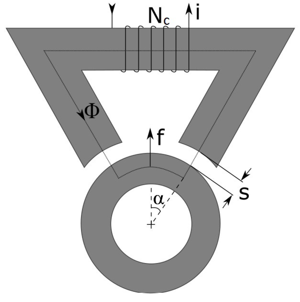
2.1. Basic Theory of AMBs

The reluctance force-based classic active magnetic bearing can be considered a typical mechatronic product with different components. Figure 1 illustrates the interaction of the components of an active magnetic bearing system. The controller receives the error ϵ of the rotor’s displacement and sends a reference current signal i * to the current controller to counteract the error and correct the rotor’s position. The current controller then realises the voltage u on the coils, resulting in a flowing current that generates a magnetic field. This magnetic field affects the rotor and its position in the mechanic plant. The measured position x m is then fed back to the controller and compared to the reference displacement x * .
In a classical radial AMB configuration, the rotor is supported by two radial bearings, which can be simplified to a four-phase horseshoe-shaped electromagnet, as illustrated by Figure 2. The currents in coils are denoted as i x + and i x for the current in the coil in the positive and negative x direction, respectively. The notation in y direction follows the same pattern. Compared to a three-phase approach, the control is simplified because forces can be generated in either positive or negative x and y direction. Further, the four-phase approach allows the easy utilisation of the differential driving mode, explained in the following paragraph.
Each phase can generate a magnetic flux Φ and a force f dependent on several constants, such as the permeability of vacuum μ 0 , the number of windings N c , the cross-section A of the electromagnet leg and the angle between legs α . Moreover, it is influenced by the air gap size s and the current i flowing in the coil, as shown in Figure 3.
The force f can be expressed by:
f = 1 4 μ 0 N c 2 A i 2 s 2 cos ( α ) ,
and can be simplified with
f = k i 2 s 2 w i t h k = 1 4 μ 0 N c 2 A cos ( α ) .
The last equations depend on current i squared, which means that the sign of the current applied on the coils can be neglected. Only the amplitude influences the force.
A common way to implement AMBs control is the so-called differential driving mode, in which each electromagnet works with an opposing one. In the case of the Y-axis, the force f y represents the difference between the top and bottom electromagnet, f y + and f y :
f y = f y + f y .
The top electromagnet is driven with the sum of the bias current i 0 and the control current i y . The opposite electromagnet, instead, is driven by their difference. By inserting Equation (2) into Equation (3) and setting ( i 0 + i y ) = i and ( s 0 y ) = s for the upper magnet and ( i 0 i y = i ) and ( s 0 + y ) = s for the lower magnet, respectively, it yields to:
f y = k ( i 0 + i y ) 2 ( s 0 y ) 2 ( i 0 i y ) 2 ( s 0 + y ) 2 .
Here, y denotes the displacement of the rotor in y direction. Equation (4) can be simplified and linearised with respect to small displacements compared to the air gap size ( x < < s 0 ):
f y ( y , i ) = k i i y k s y ,
with
k i 4 k i 0 s 0 2 a n d k s 4 k i 0 2 s 0 3 .
According to this equation, the driving of the rotor position can only be realised with the control current i y . The same method can be applied to the X-axis analysis and yields the same result.

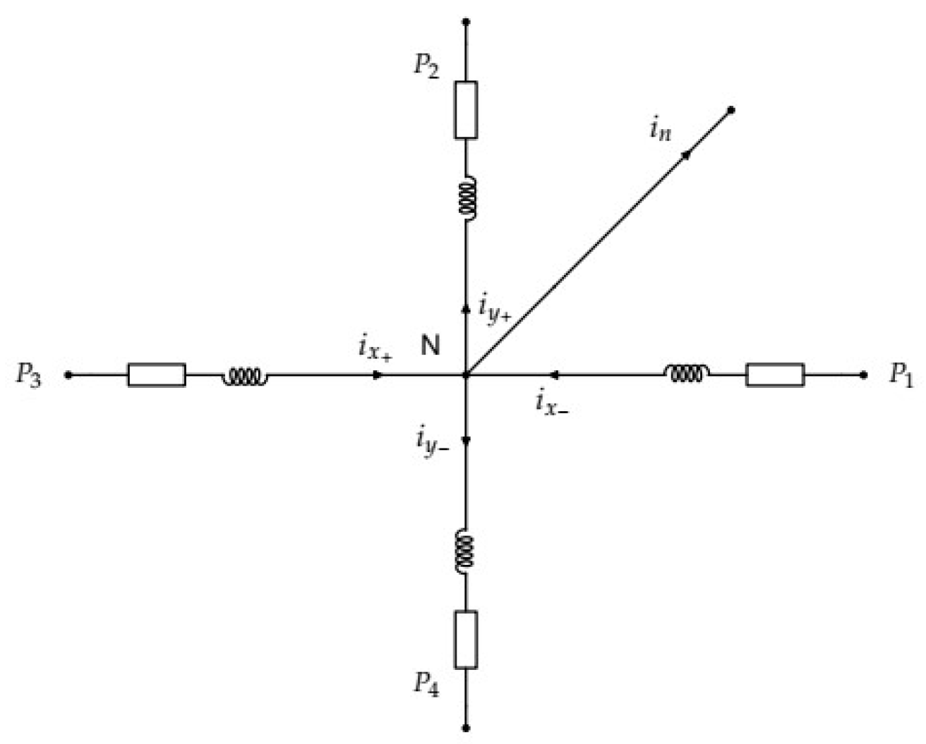
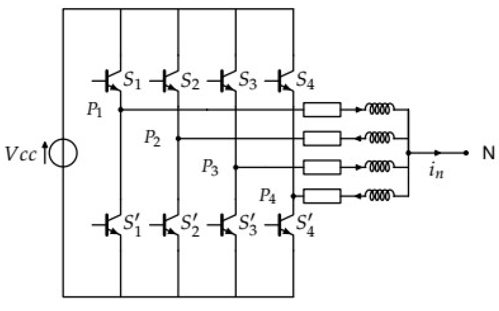
2.2. Proposed Driving Method with Star Connection

2.2.1. For Four-Phase AMB Topology

In order to realise the differential driving mode, 4 phase currents, i x + , i y + , i x and i y , are needed. They are individually composed of 2 variables: a bias current i 0 , which is identical for all phases, and a control current i x or i y , respectively. They can be mathematically expressed as:
i x + = i 0 + i x a n d i x = i 0 i x ,
i y + = i 0 + i y a n d i y = i 0 i y .
A star connection of 4 phases is realised by interconnecting the four coils, as illustrated in Figure 4. The common node N is the star point or neutral point. The current must be neutral at this node to obtain a stable system. According to Kirchoff’s current law, the current i N flowing through the star point is equal to the sum of all the other currents:
i N = k = 1 n i k = 0 .
Figure 4 and Equation (10) show a possible configuration that allows a stable operation regarding the phase currents in Equations (7) and (8), respectively. According to Equation (2), this is only possible because of the current flow’s sign, which does not affect the force generated by a phase.
i N = i x + + i x i y + i y = 0 .
This configuration with negative currents in y direction i y + and i y can be summarised by the matrix T D and its inverse T D such as:
i x + i y + i x i y = 1 0 1 1 0 1 1 1 1 0 1 1 0 1 1 1 T D i x i y i 0 i N ; i x i y i 0 i N = 1 4 2 0 2 0 0 2 0 2 1 1 1 1 1 1 1 1 T D i x + i y + i x i y .
With the star point i N = 0 , the transformation matrices can be simplified as:
T D = 1 0 1 0 1 1 1 0 1 0 1 1 ; T D = 1 4 2 0 2 0 0 2 0 2 1 1 1 1 .
These matrices allow the closed-loop control of the currents in the plant. The currents are composed of the bias current and the control currents i x and i y , as shown by the block diagram in Figure 5. The current errors, ϵ i x , ϵ i y and ϵ i 0 , are fed into three PI controllers, tuned according to the modulus optimum criterion [24]. In control theory, the modulus optimum criterion is a design principle that optimises the controllers’ behaviour in terms of the settling time [24]. With the help of the matrix T D , the resulting three output voltages are now transformed into four voltages which are then converted into PWM signals and applied to the circuit. The inverse matrix T D in the feedback loop provides the necessary backwards transformation.
Figure 6 shows a four-phase inverter that fulfils the earlier outlined requirements (star connection, four-phase, switching power amplifier). This kind of inverter is usually used for asynchronous and synchronous motors in star connection but with three phases instead. The transistors (Bipolar, MOSFET, etc.) of each phase S i and S i are complementary. When one is switched off, the other one is active. Therefore, the voltage outputs could be positive or negative. Currents can be generated depending on the differences between the duty cycles of the phases. The PWM duty cycles are centred at 50%. During functional operation with the developed method, two currents are positive and the two others negative. Therefore, two duty cycles are over 50%, while the two others are below 50%, which allows current generation.

2.2.2. For 4n-Phase AMB Topology

This method can be generalised for different applications. On the one hand, the addition of phases onto a radial bearing allows a better resolution or control of the magnetic flux resulting in a better dynamic of the rotor position. On the other hand, devices with several four-phase bearings, radial or axial, can get their neutral point connected to reduce the number of measurement devices using star-point current or voltage. These circuits are illustrated in Figure 7. However, the developed method was balanced for 4 phases and can only be generalised for 4n phases.
In this case, 4 n phases can drive 2 n axis. Therefore, there are 4 n phase currents composed of 2 n control and one bias current. It leads to Equation (13) and to the ( 4 n ) × ( 2 n + 1 ) transformation matrix T n . Its pseudo-inverse matrix T n is introduced in Equation (14) and can be used to deduce the control and bias currents from the phase currents. Both matrices can be used to convert currents and voltages as well.
i 1 + i 2 n + i 1 i 2 n = 1 1 1 O 1 O 1 1 1 1 1 1 1 O 1 O 1 1 1 1 T n i 1 i 2 n i 0
i 1 i 2 n i 0 = 1 2 1 2 1 2 1 2 O O 1 2 1 2 1 2 1 2 1 4 n 1 4 n 1 4 n 1 4 n T n i 1 + i 2 n + i 1 i 2 n
The following equations show the derivation of the coefficients of the matrices T n and T n , which allow quick and easy computation of the matrices. As expected, all the phase currents with odd indices are positive, and the phase currents with even indices are negative.
i [ 1 , 2 n ] , j [ 1 , 4 n ] ,
For T n :
t ( i , i ) = ( 1 ) i 1 ; t ( 2 n + i , i ) = ( 1 ) i ; t ( j , 2 n + 1 ) = ( 1 ) i 1 .
For T n :
t ( i , i ) = ( 1 ) i 1 2 ; t ( i , 2 n + 1 ) = ( 1 ) i 2 ; t ( 2 n + 1 , j ) = ( 1 ) i 1 4 n .
For increasing the magnetic flux resolution, the number of phases can be increased. Hereby, θ denotes the angle between the phases, for instance, 90 degrees in the case of a four-phase AMB. In order to simplify the control in such a case, a transformation matrix can be used:
i 1 i 2 n i 0 = c o s ( θ 1 ) s i n ( θ 1 ) 0 c o s ( θ 2 n ) s i n ( θ 2 n ) 0 0 0 1 i i x i i y i 0
in which, k [ 1 , 2 n ] ,
θ k = ( k 1 ) π 2 n .
Its inverse is:
1 n c o s ( θ 1 ) 1 n c o s ( θ 2 n ) 0 1 n s i n ( θ 1 ) 1 n s i n ( θ 2 n ) 0 0 0 1

3. Simulative Validation

3.1. Simulation Model and Parameters

The proposed driving method was tested numerically in a Matlab/Simulink model. Inspired by the block diagram in Figure 1, it easily allows testing different driving currents and position estimation methods with several plant designs. The focus of this work is on the validation of the proposed star connection, whereas the position control follows a known pole placement approach [1]. Figure 8 shows that a cascading control design has been chosen. The newly introduced PID position controller takes the error ϵ and calculates the desired current i * to counteract the error. In the current controller and power amplifier block, the desired currents are realised in the coils, represented by a physical model. The model utilises the prior introduced differential driving method. The now obtained actual currents in the coils are then fed into the AMB block. With the help of a physical representation of the plant, the forces and rotor position are calculated and fed back to the position controller. The position controller and the model of the plant are here duplicated in order to extend Figure 1 to a complete two-degrees-of-freedom (DOF) model.
The star-connected current method is also compared with a driving one composed of H-bridges. As mentioned in the introduction, a star-connected driving approach might result in unsuitable current dynamics for an AMB application. The simulation allows the investigation of the influence of the phase currents on each other compared to where they are completely independent. Table 1 summarises the hardware parameters used during the simulations and experiments.
The gains of the current controllers are listed in Table 2 and have been tuned based on the modulus optimum. The PID controller gains are listed in Table 3.

3.2. Simulation Results

The simulation’s purpose is the numerical validation of the proposed driving method. The actual current in the coils should follow a current command sent by a PID position controller. Furthermore, a disturbance force is applied on both axes. As shown in Figure 9, the disturbance force follows a stair pattern:
  • Step 1 (from 0 to 0.33 s): the disturbance force f g 1 = m × g = 1.96 N with starting condition x 0 = 1.0 × 10 3 m and y 0 = 0.5 × 10 3 m;
  • Step 2 (from 0.33 to 0.66 s): f g 2 = 2 × f g 1 = 3.92 N;
  • Step 3 (from 0.66 to 1.0 s): f g 3 = 5.66 N the limit disturbance force that one axis of the star-connected AMB can bear.
Figure 10 and Figure 11 indicate the resulting displacements on both axes as well as the corresponding phase currents according to the applied forces over time. First, it can be noticed during the entire simulation that the differential driving mode works as intended. At the beginning of step one, the maximum control currents are necessary to bring the rotor to the desired position. Until the start of step 2, the displacements and the phase currents are settling at a certain value, allowing the rotor to settle around the reference position. In step 2, the force needed to counteract the disturbance is higher and the system reacts as expected. The phase currents are settling at a higher plateau to tackle the bigger force. In step 3, the same behaviour is noticed with a saturation of the currents because of the differential driving mode itself. The control currents are reaching their maximum or minimum limit set with the absolute bias current | i 0 | .
The plots in Figure 12, Figure 13 and Figure 14 allow a comparison of the displacements and the phase currents with another topology in which each phase is independently driven by an H-bridge. In this particular case, four H-bridges are needed. The simulations demonstrate that the star-connection driving delivers the same behaviour as the H-bridge driving in terms of displacements and phase currents. At a second glance, it becomes apparent that the star-connected approach shows a bigger displacement overshoot. However, the rise and settling times are nearly the same. As it can be expected, the currents in Figure 14 show a familiar behaviour. The current tends more towards overshooting with the star-connected approach compared to the H-bridge driving. Again, the rise and settling times are not affected. The H-bridge driving reacts faster to the changing disturbance forces, giving the overall system better dynamics. Consequently, this results in the mentioned overshoots in displacement. However, the maximum displacement difference between both cases is only 10 5 m which can be neglected.
In conclusion, the star-connected four-phase inverter works as intended and can be considered as efficient as a full H-bridge driving topology in terms of the rotor displacement and phase current dynamic, respectively, and the error of both.

4. Experimental Validation

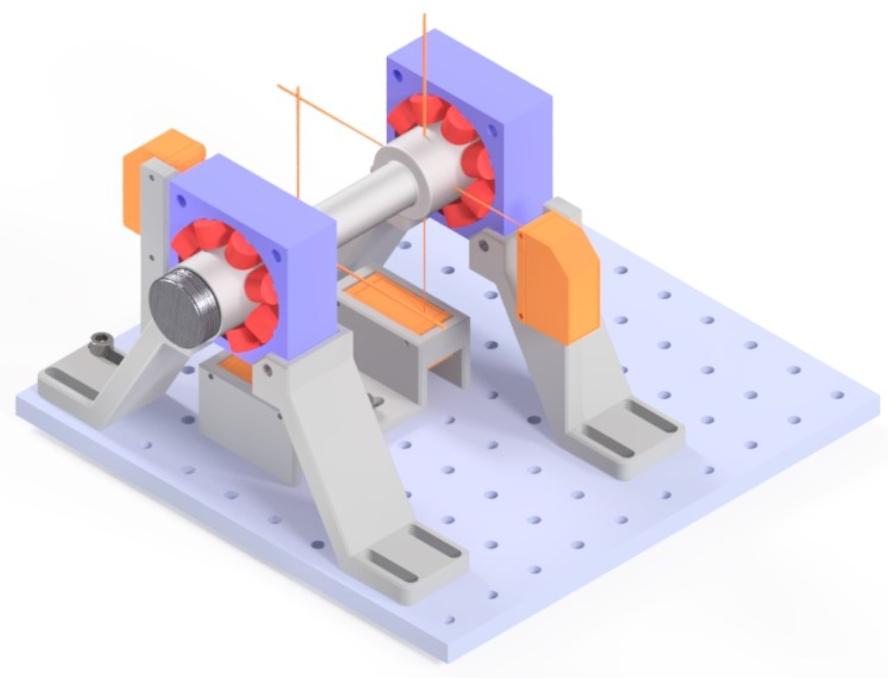
4.1. Experimental Setup

In order to evaluate the star-connected driving, an experimental test bench, shown in Figure 15, was set up. This test bench consists of two independent 2DOF magnetic bearings that stabilise the rotor in the X and Y direction. The axial shift in the z direction is neglected in this prototype application. Each bearing consists of an eight-pole stator with a heteropolar coil arrangement (blue). The eight coils (red) have 96 windings and are interconnected to pairs. The position of the rotor is measured by a total of four position sensors (orange) that operate at a sampling frequency of 2 kHz. The rotor is composed of an aluminium hull (light grey) and two ferromagnetic cores (darker grey), which are embedded in the hull at each end. This construction prevents a magnetic “sticking” in the event of a touchdown or in the startup phase. This design leads to a nominal mechanical air gap of 1 mm and a nominal magnetic air gap of 2 mm, meaning the outer aluminium hull has a thickness of 1 mm.
However, in this section, the focus will be on the currents and the proposed driving. The position control of the rotor is prototypical in this work and subject to further studies.
In order to realise the mentioned test bench, an electronic board and a mechanical plant are necessary. The electronic board, shown in Figure 16, was designed based on a 32-bit microcontroller and a four-phase MOSFET-based inverter. The microcontroller was chosen for its advanced-control timers, capable of generating pulse-width modulations (PWM) on six channels with a full modulation capability from 0 to 100%. The four-phase inverter operates at 36 V and was limited by the software to deliver a maximum phase current of 4 A and a bias current of 2 A. The measurements of the phase currents are conducted by four shunt amplifiers.
The experiment aims to check if the phase currents can follow an arbitrary input command. The profiles of the two control currents i x and i y are shown in Figure 17. The control current i x is a signal starting at 0 A with a step amplitude of 0.25 A each 0.5 s up to 1 A, from 0.5 s after the start of the experiment. The current i y is the same signal but negated and delayed by 1 s. Both are used in complement with the bias current of 2 A. According to Equations (7) and (8), the four desired phase currents are obtained. The positive currents i x + * , i x * and the negative currents i y + * , i y * are shown in Figure 18.

4.2. Experiment Results

Figure 19 shows the results of the experiments. The phase currents, i x + , i x , i y + and i y , follow the desired commands. During the experiment, the mean absolute error is below 0.7%. Some overshoots with an amplitude smaller than 0.2 A can be noticed at each step. Furthermore, the x and y currents influence each other but on a negligible scale. Figure 20 shows the back-transformed currents with small spikes at the switching instances of the reference current. Their absolute values are equal to the bias current of 2 A. As expected, the sum of all the currents equals zero, which means that the system is balanced. Thus, a successful implementation of the proposed star-point connection is achieved.
Because this work’s aim is to provide a star-connected power stage for a sensorless AMB operation, the inductances of the proposed circuit have been measured with an LCR meter. The measurements were conducted at 100Hz with the minimum and maximum air gaps of each axis, which is the closest and furthest rotor position away from the phases. Table 4 shows a heavy dependence on the position and inductance. These are promising results regarding the implementation of sensorless techniques.

5. Discussion and Conclusions

This work provides a new driving method for a four-phase active magnetic bearing that combines the classical differential driving mode with a star connection of the phases. Moreover, the method was generalised for 4 n phase actuators. It has been validated in a simulation and proved to be as efficient as full H-bridge driving. The method was tested experimentally with a custom-built four-phase inverter actuator. The results show that the phase currents were able to follow the reference signals with an average error of 0.7%. This new method gives new perspectives in the field of magnetic bearings and sensorless operation. The exploitation of the star connection with different methods is nowadays mostly employed in asynchronous or synchronous motors. The results of this work now allow the implementation of techniques like the DFC on AMBs. The future focus of interest will be on implementing more sophisticated position control strategies for star-connected AMBs. Building upon this, the implementation of sensorless position estimation techniques is of further interest.

Author Contributions

Conceptualisation, E.G., N.K. and R.B.; methodology, E.G., R.B. and N.K.; validation, R.B. and J.V.; formal analysis, N.K. and R.B.; software, R.B.; writing—original draft preparation, R.B., N.K. and J.V.; writing—review and editing, R.B., J.V., E.G., N.K. and M.N; funding acquisition, M.N. All authors have read and agreed to the published version of the manuscript.

Funding

This research received no external funding.

Institutional Review Board Statement

Not applicable.

Informed Consent Statement

Not applicable.

Data Availability Statement

Not applicable.

Acknowledgments

We acknowledge support by the Deutsche Forschungsgemeinschaft (DFG, German Research Foundation) and Saarland University within the funding programme Open Access Publishing.

Conflicts of Interest

The authors declare no conflict of interest.

Abbreviations

List of Symbols:
x * reference displacement in x direction
x m measured displacement in x direction
x 0 initial rotor displacement in x direction
y * reference displacement in y direction
y m measured displacement in y direction
y 0 initial rotor displacement in y direction
ϵ control error
ϵ i current error
uvoltage
icurrent
i 0 bias current
i N current in the star point
fforce
f g disturbance force
μ 0 permeability of vacuum
N c number of windings in a coil
Across-section area
α angle between the legs of the AMB
smagnetic air gap
T D inverse transformation matrix
T n generalised transformation matrix
T n inverse generalised transformation matrix
θ angle between the phases
Pphases
Stransistors
s 0 nominal magnetic air gap
Φ magnetic flux
kmachine constant
k i force/current factor
k s force/displacement factor
T D transformation matrix
List of Indices:
*control reference
xin x direction
yin x direction
+in positive direction
in negative direction

References

  1. Maslen, E.H.; Schweitzer, G. (Eds.) Magnetic Bearings: Theory, Design, and Application to Rotating Machinery; Springer: Berlin/Heidelberg, Germany, 2009. [Google Scholar] [CrossRef]
  2. Bleuler, H. A Survey of Magnetic Levitation and Magnetic Bearing Types. JSME Int. Journal. Ser. 3 Vib. Control. Eng. Eng. Ind. 1992, 35, 335–342. [Google Scholar] [CrossRef] [Green Version]
  3. Kucera, L. Robustness of Self-Sensing Magnetic Bearing. In Proceedings of the Magnetic Bearings Industrial Conference, Alexandria, VA, USA, 21–22 August 1997; p. 10. [Google Scholar]
  4. Noh, M. Self-Sensing Magnetic Bearings Driven by a Switching Power Amplifier. Ph.D. Thesis, University of Virginia, Charlottesville, VA, USA, 1996. [Google Scholar]
  5. Li, L.; Shinshi, T.; Shimokohbe, A. State Feedback Control for Active Magnetic Bearings Based on Current Change Rate Alone. IEEE Trans. Magn. 2004, 40, 3512–3517. [Google Scholar] [CrossRef]
  6. García, P.; Guerrero, J.M.; Briz, F.; Reigosa, D.D. Sensorless Control of Three-Pole Active Magnetic Bearings Using Saliency-Tracking-Based Methods. IEEE Trans. Ind. Appl. 2010, 46, 1476–1484. [Google Scholar] [CrossRef]
  7. Benjak, O.; Gerling, D. Review of position estimation methods for IPMSM drives without a position sensor part II: Adaptive methods. In Proceedings of the The XIX International Conference on Electrical Machines—ICEM 2010, Rome, Italy, 6–8 September 2010; IEEE: Rome, Italy, 2010. [Google Scholar] [CrossRef]
  8. Benjak, O.; Gerling, D. Review of Position Estimation Methods for PMSM Drives Without a Position Sensor, Part III: Methods based on Saliency and Signal Injection. In Proceedings of the 2010 International Conference on Electrical Machines and Systems, Incheon, Republic of Korea, 10–13 October 2010. [Google Scholar]
  9. Benjak, O.; Gerling, D. Review of position estimation methods for IPMSM drives without a position sensor part I: Nonadaptive methods. In Proceedings of the The XIX International Conference on Electrical Machines—ICEM 2010, Rome, Italy, 6–8 September 2010; IEEE: Rome, Italy, 2010. [Google Scholar] [CrossRef]
  10. Strothmann, R. Fremderregte Elektrische Maschine. EP Patent EP1005716B1, 14 November 2001. [Google Scholar]
  11. Mantala, C. Sensorless Control of Brushless Permanent Magnet Motors. Ph.D. Thesis, University of Bolton, Bolton, UK, 2013. [Google Scholar]
  12. Schuhmacher, K.; Grasso, E.; Nienhaus, M. Improved rotor position determination for a sensorless star-connected PMSM drive using Direct Flux Control. J. Eng. 2019, 2019, 3749–3753. [Google Scholar] [CrossRef]
  13. Werner, T. Geberlose Rotorlagebestimmung in Elektrischen Maschinen; Springer: Wiesbaden, Germany, 2018. [Google Scholar] [CrossRef]
  14. Grasso, E.; Mandriota, R.; König, N.; Nienhaus, M. Analysis and Exploitation of the Star-Point Voltage of Synchronous Machines for Sensorless Operation. Energies 2019, 12, 4729. [Google Scholar] [CrossRef] [Green Version]
  15. Grasso, E. Direct Flux Control—A Sensorless Technique for Star-Connected Synchronous Machines—An Analytic Approach; Shaker: Herzogenrath, Germany, 2021. [Google Scholar]
  16. Seiphetlho, T.E. Power Electronic Activation for Active Magnetic Bearings. Ph.D. Thesis, North-West University, Kirkland, WA, USA, 2006. [Google Scholar]
  17. Bartholet, M.T.; Nussbaumer, T.; Kolar, J.W. Comparison of Voltage-Source Inverter Topologies for Two-Phase Bearingless Slice Motors. IEEE Trans. Ind. Electron. 2011, 58, 1921–1925. [Google Scholar] [CrossRef]
  18. Jiang, D.; Li, T.; Hu, Z.; Sun, H. Novel Topologies of Power Electronics Converter as Active Magnetic Bearing Drive. IEEE Trans. Ind. Electron. 2020, 67, 950–959. [Google Scholar] [CrossRef]
  19. He, Y.; He, X.; Ma, J.; Fang, Y. Optimization Research on a Switching Power Amplifier and a Current Control Strategy of Active Magnetic Bearing. IEEE Access 2020, 8, 34833–34841. [Google Scholar] [CrossRef]
  20. Jiang, D.; Kshirsagar, P. Analysis and control of a reduced switch converter for active magnetic bearings. In Proceedings of the 2016 IEEE Applied Power Electronics Conference and Exposition (APEC), Long Beach, CA, USA, 20 March 2016; IEEE: Long Beach, CA, USA, 2016; pp. 3616–3622. [Google Scholar] [CrossRef]
  21. Hu, Z.; Jiang, D.; Sun, H.; Qu, R. A Shared-bridge Converter with Reversed Current Direction for Active Magnetic Bearing Drive. In Proceedings of the 2019 10th International Conference on Power Electronics and ECCE Asia (ICPE 2019—ECCE Asia), Busan, Republic of Korea, 27–31 May 2019; pp. 1–7. [Google Scholar]
  22. Hu, Y.; Yang, K.; Guo, X.; Zhou, J.; Wu, H. Evaluation of the Topology of Switching Power Amplifiers for Active Magnetic Bearings. Proceedings 2020, 64, 25. [Google Scholar] [CrossRef]
  23. Yang, J.; Jiang, D.; Sun, H.; Li, A.; Liu, Z. Series-winding Topology Converter for Active Magnetic Bearing Drive. IEEE Trans. Ind. Electron. 2020, 68, 11772–11782. [Google Scholar] [CrossRef]
  24. Schroeder, D. Elektrische Antriebe—Regelung von Antriebssystemen; Springer: Berlin/Heidelberg, Germany, 2015. [Google Scholar]
Figure 1. Block Diagram of Active Magnetic Bearing.
Energies 16 00396 g001
Figure 2. Classic radial four-phase AMB.
Energies 16 00396 g002
Figure 3. Force and geometry of a single AMB phase.
Energies 16 00396 g003
Figure 4. Equivalent circuit diagram of the proposed star connection.
Energies 16 00396 g004
Figure 5. Block diagram showing the described transformation and anti-transformation of the currents.
Energies 16 00396 g005
Figure 6. Equivalent circuit of the four-phase inverter model.
Energies 16 00396 g006
Figure 7. Possible equivalent circuitries for 8-axis bearings: (left) single radial bearing/(right) two radial bearings.
Energies 16 00396 g007
Figure 8. Block diagram of the simulated two-DOF bearing.
Energies 16 00396 g008
Figure 9. Profile of the disturbance force over time.
Energies 16 00396 g009
Figure 10. Displacements with the star connection.
Energies 16 00396 g010
Figure 11. Phase currents with the star connection.
Energies 16 00396 g011
Figure 12. Displacement comparison on x-axis.
Energies 16 00396 g012
Figure 13. Displacement comparison on y-axis.
Energies 16 00396 g013
Figure 14. Comparison of phase currents of both typologies.
Energies 16 00396 g014
Figure 15. Three-dimensional model of the test bench with stator (blue), coils (red), rotor (light grey), sensors (orange), supports (grey) and base plate (grey).
Energies 16 00396 g015
Figure 16. Motherboard used to drive the physical plant in the experiments.
Energies 16 00396 g016
Figure 17. Profile of the control current command.
Energies 16 00396 g017
Figure 18. Reference phase currents used in the experiment.
Energies 16 00396 g018
Figure 19. Measured phase currents before anti-transformation.
Energies 16 00396 g019
Figure 20. Measured bias and neutral current after anti-transformation.
Energies 16 00396 g020
Table 1. Hardware parameters.
ParameterSymbolValueUnit
Mass of the rotorm 2.0 × 10 1 kg
Nominal magnetic air gap s 0 2.0 × 10 3 m
Nominal mechanical air gap s m 0 1.0 × 10 3 m
Bias current i 0 2.5 A
Coil resistanceR 1.2 Ω
Coil inductanceL 2.18 × 10 3 H
Electromagnet factork 1.19 × 10 6 Hm
Force-displacement factor k s 316.16 N/m
Force-current factor k i 0.53 N/A
DC-link voltage for star-connected inverter u * 24V
DC-link voltage for H-bridges u H 12V
PWM frequency f A 2.0 × 10 4 Hz
Current sensor frequency f s 1.0 × 10 4 Hz
Table 2. Current controller gains.
GainSymbolValue
Proportional P P I 14.53
Integral I P I 6400
Table 3. Position controller gains.
GainSymbolValue
Proportional P P I D 5.0 × 10 3
Integral I P I D 8.0 × 10 4
Derivative D P I D 33.06
Filter coefficient N P I D 1000
Table 4. Measured inductances (in mH) on each phase at 100 Hz.
Phase x + x y + y
Minimum air gap2.181.841.872.09
Maximum air gap1.171.171.171.17
Disclaimer/Publisher’s Note: The statements, opinions and data contained in all publications are solely those of the individual author(s) and contributor(s) and not of MDPI and/or the editor(s). MDPI and/or the editor(s) disclaim responsibility for any injury to people or property resulting from any ideas, methods, instructions or products referred to in the content.

