

Usage of GAMS-Based Digital Twins and Clustering to Improve Energetic Systems Control

Abstract
:1. Introduction
1.1. Context
1.2. Literature Review
1.3. Contributions to Novelty
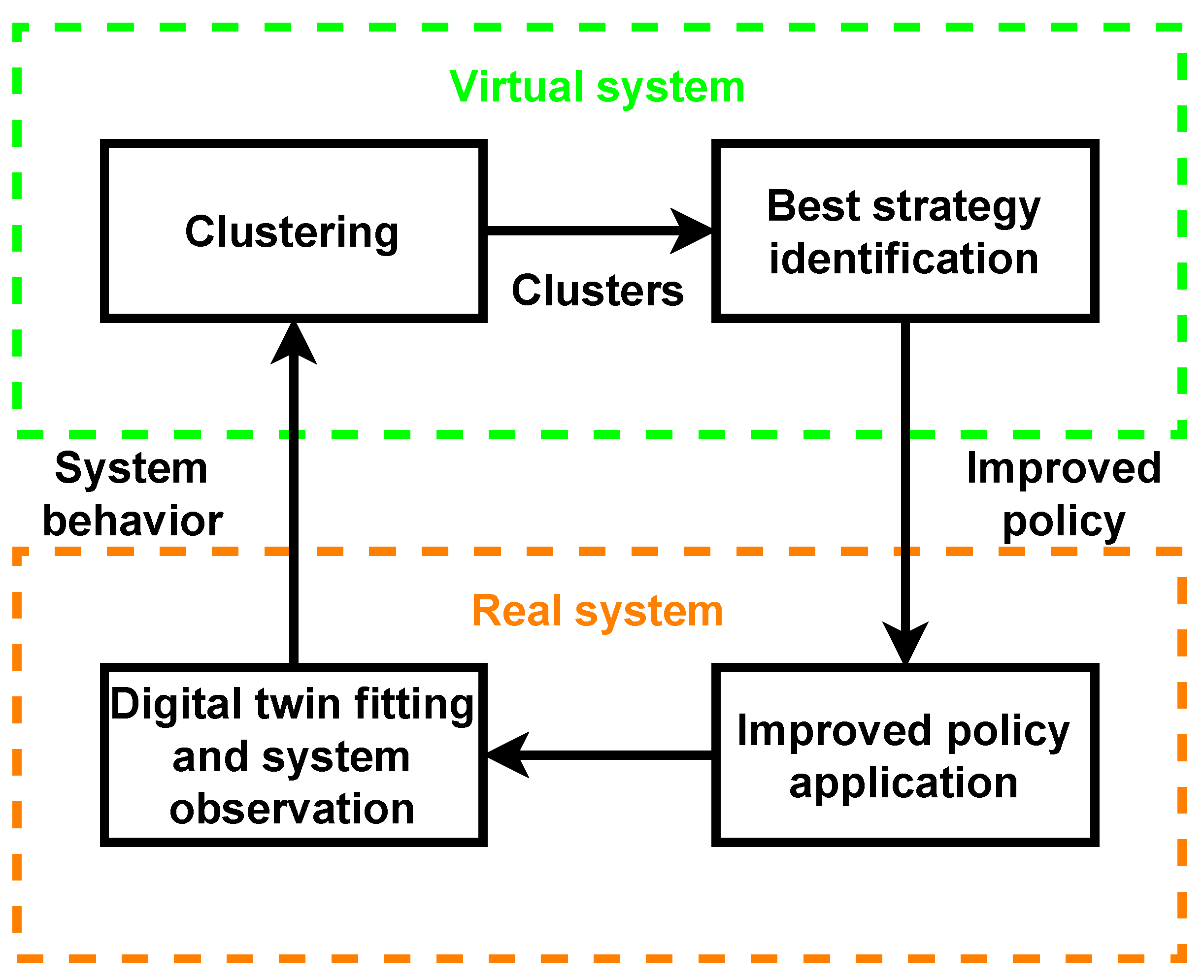
2. Methodology
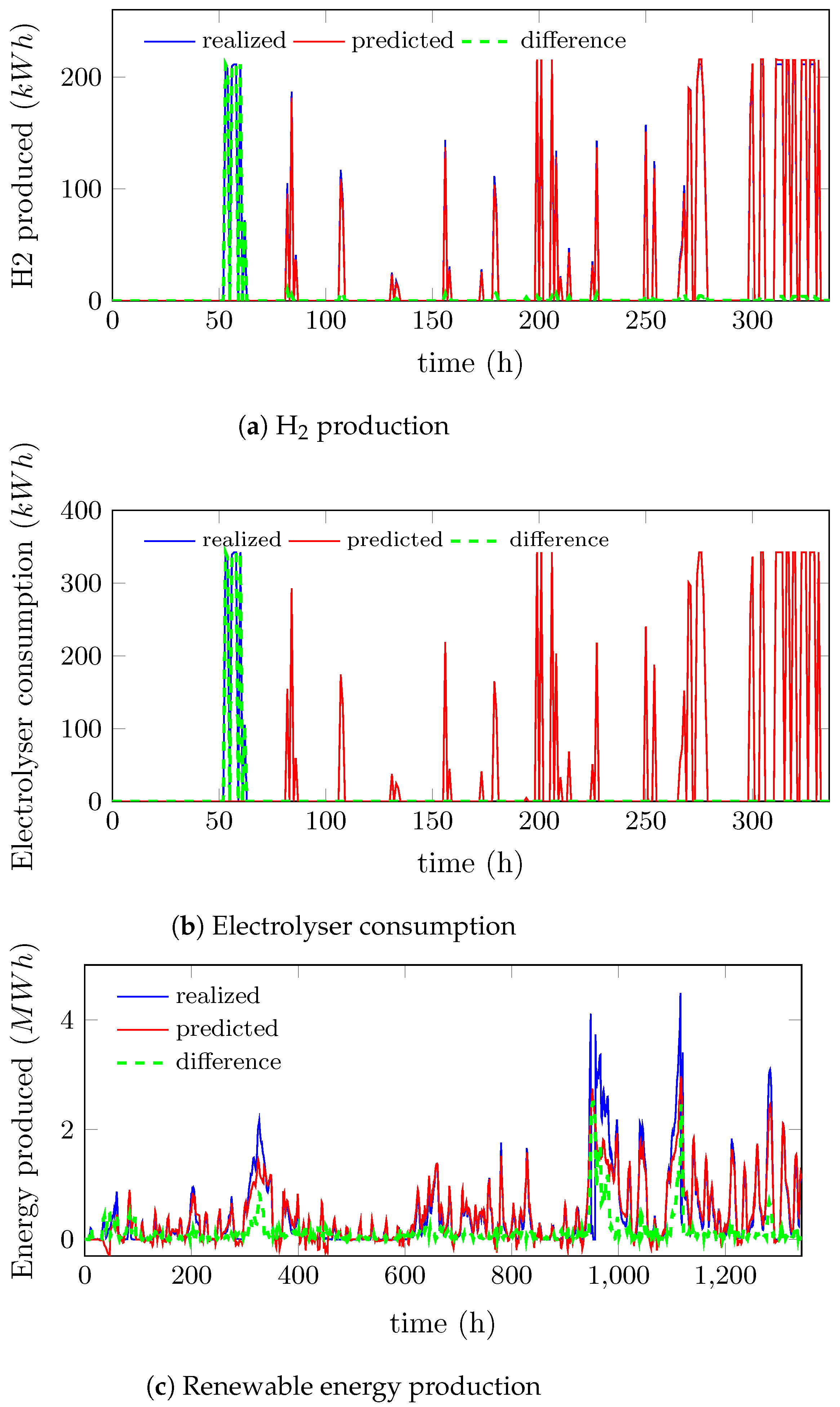
2.1. Digital-Twin Fitting and System Observation
2.2. Clustering
2.3. Policy Training
3. Case Study
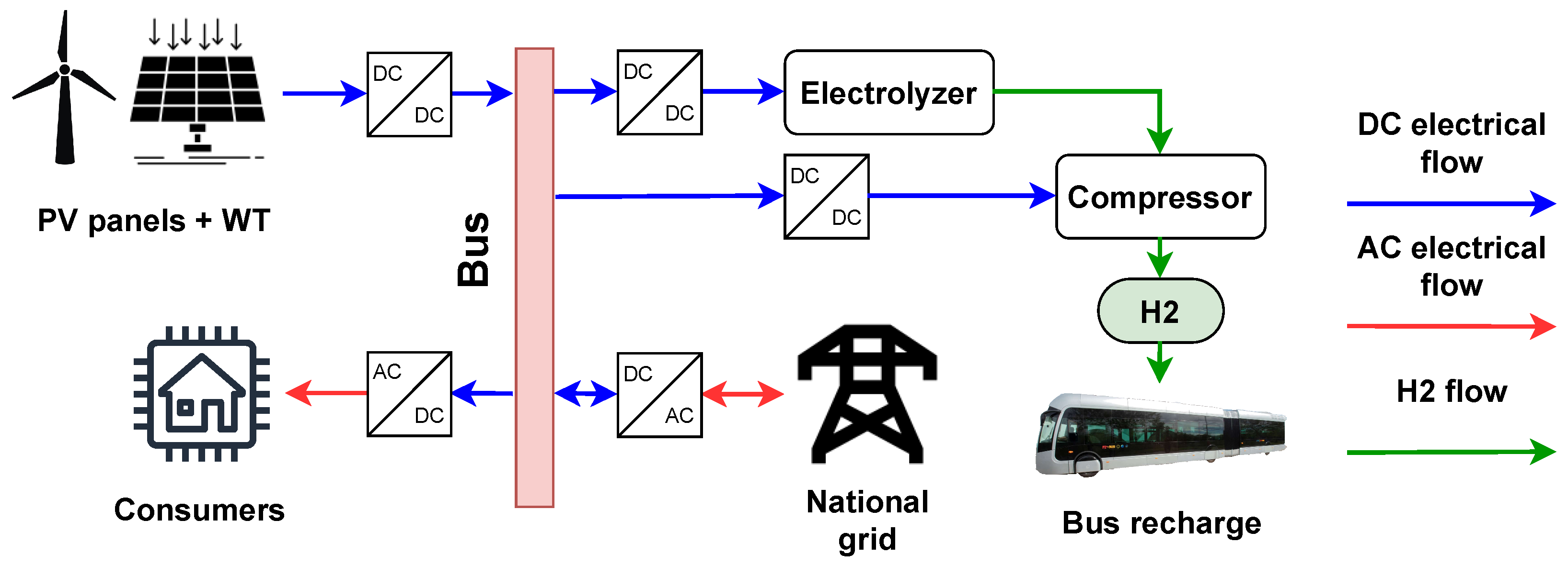
3.1. Description of the Microgrid
3.2. Additional Modeling Information
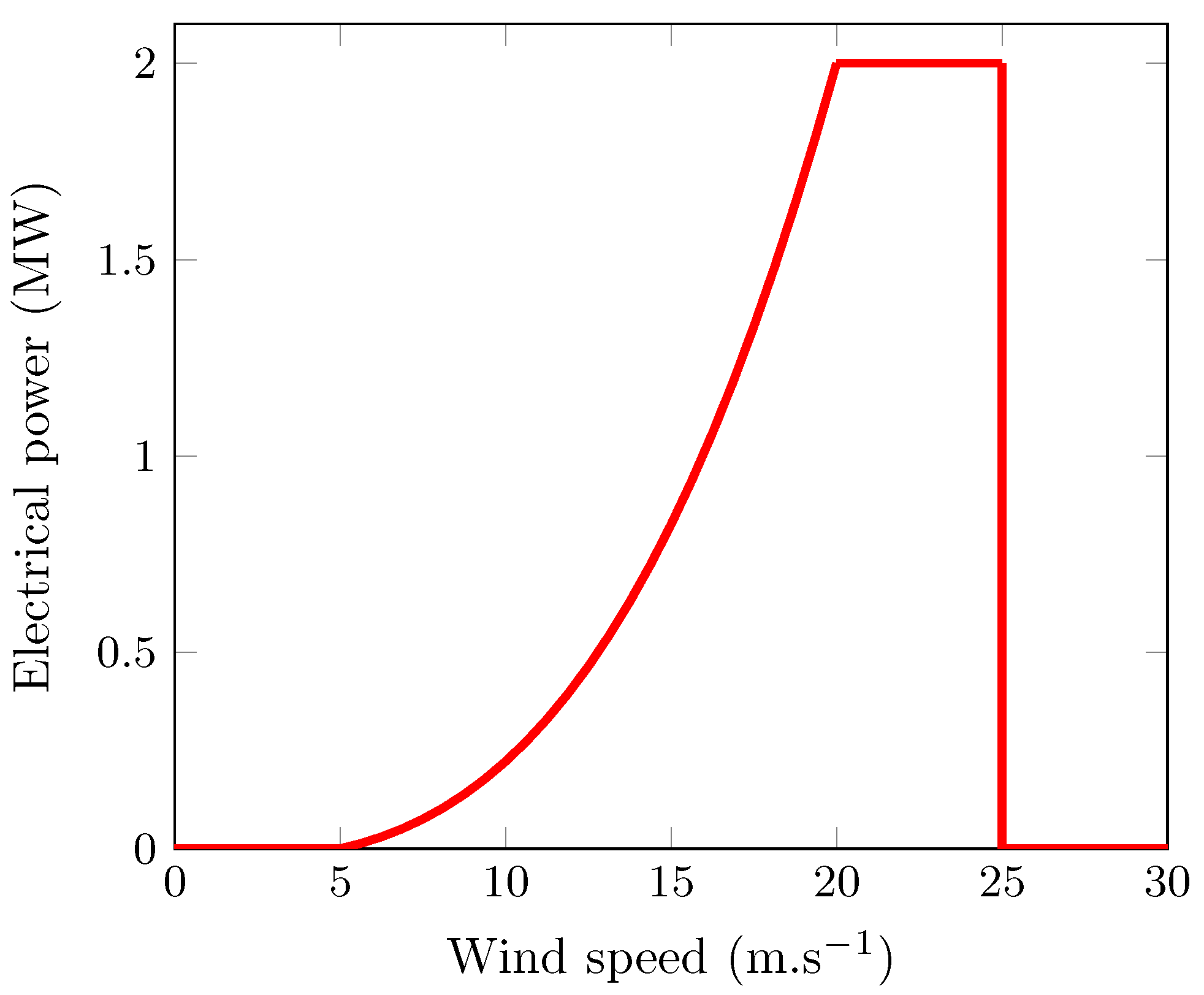
3.2.1. Wind Turbine
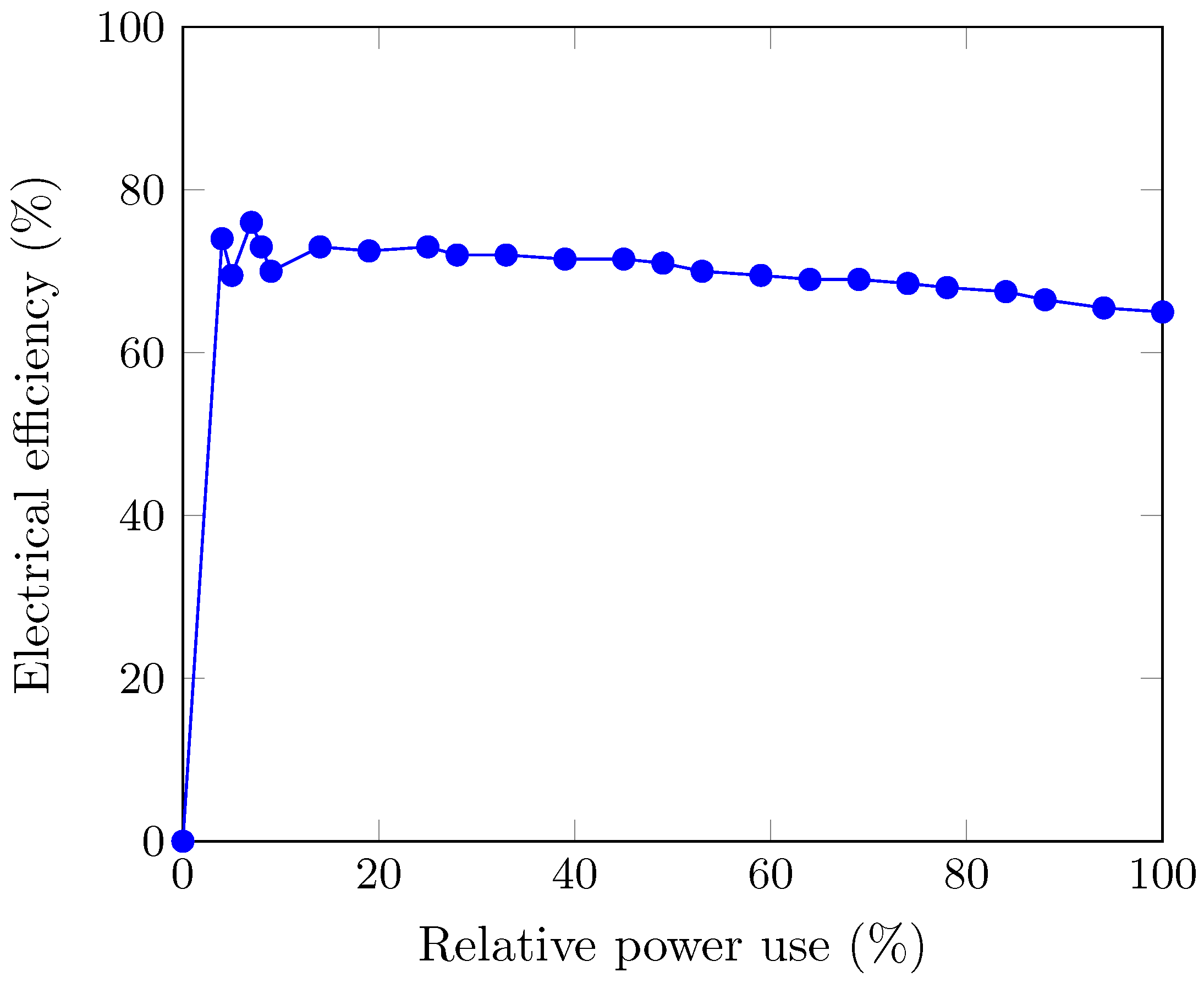
3.2.2. Electrolyser
3.2.3. Compressor
3.3. Sizing of the System
- Ninety houses, each house corresponding to 17 kW of solar power peak;
- An electrolyser of 325 kW;
- A tank accepting up to 1200 kg of hydrogen.
4. Method Implementation
4.1. Digital Twins Fitting
- Energy produced: given the meteorological state (irradiation, wind speed, temperature, ambient pressure), it returns the renewable energy production;
- H production: the H production for the total electricity consumed (electrolyser and compressor);
- Electrolyser consumption: for a total electricity used to produce H, this digital twin returns the consumption of the electrolyser branch. It is separated from the previous digital twin as it is needed to know which quantity to send in the electrolyser branch and in the compressor branch separately.
4.2. Control Strategies
| Algorithm 1 Storing strategy |
|
| Algorithm 2 Selling strategy |
|
4.3. Clustering
- Observe the system during one full year, as it can be considered as a complete cycle for meteorological and consumption variations;Concerning the prices, they have been quite unstable in Europe over the last year and it would be far beyond the scope of this article to make assumptions on their evolution. Thus, the one-year-long observation is considered good enough, as it contains at least the daily and seasonal variations;
- Replicate this single year of observation several times;
- Apply a Gaussian noise to the long sequence of several years.
- Energy available: the quantity of energy produced minus the consumption, i.e., the energy to be distributed between H production and electricity selling;
- Electricity price: the average electricity price over the sequence;
- H mass stored: the quantity of H available at the beginning of the session.
4.4. Policy Training
4.5. Performance Assessment
- Calculate the money earned if no H was produced and all electricity was sold to the grid;
- Sort the simulation rounds by increasing electricity prices;
- Calculate the total energy needed to produce H;
- Deduce the minimum loss, i.e., the minimum money not sold to the grid to the production of H;
- Calculate the theoretical best money flow by subtracting the money loss due to H production from the money earned when no H is produced;
- The over-performance is thus equal to the difference between the theoretical best money flow and the reference run money flow.
4.6. Simulation Plan
- Sequence length: the length of the sequences on which clustering is made;
- Standard deviation: the standard deviation used in the Gaussian noise applied to the clustering sequence;
- Relative weight of H production: the relative importance of H production when identifying the best strategy.
5. Results and Discussion
5.1. Digital Twins Fitting
5.2. Results of Policy Training
5.2.1. Overall Performance
5.2.2. Sensitivity to Parameters
6. Conclusions
Author Contributions
Funding
Data Availability Statement
Acknowledgments
Conflicts of Interest
Nomenclature
| Latin symbols | |
| A | surface area, |
| consumption, | |
| power coefficient, − | |
| c | specific heat capacity, |
| E | total energy, or |
| h | specific enthalpy, |
| l | length of a sequence in clustering, |
| lower heating value, or | |
| m | mass, |
| money flow, € | |
| molar mass, | |
| operational expenditures, € | |
| P | pressure, |
| power, | |
| production, | |
| price, € | |
| Q | heat, or |
| flow-rate, or | |
| R | individual ideal gas constant, |
| state of charge, % | |
| T | temperature, or |
| t | time, or min |
| V | volume, |
| Greek symbols | |
| ground roughness factor, − | |
| efficiency, − or % | |
| density, | |
| time constant, | |
| optimisation criterion, − | |
| Subscripts and superscripts | |
| air | |
| ambient | |
| bottom | |
| building | |
| charge | |
| cutoff | |
| discharge | |
| electrical | |
| Q | heat |
| heating | |
| inverter | |
| nominal | |
| outdoor | |
| panel | |
| reference | |
| Abbreviations | |
| DT | digital twin |
| EMS | energy management system |
| EPEX | european power exchange |
| GAMs | generalized additive models |
| ML | machine learning |
| photo-voltaic | |
| wind turbine |
References
- Mitali, J.; Dhinakaran, S.; Mohamad, A. Energy Storage Systems: A Review. Energy Storage Sav. 2022, 1, 166–216. [Google Scholar] [CrossRef]
- He, W.; King, M.; Luo, X.; Dooner, M.; Li, D.; Wang, J. Technologies and Economics of Electric Energy Storages in Power Systems: Review and Perspective. Adv. Appl. Energy 2021, 4, 100060. [Google Scholar] [CrossRef]
- A Hydrogen Strategy for a Climate-Neutral Europe; Technical Report; European Commission: Luxembourg, 2020.
- Vodovozov, V.; Raud, Z.; Petlenkov, E. Review of Energy Challenges and Horizons of Hydrogen City Buses. Energies 2022, 15, 6945. [Google Scholar] [CrossRef]
- Gronier, T.; Maréchal, W.; Gibout, S.; Geissler, C. Relevance of Optimized Low-Scale Green H2 Systems in a French Context: Two Case Studies. Energies 2022, 15, 3731. [Google Scholar] [CrossRef]
- Petrozziello, A.; Troiano, L.; Serra, A.; Jordanov, I.; Storti, G.; Tagliaferri, R.; La Rocca, M. Deep learning for volatility forecasting in asset management. Soft Comput. 2022, 26, 8553–8574. [Google Scholar] [CrossRef]
- Christensen, K.; Siggaard, M.; Veliyev, B. A Machine Learning Approach to Volatility Forecasting. 2021. Available online: https://papers.ssrn.com/sol3/Delivery.cfm/SSRN_ID3766999_code414727.pdf?abstractid=3766999&mirid=1 (accessed on 29 October 2022).
- Sadaqat, A.; Zheng, Z.; Aillerie, M.; Péra, M.C.; Hissel, D. A Review of DC Microgrid Energy Management Systems Dedicated to Residential Applications. Energies 2021, 14, 4308. [Google Scholar]
- Sang, J.; Sun, H.; Kou, L. Deep Reinforcement Learning Microgrid Optimization Strategy Considering Priority Flexible Demand Side. Sensors 2022, 22, 2256. [Google Scholar] [CrossRef]
- Nyong-Bassey, B.E. A Concise Review of Energy Management Strategies for Hybrid Energy Storage Systems. Eur. J. Eng. Technol. Res. 2022, 7, 77–81. [Google Scholar] [CrossRef]
- Arwa, E.O.; Folly, K.A. Reinforcement Learning Techniques for Optimal Power Control in Grid-Connected Microgrids: A Comprehensive Review. IEEE Access 2020, 8, 208992–209007. [Google Scholar] [CrossRef]
- Borden, K.; Herit, A.; Company, M. Digital Twins: What Could They Do for Your Business? 2022. Available online: https://www.mckinsey.com/capabilities/operations/our-insights/digital-twins-what-could-they-do-for-your-business (accessed on 1 August 2022).
- Rasheed, A.; San, O.; Kvamsdal, T. Digital Twin: Values, Challenges and Enablers from a Modeling Perspective. IEEE Access 2020, 8, 21980–22012. [Google Scholar] [CrossRef]
- Chinesta, F.; Cueto, E.; Abisset-Chavanne, E.; Duval, J.L.; Khaldi, F.E. Virtual, digital and hybrid twins: A new paradigm in data-based engineering and engineered data. Arch. Comput. Methods Eng. 2020, 27, 105–134. [Google Scholar] [CrossRef] [Green Version]
- Tao, F.; Xiao, B.; Qi, Q.; Cheng, J.; Ji, P. Digital twin modeling. J. Manuf. Syst. 2022, 64, 372–389. [Google Scholar] [CrossRef]
- Errandonea, I.; Beltrán, S.; Arrizabalaga, S. Digital Twin for maintenance: A literature review. Comput. Ind. 2020, 123, 103316. [Google Scholar] [CrossRef]
- Dembski, F.; Wössner, U.; Yamu, C. Digital twin. Virtual Reality and Space Syntax: Civic Engagement and Decision Support for Smart, Sustainable Cities. In Proceedings of the 12th International Space Syntax Conference, Beijing, China, 8–13 July 2019; pp. 8–13. [Google Scholar]
- Singh, M.; Fuenmayor, E.; Hinchy, E.P.; Qiao, Y.; Murray, N.; Devine, D. Digital twin: Origin to future. Appl. Syst. Innov. 2021, 4, 36. [Google Scholar] [CrossRef]
- Qi, Q.; Tao, F.; Hu, T.; Anwer, N.; Liu, A.; Wei, Y.; Wang, L.; Nee, A. Enabling technologies and tools for digital twin. J. Manuf. Syst. 2021, 58, 3–21. [Google Scholar] [CrossRef]
- Zheng, Y.; Yang, S.; Cheng, H. An application framework of digital twin and its case study. J. Ambient. Intell. Humaniz. Comput. 2019, 10, 1141–1153. [Google Scholar] [CrossRef]
- Lu, H.; Du, M.; Qian, K.; He, X.; Wang, K. GAN-based data augmentation strategy for sensor anomaly detection in industrial robots. IEEE Sens. J. 2021, 22, 17464–17474. [Google Scholar] [CrossRef]
- Gan, J.; Smith, C. Drivers for renewable energy: A comparison among OECD countries. Biomass Bioenergy 2011, 35, 4497–4503. [Google Scholar] [CrossRef]
- Lu, J.; Yi, S. Autoencoding Conditional GAN for Portfolio Allocation Diversification. arXiv 2022, arXiv:2207.05701. [Google Scholar]
- Xu, Y.; Sun, Y.; Liu, X.; Zheng, Y. A digital-twin-assisted fault diagnosis using deep transfer learning. IEEE Access 2019, 7, 19990–19999. [Google Scholar] [CrossRef]
- Maschler, B.; Braun, D.; Jazdi, N.; Weyrich, M. Transfer learning as an enabler of the intelligent digital twin. Procedia CIRP 2021, 100, 127–132. [Google Scholar] [CrossRef]
- Xia, M.; Shao, H.; Williams, D.; Lu, S.; Shu, L.; de Silva, C.W. Intelligent fault diagnosis of machinery using digital twin-assisted deep transfer learning. Reliab. Eng. Syst. Saf. 2021, 215, 107938. [Google Scholar] [CrossRef]
- Deebak, B.; Al-Turjman, F. Digital-twin assisted: Fault diagnosis using deep transfer learning for machining tool condition. Int. J. Intell. Syst. 2021, 1–28. [Google Scholar] [CrossRef]
- Liu, M.; Fang, S.; Dong, H.; Xu, C. Review of digital twin about concepts, technologies, and industrial applications. J. Manuf. Syst. 2021, 58, 346–361. [Google Scholar] [CrossRef]
- Naser, M. Digital twin for next gen concretes: On-demand tuning of vulnerable mixtures through Explainable and Anomalous Machine Learning. Cem. Concr. Compos. 2022, 132, 104640. [Google Scholar] [CrossRef]
- Jamal, S.; Tan, N.M.L.; Pasupuleti, J. A Review of Energy Management and Power Management Systems for Microgrid and Nanogrid Applications. Sustainability 2021, 13, 10331. [Google Scholar] [CrossRef]
- Battula, A.R.; Vuddanti, S.; Salkuti, S.R. Review of Energy Management System Approaches in Microgrids. Energies 2021, 14, 5459. [Google Scholar] [CrossRef]
- Boukas, I.; Ernst, D.; Théate, T.; Bolland, A.; Alexandre, H.; Martin, B.; Wynants, C.; Cornélusse, B. A deep reinforcement learning framework for continuous intraday market bidding. Mach. Learn. 2021, 110, 2335–2387. [Google Scholar] [CrossRef]
- Aittahar, S.; Manuel de Villena Millan, M.; Derval, G.; Castronovo, M.; Boukas, I.; Gemine, Q.; Ernst, D. Optimal Control of Renewable Energy Communities with Controllable Assets. 2022. Available online: https://hdl.handle.net/2268/264828 (accessed on 1 September 2022).
- Bolland, A.; Boukas, I.; Berger, M.; Ernst, D. ointly Learning Environments and Control Policies with Projected Stochastic Gradient Ascent. J. Artif. Intell. Res. 2022, 73, 117–171. [Google Scholar] [CrossRef]
- Henry, R.; Ernst, D. Gym-ANM: Reinforcement learning environments for active network management tasks in electricity distribution systems. Energy AI 2021, 5, 100092. [Google Scholar] [CrossRef]
- Yang, Y.; Li, H.; Shen, B.; Pei, W.; Peng, D. Microgrid Energy Management Strategy Base on UCB-A3C Learning. Front. Energy Res. 2022, 10, 858895. [Google Scholar] [CrossRef]
- Munos, R.; Stepletn, T.; Harutyunyan, A.; Bellemare, M.G. Safe and efficient off-policy reinforcement learning. Advances in Neural Information Processing Systems 29 (NIPS 2016). 2016. Available online: https://proceedings.neurips.cc/paper/2016/file/c3992e9a68c5ae12bd18488bc579b30d-Paper.pdf (accessed on 1 January 2019).
- Sutton, R.S.; Barto, A.G. Reinforcement Learning: An Introduction; The MIT Press: Cambridge, MA, USA, 2018. [Google Scholar]
- Rodrigues, C.; Gérard, P.; Rouveirol, C. On and Off-Policy Relational Reinforcement Learning. 2008. Available online: https://lipn.univ-paris13.fr/~gerard/docs/publications/rodrigues-ger-rou-ilp08-submit.pdf (accessed on 1 July 2017).
- LegiFrance. Articles L291-1 et L291-2 du code de l’énergie. 2021. Available online: https://www.legifrance.gouv.fr/codes/article_lc/LEGIARTI000043976710 (accessed on 1 November 2022).
- Dufo-López, R.; Bernal-Agustín, J.L.; Yusta-Loyo, J.M.; Domínguez-Navarro, J.A.; Ramírez-Rosado, I.J.; Lujano, J.; Aso, I. Multi-Objective Optimization Minimizing Cost and Life Cycle Emissions of Stand-Alone PV–Wind–Diesel Systems with Batteries Storage. Appl. Energy 2011, 88, 4033–4041. [Google Scholar] [CrossRef]
- Gelaro, R.; McCarty, W.; Suárez, M.J.; Todling, R.; Molod, A.; Takacs, L.; Randles, C.A.; Darmenov, A.; Bosilovich, M.G.; Reichle, R.; et al. The Modern-Era Retrospective Analysis for Research and Applications, Version 2 (MERRA-2). J. Clim. 2017, 30, 5419–5454. [Google Scholar] [CrossRef] [PubMed]
- Burton, T.; Jenkins, N.; Sharpe, D.; Bossanyi, E. Wind Energy Handbook, 2nd ed.; John Wiley & Sons, Ltd.: Hoboken, NJ, USA, 2011. [Google Scholar]
- Yue, M.; Lambert, H.; Pahon, E.; Roche, R.; Jemei, S.; Hissel, D. Hydrogen energy systems: A critical review of technologies, applications, trends and challenges. Renew. Sustain. Energy Rev. 2021, 146, 111180. [Google Scholar] [CrossRef]
- Pelikan, M. Bayesian optimization algorithm. In Hierarchical Bayesian Optimization Algorithm; Springer: Berlin/Heidelberg, Germany, 2005; pp. 31–48. [Google Scholar]
- Maréchal, W. Utilisation de Méthodes Inverses Pour la caractéRisation de matéRiaux à Changement de Phase (MCP). Ph.D. Thesis, Thèse de Doctorat de l’Université de Pau et des Pays de l’Adour, Pau, France, 2014. [Google Scholar]
- Walters, F.H. (Ed.) Sequential Simplex Optimization: A Technique for Improving Quality and Productivity in Research, Development, and Manufacturing; Chemometrics Series; CRC Press: Boca Raton, FL, USA, 1991. [Google Scholar]
- The Future of Hydrogen; Technical Report; International Energy Agency: Paris, France, 2019.
- IRENA. Hydrogen: A Renewable Energy Perspective; Technical Report; International Renewable Energy Agency: Abu Dhabi, United Arab Emirates, 2019. [Google Scholar]


| Sequence Length (h) | Standard Deviation (-) | Relative Weight of H Production (-) |
|---|---|---|
| 2, 3, 6, 12, 18, 24 | 0, 0.1, 0.2, 0.3 | 0, 0.25, 0.5, 0.75 |
| Sequence length (h) | 2 | 3 | 6 | 12 | 18 | 24 |
| Financial gain (k€) | 1.7 | 2.6 | 1.8 | 5.4 | 4.1 | 6.8 |
| Non-delivery (days/year) | 3 | 26 | 23 | 67 | 52 | 79 |
| Gain per undelivered H (€/kg) | 17.0 | 3.3 | 2.6 | 2.7 | 2.7 | 2.9 |
| Standard deviation | 0 | 0.1 | 0.2 | 0.3 |
| Financial gain (k€) | 6.7 | 1.4 | 1.6 | 5.2 |
| Non-delivery (days/year) | 77 | 13 | 18 | 59 |
| Gain per undelivered H (€/kg) | 2.9 | 3.8 | 3.0 | 2.9 |
| Stock coefficient | 0 | 0.25 | 0.5 | 0.75 |
| Financial gain (k€) | 13.1 | 1.8 | 0.01 | 0 |
| Non-delivery (days/year) | 151 | 16 | 0 | 0 |
| Gain per undelivered H (€/kg) | 2.9 | 3.7 | N/A | N/A |
Disclaimer/Publisher’s Note: The statements, opinions and data contained in all publications are solely those of the individual author(s) and contributor(s) and not of MDPI and/or the editor(s). MDPI and/or the editor(s) disclaim responsibility for any injury to people or property resulting from any ideas, methods, instructions or products referred to in the content. |
© 2022 by the authors. Licensee MDPI, Basel, Switzerland. This article is an open access article distributed under the terms and conditions of the Creative Commons Attribution (CC BY) license (https://creativecommons.org/licenses/by/4.0/).
Share and Cite
Gronier, T.; Maréchal, W.; Geissler, C.; Gibout, S. Usage of GAMS-Based Digital Twins and Clustering to Improve Energetic Systems Control. Energies 2023, 16, 123. https://doi.org/10.3390/en16010123
Gronier T, Maréchal W, Geissler C, Gibout S. Usage of GAMS-Based Digital Twins and Clustering to Improve Energetic Systems Control. Energies. 2023; 16(1):123. https://doi.org/10.3390/en16010123
Chicago/Turabian StyleGronier, Timothé, William Maréchal, Christophe Geissler, and Stéphane Gibout. 2023. "Usage of GAMS-Based Digital Twins and Clustering to Improve Energetic Systems Control" Energies 16, no. 1: 123. https://doi.org/10.3390/en16010123