Application of IIA Method and Virtual Bus Theory for Backup Protection of a Zone Using PMU Data in a WAMPAC System

Abstract

Many wide area monitoring, protection, and control (WAMPAC) systems are being deployed by grid operators to deal with critical operational conditions that may occur in power systems. Thanks to the real-time measurements provided by a set of distributed phasor measurement units (PMUs), different protection algorithms can be run in a central location. In this context, this article presents and validates a novel method that can be used as a backup protection for a selected area in a power system. It merges the integrated impedance angle (IIA) protection method with the theory of virtual buses in wide area electrical power systems. The backup protection works this way: once a fault is detected (pickup time), another delay (added to the pickup time) is defined in order to wait for the primary protection to act. If this does not happen, the algorithm generates its backup trip. The proposed method has been called the zone integrated impedance angle (Zone IIA). A real-time PMU laboratory has been used to test the proposed algorithm using a real-time digital simulator (RTDS). The algorithm has been programmed in a real-time automation controller (RTAC). It has been tested in two different simulated setups: first, a 400 kV transmission system, with and without the use of renewable energy sources (RES); second, a 150 kV submarine line between the Greece mainland and an island, which is currently the longest submarine alternating current connection in the world. The results obtained during the tests have yielded tripping times for area protection in the order of 48 ms, if no time delay is used between the fault detection and the trip order. According to the test results, the proposed method is stable, reliable, obedient, and secure, also with RES installed in the power system. Additionally, the method is selective, i.e., during the tests no trip was executed for external faults, no trip was executed in no-fault condition, and all the applied internal faults were detected and tripped correctly. Finally, the protection method is easy to implement. The method is also applicable to protection against short circuits in distribution systems. According to the trip times observed during the tests, it is clear that these algorithms are well suited to implement backup protections in transmission grids, even in scenarios with high penetration of renewable energies. Considering that backup trip times in transmission grids are usually set between 400 and 1000 ms, and that the actuation times obtained by the proposed algorithm are under 100 ms, the method is suitable for its use as a backup protection.

1. Introduction

The development of wide area protection schemes is a challenging task, due to the large amount of input data and the wide range of potential operation conditions of the grid. All these factors must be jointly considered for their correct implementation and good performance against perturbances in the system. This complexity is even higher in systems with high penetration of renewable energy sources (RES). In these cases, it is highly important that the protection scheme is easy to implement, requires the minimum number of setting parameters, is scalable when the power system grows, and is also safe and dependable in its behaviour.

Recently, it has been observed that the apparent impedance seen by the relays under very heavy loads may in some cases lead to undesired trips. Examples of this kind of event were observed during the 2003 blackout in the United States and Canada [1], the 2003 blackout in Southern Sweden and Eastern Denmark [2], and the 2006 blackout in Europe [3,4]. This phenomenon is especially noticeable in the case of long transmission lines or Zone 3 elements that must provide backup protection for lines outgoing from substations with significant infeed. This situation is quite dangerous when wide area disturbances occur and may result in quick deterioration and a partial blackout of the system.

In this context, synchrophasor technology provides suitable tools to improve backup protection for wide area application. A phasor data concentrator (PDC/controller) in one single location can decide if there is a fault in the protected zone and, consequently, avoid unnecessary Zone 3 tripping caused by load encroachment [5]. Wide area monitoring, protection, and control (WAMPAC) systems include situational awareness applications that help system operators to deal with critical operational conditions that may occur in power systems. In WAMPAC systems, services like load generation balance, wide-area voltage stability, emergency frequency control, power oscillation detection, dynamic line rating, and islanding detection, among others, are usually implemented [5,6,7,8,9,10].

Typically, transmission systems are protected by differential relays (87) as primary protections, and distance relays as backup protections (21). In distribution systems the main protections are the overcurrent relays (50, 51, 67) but, with the increasing presence of renewable generation on the load side, this protection philosophy must change to a new one including differential relays, distance relays, and new protection algorithms specifically developed by this kind of power systems [11,12,13].

WAMPAC systems can also be employed for wide-area short-circuit protection. However, there is not much information in the literature related to this topic. Some research studies have proposed tools such as the integrated impedance angle (IIA) [14,15], which uses the positive sequence phasors of voltages and currents of the phasor measurement units (PMUs) installed at both ends of a line to protect it. It can be used in distribution and transmission systems to protect a two-terminal line. Another useful tool is the theory of the virtual bus [16] proposed as a step in the implementation of an algorithm able to calculate a wide-area voltage stability index.

The H2020 FARCROSS Project [17] is proposing and testing new protection algorithms that can be used in WAMPAC systems. In the context of this research project, this article proposes one of the algorithms that will be tested later in the real demonstrator which includes a set of connections between substations in Greece. Some of these connections are submarine cables between the mainland and Greek islands. In our case the proposed algorithm is based on a combination of the IIA with the theory of the virtual bus [16], with the main objective of operating as a backup protection for traditional schemes in wide-area protection schemes in transmission or distribution power systems. This protection scheme uses the time-synchronized positive sequence phasors of voltages and currents supplied by the PMUs based in Std. IEEE C37.118 [18]. It has the advantage that its settings are easy to be parametrized.

To evaluate the feasibility of the proposed protection scheme, it has been implemented, and then a battery of tests has been run in a laboratory setup using a real time digital simulator (RTDS) and real PMUs synchronized by a GPS signal. The protection algorithm has been programmed in a PDC and has been evaluated both as a line and as an area protection of transmission and distribution systems with RES.

All in all, the contribution of the present paper can be summarized as:

(1)

The proposal of a novel short circuit detection algorithm for zone protection, which can be integrated in a WAMPAC system. It is called the zone integrated impedance angle (Zone IIA), and it combines the IIA with the theory of the virtual bus.

(2)

The implementation of the algorithm with real hardware.

(3)

A set of tests including two scenarios: a 400 kV transmission system and a 150 kV submarine cable. In addition, the first scenario has been tested with and without the integration of RES.

Although the IIA method can be useful for a two-terminal line, the proposed algorithm has the advantage that it is able to protect a wider zone. Other advantages of the algorithm are that it is not affected by load encroachment and that it can be implemented in the central element of a WAMPAC system. Finally, it should be highlighted that the operation time is small enough to allow its use as a backup protection.

The structure of the article is as follows: Section 2 explains the integrated impedance angle protection method as described in [14,15], Section 3 explains the theory of virtual buses as described in [16], and in Section 4 the proposed Zone IIA method is explained. The test infrastructure used to validate the algorithm is described in Section 5. In Section 6 the proposed method is implemented in a 400 kV transmission system, whereas in Section 7 it is implemented in a 150 kV submarine transmission system. The results are discussed in Section 8, and conclusions are drawn in Section 9.

2. Integrated Impedance Angle Protection Scheme

The IIA protection method as described in [14,15] uses the positive sequence phasors of voltages and currents of PMUs installed at both ends of a line, as can be seen in Figure 1.

The positive sequence IIA is calculated using Equations (1) and (2), where $\widetilde{SII}$ is the positive sequence integrated impedance, and $\widetilde{V_{A+}}$, $\widetilde{V_{B+}}$, $\widetilde{I_{A+}}$, and $\widetilde{I_{B+}}$ are the positive sequence voltages and currents of both sides of the line, respectively.

$$\widetilde{SII}=\frac{\widetilde{V_{A+}}+\widetilde{V_{B+}}}{\widetilde{I_{A+}}+\widetilde{I_{B+}}},$$

(1)

$$IIA=arg\left(\frac{\widetilde{V_{A+}}+\widetilde{V_{B+}}}{\widetilde{I_{A+}}+\widetilde{I_{B+}}}\right),$$

(2)

The method proposed in [14] states that, when no-fault condition or external faults exist in the line, the angle of integrated impedance is within the range between 5° and 90°. In contrast, when an internal fault exists, the angle of integrated impedance is within −5° and −90° (see Figure 2).

The IIA method in [14] was proposed to protect lines with two terminals in distribution and transmission systems. In that study, the algorithm works just by supervising the angle of the positive sequence integrated impedance.

The main goal of the present study is to apply this method in a wide area protection scheme to work as backup protection of traditional protection schemes like line distance (21) or line differential protections (87L).

3. Theory of the Virtual Buses

The theory of the virtual buses was deeply described in [16] as a step in the implementation of an algorithm able to calculate a wide-area voltage stability index in the Korean power system.

For example, in the system shown in Figure 3, it is possible to define two virtual buses, one for the sending area and another for the receiving area.

The virtual buses can be calculated from PMU data obtained from each corridor line’s end as follows [16]:

$$\begin{gathered} \widetilde{I_{send}}=\sum \widetilde{i_{send,i}} , \\ \widetilde{I_{receive}}=\sum \widetilde{i_{receive,i}} , \end{gathered}$$

(3)

$$\begin{gathered} \widetilde{S_{send}}=\sum \widetilde{P_{send,i}}+j \sum \widetilde{Q_{send,i}} , \\ \widetilde{S_{receive}}=\sum \widetilde{P_{receive,i}}+j \sum \widetilde{Q_{receive,i}} , \end{gathered}$$

(4)

Using current ($\widetilde{I_{send}}$, $\widetilde{I_{send}}$) and complex power ($\widetilde{S_{send}}$, $\widetilde{S_{receive}}$), the virtual bus voltage ($\widetilde{V_{send}}$, $\widetilde{V_{receive}}$) can be calculated by dividing the complex power by the conjugate of the current [16]:

$$\begin{gathered} \widetilde{V_{send}}=\frac{\widetilde{S_{send}}}{\widetilde{I_{send}^{*}}} , \\ \widetilde{V_{receive}}=\frac{\widetilde{S_{receive}}}{\widetilde{I_{receive}^{*}}} , \end{gathered}$$

(5)

The method proposed in the present article merges this theory with the integrated impedance angle protection method in order to achieve a wide-area protection scheme based on PMU measurements.

4. Proposed Method

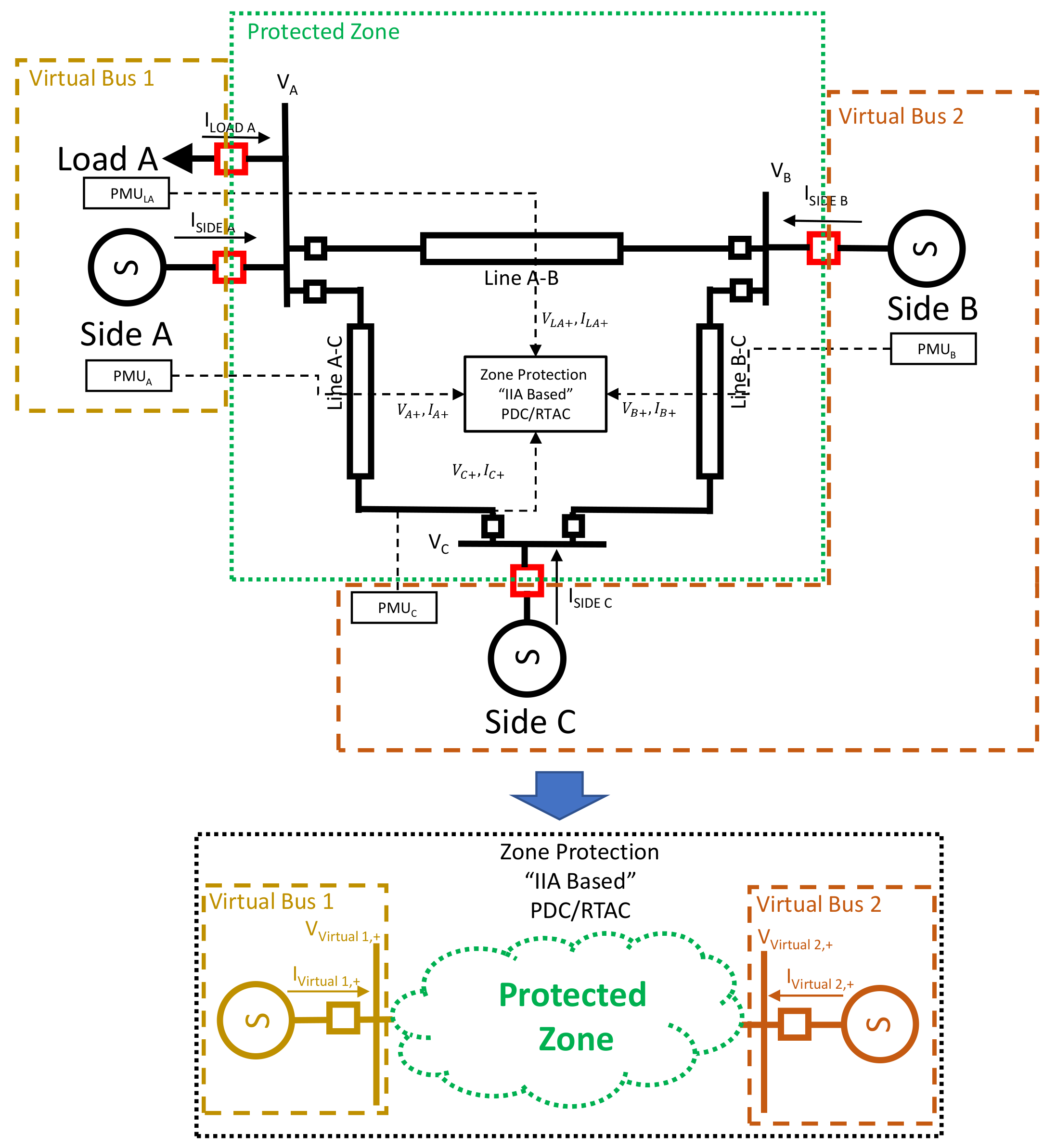
The proposed method merges the IIA protection scheme [14] with the application of the theory of the virtual bus [16] using the positive sequence phasors of voltages and currents measured by the PMUs located in the limits or the border and considering all power inputs and outputs of the zone to be protected. In Figure 4 a general scheme of the proposed method can be observed.

To calculate a positive sequence virtual bus, it is necessary to introduce the concept of apparent power in terms of symmetrical components. This relationship is explained in [19]:

$$\begin{gathered} \widetilde{S_{3Ø}}=\widetilde{V_a}\widetilde{I_a^{*}}+\widetilde{V_b}\widetilde{I_b^{*}}+\widetilde{V_c}\widetilde{I_c^{*}}=3\widetilde{V_a^{\left(0\right)}}\widetilde{I_a^{\left(0\right)*}}+3\widetilde{V_a^{\left(+\right)}}\widetilde{I_a^{\left(+\right)*}}+3\widetilde{V_a^{\left(-\right)}}\widetilde{I_a^{\left(-\right)*}} , \\ \widetilde{S_{3Ø}}=\widetilde{S_a}+\widetilde{S_b}+\widetilde{S_c}=\widetilde{S_{3Ø}^{\left(0\right)}}+\widetilde{S_{3Ø}^{\left(+\right)}}+\widetilde{S_{3Ø}^{\left(-\right)}}, \end{gathered}$$

(6)

The positive sequence apparent power ($\widetilde{S_{3Ø}^{\left(+\right)}}$) is considered, and the calculation of the virtual buses is defined as:

$$\widetilde{I_{VIRTUAL x}^{\left(+\right)}}=\sum \widetilde{i_{x,i}^{\left(+\right)}} ,$$

(7)

$$\widetilde{S_{VIRTUAL x}^{\left(+\right)}}=\sum 3·\widetilde{v_{x,i}^{\left(+\right)}}·\widetilde{i_{x,i}^{\left(+\right)*}},$$

(8)

$$\widetilde{V_{VIRTUAL x}^{\left(+\right)}}=\frac{\widetilde{S_{VIRTUAL x}^{\left(+\right)}}}{3·\widetilde{I_{VIRTUAL x}^{\left(+\right)}}},$$

(9)

where $i$ is the selected elements, part of the virtual bus $x$.

To apply the IIA method, it is necessary to define two virtual buses, as previously shown in Figure 4. The integrated impedance angle of the zone to be protected ($II{A}_{Zone}$) is defined as:

$$II{A}_{Zone}=arg\left(\frac{\widetilde{V_{VIRTUAL 1}^{\left(+\right)}}+\widetilde{V_{VIRTUAL 2}^{\left(+\right)}}}{\widetilde{I_{VIRTUAL 1}^{\left(+\right)}}+\widetilde{I_{VIRTUAL 2}^{\left(+\right)}}}\right),$$

(10)

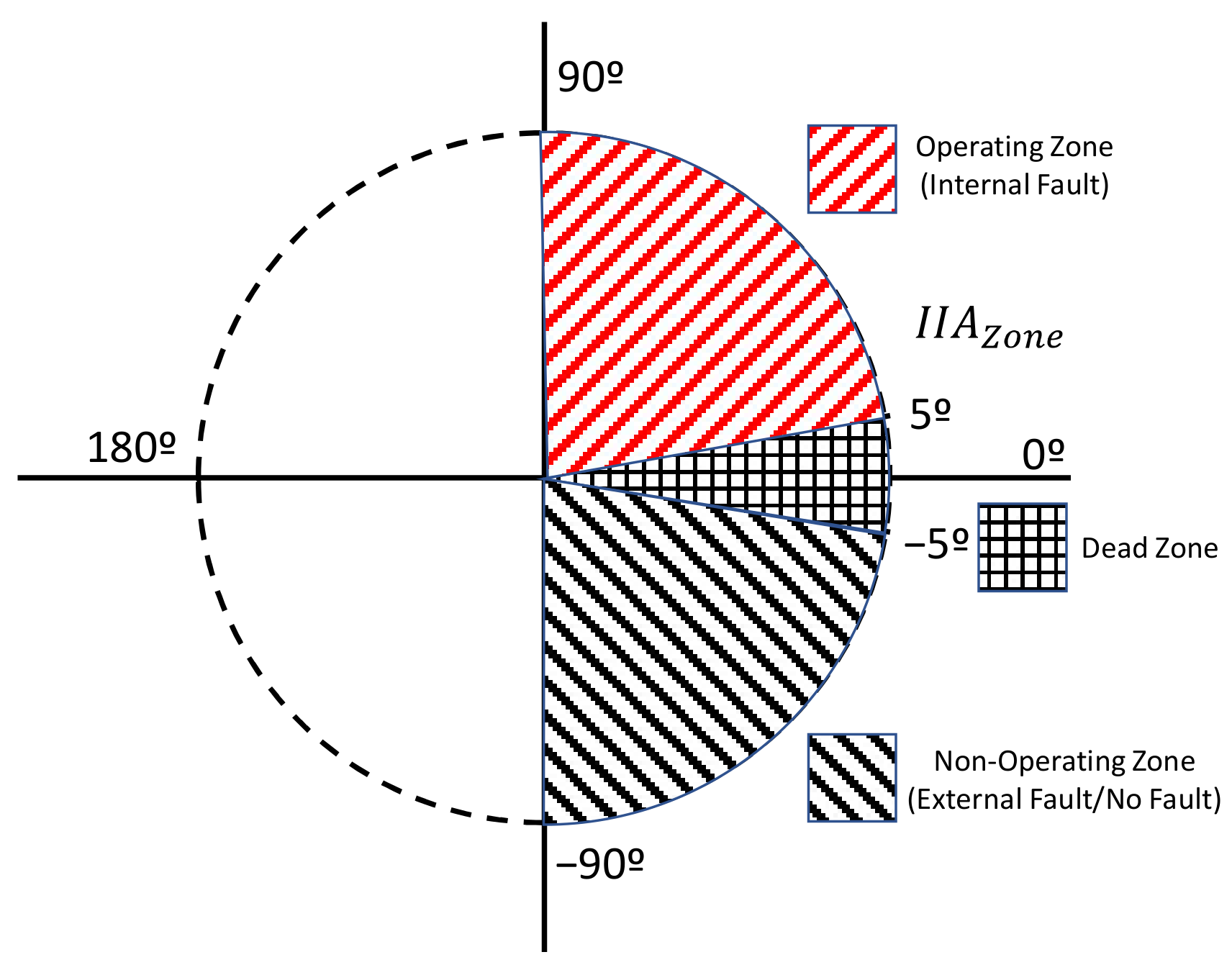
The operation characteristic associated with $II{A}_{Zone}$ is defined in Figure 5: when the angle of integrated impedance of the zone is within 5° and 90°, the algorithm declares that a fault condition exists inside the protected zone, and when the angle is within −5° and −90°, the algorithm declares that the fault is external or that no-fault condition exists.

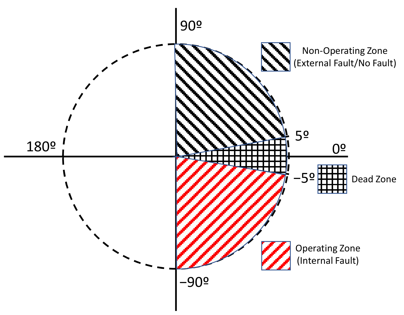
Note that the operating characteristic in Figure 5 is different from the one defined in Figure 2 [14]. The new operating characteristic was defined after observing the behaviour of the IIA angle scheme while protecting a line or a zone with different kinds of fault conditions. Internal zone faults result in a zone with an $II{A}_{Zone}$ angle between 5° and 90°, while external zone faults result in a zone with $II{A}_{Zone}$ between −5° and −90°. This behaviour will be further explained in Section 6 and Section 7.

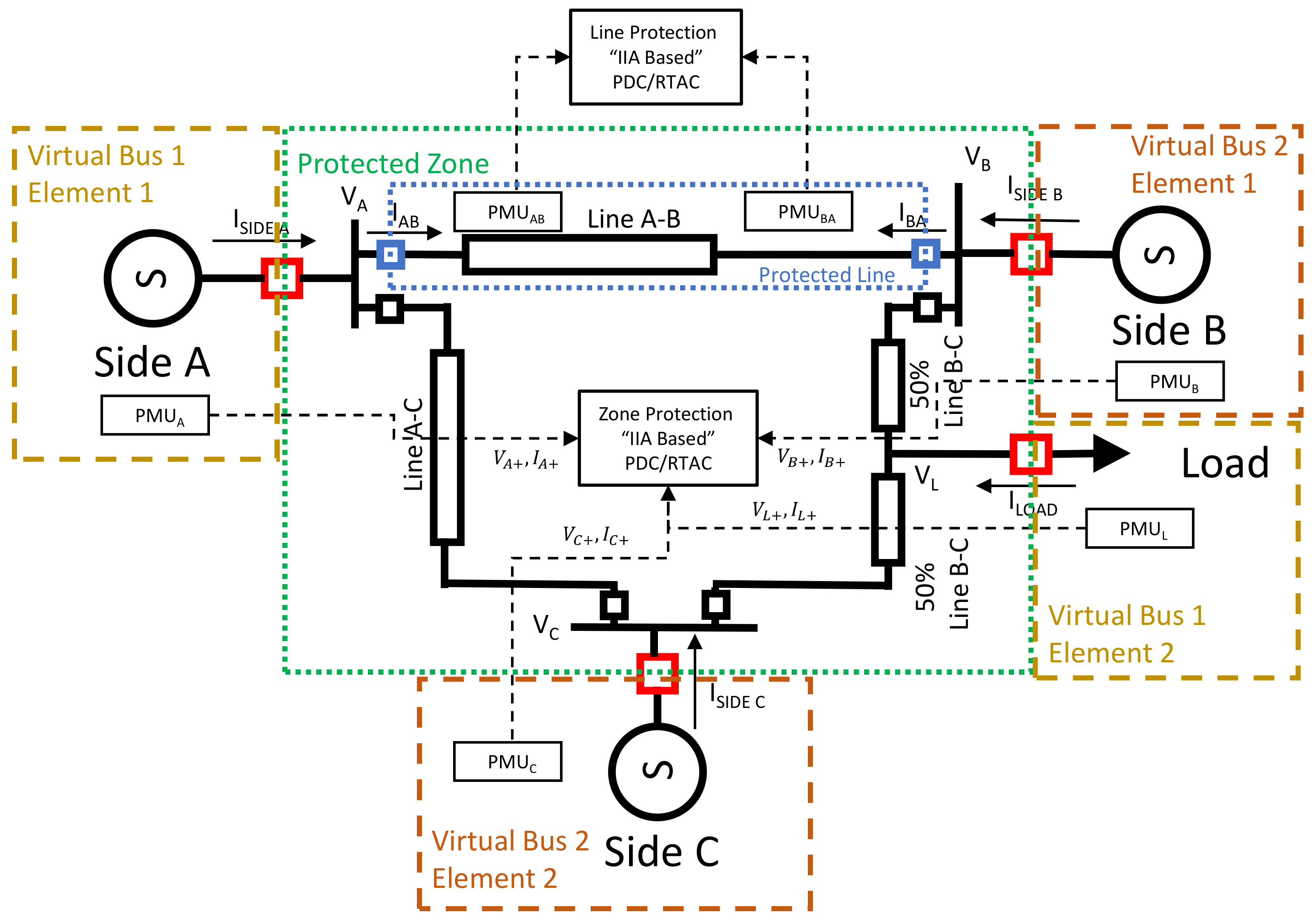
In Figure 6 the block diagram of the proposed method is represented. The first step of the method consists of defining the zone to be protected. Different criteria can be used to divide a large network into a number of zones; for example, the circuit breakers can be used as the elements that define the borders, since they provide the required isolation in case of a fault. Considering that the output of the algorithm is a potential trip, the zones should be small enough to limit the impact of the trip to the zone that is really affected by the fault. This is the reason why relatively small scenarios have been used in this study. The behaviour of the proposed method implemented in bigger power systems can be analysed in future works.

The next step is to distribute all the border elements of the selected zone to be protected into two groups. Each group has several PMUs associated with it wherein all data must be time-synchronized and with valid quality (i.e., the PMU has sent a measurement with a “Good” value in the “Validity” field according to IEEE C37.118) to proceed with the next steps. However, if “Validity” is “Invalid”, or if the data is not time-synchronized, the measurement is ignored for the next steps.

The next step consists of calculating the positive sequence virtual bus of each group, evaluating whether the data received is reliable or not, and checking the data quality and the time stamp of all the measurements. The constants $V_{valid}$ and $I_{valid}$ are set as thresholds to detect any anomalies in the measured magnitudes. They can be set as small as possible to ensure that the measurement received by PMUs is sufficient so as to consider it a valid measurement which can be included into the calculations of the method.

The next step encompasses the calculation of the $II{A}_{Zone}$. Two conditions must be accomplished to declare that an internal fault exists in the protected zone. The first one evaluates whether the magnitude of $\left|\widetilde{I_{VIRTUAL 1}^{\left(+\right)}}+\widetilde{I_{VIRTUAL 2}^{\left(+\right)}}\right|$ is bigger than a minimum polarization current ($I_{\min pol}$), and the second evaluates whether the $II{A}_{Zone}$ is between 5° and 90°. The minimum polarization current ($I_{\min pol}$) is defined in order to guarantee that the magnitude of the resulting current $\widetilde{I_{VIRTUAL 1}^{\left(+\right)}}+\widetilde{I_{VIRTUAL 2}^{\left(+\right)}}$ (the denominator of the integrated impedance of the protected zone) is big enough to present clear angle direction.

5. Testing Infrastructure

This section describes the real-time PMU laboratory used as the testing infrastructure. It has been built using the commercial devices typically used in these scenarios.

Real-Time PMU Laboratory

The laboratory includes three PMUs (two AXIONs from SEL, and one WAMSTER PMU-R1 from STER), an RTAC (SEL 3555), an industrial PC (SEL 3355), a communications switch (SEL-2730M), a GPS clock (SEL 2488), and an RTDS simulator including giga-transceiver analogue output (GTAO) and giga-transceiver network communication (version 2) with PMU firmware (GTNETx2-PMU) cards. All these elements are integrated in an infrastructure able to emulate and test any scenario in the grid. The RTDS can generate up to 8 additional PMUs and can simulate power system behaviour in real time.

In Figure 7, a diagram of the real-time PMU laboratory can be observed. In this setup, it is possible to use the RTDS to model electrical power systems that interact by means of hardware in the loop simulations, using real equipment, control systems, and electrical protection schemes. Therefore, it is a very convenient setup to test WAMPAC services and algorithms before their implementation in the field.

The RTDS allows one to simulate electrical power systems in real time. Using its giga-transceiver analogue output cards (GTAO), it is possible to convert signals, as voltages and currents generated in real time, into analogue signals that are sent to the amplifiers. The amplified signals of voltages and currents are connected to the analogue inputs of the physical devices, i.e., the AXION or WAMSTER PMUs.

The PMUs process their inputs and convert them into frames following the C37.118 protocol. The STER PMU creates a PMU server from which samples can be received by up to 4 clients at the same time. In the case of the SEL AXION, for each PMU client a PMU server must be configured. Using the GTNETx2-PMU card of the RTDS, it is possible to generate up to 8 additional PMU frames which can send voltages and current signals. Therefore, our lab setup results in a power system simulation in real time. The samples of each PMU generated by the RTDS can only be received by one client at a time.

The SEL-2488 GPS clock is responsible of distributing IRIG-B time synchronization signals to the RTDS, the SEL and STER PMUs, and the RTAC, in order to achieve time synchronization between all the elements of the laboratory.

The SEL-3555 RTAC works as a PDC and as a real-time controller. It can receive the PMU signals and process them. Different algorithms can be developed on it using IEC 61131-3 code [20,21,22]. The resulting remedial actions of the algorithms can be executed in the RTAC and communicated via IEC-61850 GOOSE messages to the AXIONs, which can operate their contact outputs, which can finally be detected by the RTDS (using its GTDI card) to close the loop. In addition, the RTAC and the RTDS communicate, so the latter can process IEC-61850 GOOSE messages and execute the remedial actions in real time over the simulated electrical power system. The RTAC SEL-3555 can also work also as a PMU server.

All the communications inside the PMU real-time laboratory pass through the Ethernet switch SEL-2730M. An industrial computer SEL-3355 is used to configure all the elements inside the laboratory. In [23] some additional capabilities of this real-time PMU laboratory were presented.

The fastest data rate established by the standard IEEE C37.118.2-2011 [18] for a 50 Hz power system is 50 frames per second (fps). The RTDS, the AXIONs, and the WAMSTER PMU-R1 can work with a data rate of 50 fps, i.e., one synchrophasor data frame every 20 milliseconds. The fastest process cycle rate used in the RTAC SEL-3555 to implement the proposed algorithm is one cycle each 1 ms. The PMU data is updated every 10 ms.

New developments in PMUs may achieve data frames faster than 50 fps, but for now they are not available in all the PMUs in the market. In addition, they are not required by IEEE C37.118.2-2011 [18,24,25].

Two power system scenarios are established to evaluate the behavior of the proposed method. The first is a 400 kV transmission grid, and the second is a 150 kV submarine one. The characteristics, tests and results corresponding to each scenario are presented in Section 6 and Section 7, respectively.

6. 400 kV Transmission Grid

This section describes the power system model used to test the proposed method in a 400 kV transmission grid with and without renewable energy resources. To evaluate the behaviour of the proposed method in this grid, the following scenario has been implemented (see Figure 8).

The electrical data of generators, transmission lines, and load can be found in

Table 1. Generator data for the 400 kV transmission system.

Generator Data	Side A	Side B	Side C
Nominal Voltage (kV)	400	400	400
Phase (deg)	0	15	20
Frequency (Hz)	50	50	50
Inductance Series + (Henry)	0.1	0.1	0.1
Resistance Series + (Ohm)	3.14	3.14	3.14
Inductance 0 Parallel (Henry)	0.1	0.1	0.1
Resistance 0 Parallel (Ohm)	3.14	3.14	3.14

,

Table 2. 400 kV transmission lines data.

Line AB, Line BC, Line CA
Model	Bergeron (RLC)
Line Length (km)	20
Positive Sequence Series Resistance (Ohm/km)	0.0293
Positive Sequence Series Ind. Reactance (Ohm/km)	0.3087
Positive Sequence shunt Cap. Reactance (MOhm·km)	0.2664
Zero Sequence Series Resistance (Ohm/km)	0.3
Zero Sequence Series Ind. Reactance (Ohm/km)	0.988
Zero Sequence Shunt Cap. Reactance (MOhm·km)	0.4369

and

Table 3. 400 kV load data.

Load
Active power (MW)	500
Reactive Power (MVAr)	309.9

, respectively.

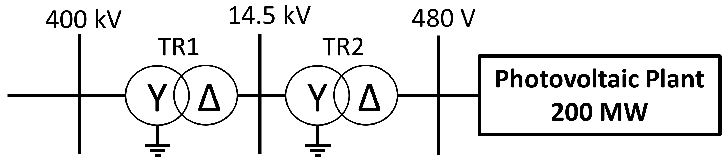
“Side B” can either be a generator with the characteristics shown in Table 1 or a Photovoltaic plant (Type D generator according to Spanish grid code [26]) generating 200 MW. Figure 9 represents the different parts of a photovoltaic plant.

In

Table 4. TR1 transformer data.

TR1
Apparent Power (MVA)	225
Frequency (Hz)	50
Leakage Inductance (p.u.)	0.15
No load losses (p.u.)	0.001
Winding 1 Voltage (kV)	400
Winding 1 Magnetizing current (%)	1
Winding 2 Voltage (kV)	14.5
Winding 2 Magnetizing current (%)	1

and

Table 5. TR2 transformer data.

TR2
Apparent Power (MVA)	225
Frequency (Hz)	50
Leakage Inductance (p.u.)	0.15
No load losses (p.u.)	0.001
Winding 1 Voltage (kV)	14.5
Winding 1 Magnetizing current (%)	1
Winding 2 Voltage (kV)	0.48
Winding 2 Magnetizing current (%)	1

, the electrical characteristics of TR1 and TR2 transformers are represented, respectively.

To evaluate the behaviour of the proposed method, different kinds of faults have been executed in different locations of the transmission system.

6.1. Tests Executed in the 400 kV Transmission Grid

In this section, the description of the executed tests to evaluate the behaviour of the proposed method is included. The different fault locations are represented in Figure 10.

Different types of internal line faults have been executed, namely A-G, B-G, C-G, AB, BC, CA, AB-G, BC-G, CA-G, ABC, ABC-G, with different fault resistances.

The definitions of faults’ resistances in studies of protections and faults is not straightforward since this parameter is highly variable and relatively unknown [27] in power systems. Real electric arcs are variable, tending to start at a low value, build up exponentially to a high value, and then the arc breaks over, returning to a lower value of resistance. A typical value of 1 or 2 Ω may last for about 0.5 s, with peaks of 25–50 Ω later. Tower footing resistance at various towers can range from less than 1 to several hundred ohms. With such variability, it is difficult to represent fault resistance realistically or with a high degree of certainty [28]. In [29], the authors conclude that in 400 kV lines, the arc resistance of a fault ranges from 5.9 Ω to 13 Ω. In [30], the authors process real faults’ data on 400 kV lines, and their results conclude that in 92% of the analysed faults, the fault resistance is below 10 Ω. Considering the values found in the literature, three values of fault resistance have been selected to be tested in the present paper: 0.01 Ω, 1 Ω, and 10 Ω. Fault resistances with higher values have not been considered because of two reasons: first, they are not very frequent, and second, they are difficult to detect by many protection algorithms. There are specific methods for those cases, but commercial devices (such as the ones we are using in our study) are not able to detect faults with that magnitude of fault resistance.

As far as external zone faults and external line faults are concerned, different types were executed, namely A-G, B-G, C-G, AB, BC, CA, AB-G, BC-G, CA-G, ABC, and ABC-G, with a fault resistance of 0.01 Ω.

For each test, the trip time of the IIA protection method of line A-B and the trip time of the $II{A}_{Zone}$ protection method are measured.

Our objective for the $II{A}_{Zone}$ protection method is to detect all the faults within the protected zone internal line fault and external line fault. However, it should not trip during normal operation conditions or in the case of an external zone fault.

On the other hand, the IIA line protection method should detect all the faults within the line A-B internal line fault A-B and should not trip under normal operation conditions or in the case of an external line fault, internal line fault B-C, internal line fault A-C, or external zone fault.

During these tests, the process rate used in the RTAC SEL-3555 to implement the proposed algorithm is one process cycle each 10 ms, considering that the PMUs data is updated every 10 ms. The trip time delay during the tests was set to 0 ms for line and zone protections.

All in all, 330 tests were executed in the 400 kV transmission system without RES, and 330 tests were run with RES.

6.2. Results Obtained in 400 kV Transmission Grid

The results obtained with the $II{A}_{Zone}$ and the IIA protection methods, applied in the 400 kV transmission system are shown in this section, and they are discussed in Section 8.

• 400 kV Transmission system without RES.

The results obtained in the transmission system without RES are shown in

Table 6. $II{A}_{Zone}$ behaviour without RES (Part 1 of 2).

Fault Type	Internal Zone Fault “Line A-B”	External Zone Fault “Side B”
A-G
AB
AB-G

and

Table 7. $II{A}_{Zone}$ behaviour without RES (Part 2 of 2).

Fault Type	Internal Zone Fault “Line A-B”	External Zone Fault “Side B”
ABC
ABC-G

and Figure 11 and Figure 12. We will comment them in the next paragraphs.

In Table 6 and Table 7, the behaviour of the $II{A}_{Zone}$ is represented by the signal “Zone_II_Angle” (red colour) and the behaviour of line IIA is represented by the signal “Line_Axions_II_Angle” (blue colour). The signal “Fault_RTDS_FAULT” represents the exact moment when the RTDS generates the fault in the power system, the signal “Line_Axions_TRIP_IIA_AXIONS” represents the trip signal of the line IIA protection method, and the signal “Zone_TRIP_IIA_ZONE” represents the trip signal of the $II{A}_{Zone}$ protection method.

In the first column (“Fault Type”) different fault types are represented: A-G, AB, AB-G, ABC, and ABC-G. Other fault types have a similar behaviour to the ones represented in Table 6 and Table 7. The second column represents the behaviour of the protection methods with a fault inside the line A-B (“Internal Zone Fault”). The third column represents the behaviour of the protection methods with an external zone fault in Side B.

In Table 6 and Table 7, it can be observed that the sign of the IIA applied to a line and the $II{A}_{Zone}$ applied in a zone to be protected, in an operating condition without fault, have a negative value near −90°. When an internal fault occurs, this angle suddenly changes to a positive one higher than 5° and lower than 90°. This behaviour is correct according to the theory explained in Section 4.

The tripping time obtained in each test without RES on Side B can be observed in Figure 11 and Figure 12. Trip times were measured by the RTDS as the time interval between the generation of the fault in the power system and the moment when the fault is cleared by the line IIA or by the $II{A}_{Zone}$ protection method.

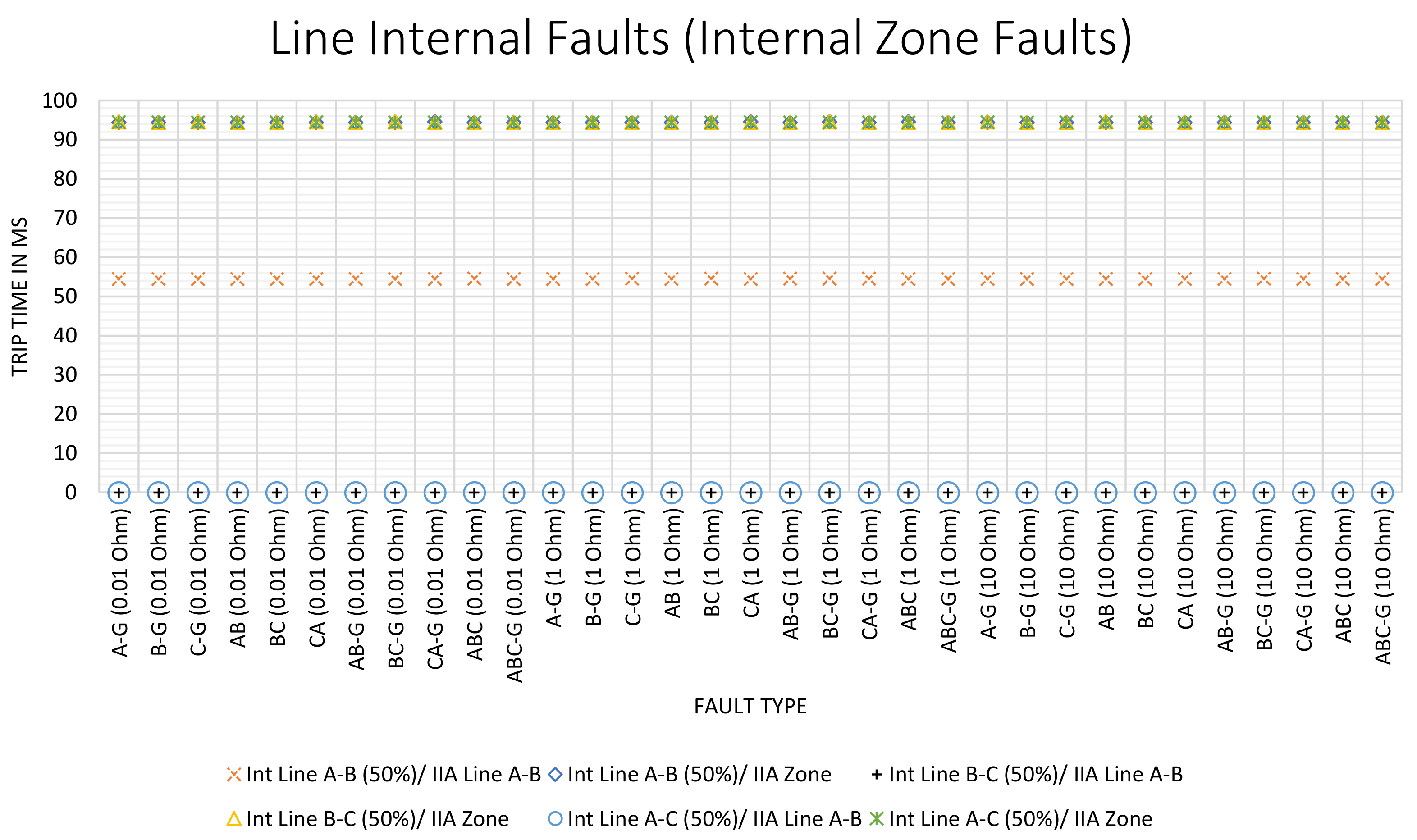
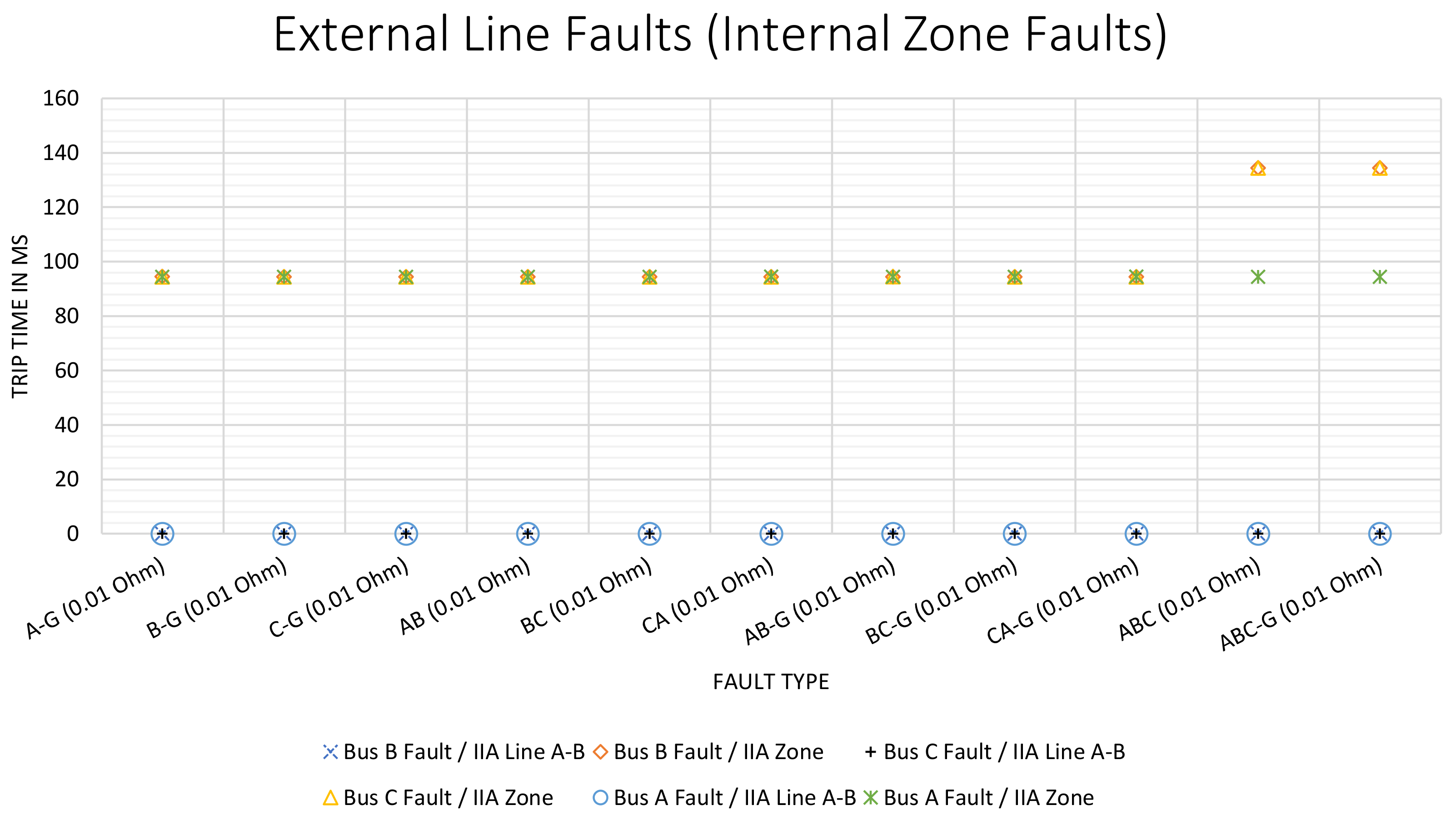
Different fault types and locations were considered. The results of internal line faults (internal zone faults) are represented in Figure 11. External line fault (internal zone fault) results are represented in Figure 12. For each test, the tripping times of “Line A-B” IIA and $II{A}_{Zone}$ protections were measured. In Figure 11 and Figure 12, the symbols marked with zero trip time mean that no trip was executed by that protection.

In Figure 11 it can be observed that all the tripping commands were executed for internal faults in line A-B and internal zone faults. In contrast, no trip for line A-B was executed for faults in lines B-C and A-C (external faults of line A-B), as desired. All the internal faults of the protected zone were detected and cleared. Overall, the average delay of the trip times observed for IIA protection of line A-B is 54.47 ms. The average of the trip times observed for $II{A}_{Zone}$ protection is 94.45 ms. Therefore, the results of the tests are correct.

In Figure 12 it can be observed that no trip commands were executed in the line A-B for faults in Bus A, Bus B and Bus C. As desired, all the internal faults of the protected zone were detected and cleared: in the figure they are presented as the symbols with zero trip time. The average time of the trips observed for the $II{A}_{Zone}$ protection is 99.29 ms. Therefore, the results of the tests are correct.

As a result of the tests performed for the external zone faults (Side A, Side B and Side C), it is observed that no trip commands were executed in line A-B or in the protected zone; this is the desired behaviour.

• 400 kV Transmission system with RES.

In

Table 8. $II{A}_{Zone}$ behaviour with RES (Part 1 of 2).

Fault Type	Internal Zone Fault “Line A-B”	External Zone Fault “Side B”
A-G
AB

and

Table 9. $II{A}_{Zone}$ behaviour with RES (Part 2 of 2).

Fault Type	Internal Zone Fault “Line A-B”	External Zone Fault “Side B”
AB-G
ABC
ABC-G

, the behaviour of the $II{A}_{Zone}$ protection is represented by the signal “Zone_II_Angle” (red colour), and the behaviour of line IIA is represented by the signal “Line_Axions_II_Angle” (blue colour). The signal “Fault_RTDS_FAULT” represents the exact moment when the RTDS generates the fault in the power system, the signal “Line_Axions_TRIP_IIA_AXIONS” represents the trip signal of the line IIA protection method, and the signal “Zone_TRIP_IIA_ZONE” represents the trip signal of the $II{A}_{Zone}$ protection method. In the first column (“Fault Type”), the fault types that have been considered are represented: A-G, AB, AB-G, ABC, and ABC-G. The other fault types have a similar behaviour. The second column represents the behaviour of the protection methods with a fault inside the line A-B (internal zone fault). The third column represents the behaviour of the protection methods with an external zone fault in Side B.

In Table 8 and Table 9, it can be observed that the sign of the IIA applied to a line and the $II{A}_{Zone}$ applied to a zone, in an operating condition without fault, provide a negative value near −90°. When an internal fault occurs, this angle suddenly changes to a positive one greater than 5° and lesser than 90°. This is the correct behaviour.

The trip time obtained in each test with RES on Side B can be observed in Figure 13 and Figure 14. These times were measured by the RTDS as the interval between the generation of the fault by the power system and the moment when the fault is cleared by the corresponding protection method.

Different fault types were executed in different locations. Internal line faults (internal zone faults) results are represented in Figure 13. External line faults (internal zone faults) results are represented in Figure 14. For each test, the tripping times of Line A-B IIA and $II{A}_{Zone}$ protection were measured. As before, the symbols with zero trip time mean that no trip was executed by that protection.

In Figure 13 it can be observed that trip commands were executed for internal faults in line A-B and internal zone faults. No trip for line A-B was executed for faults in lines B-C and A-C (external faults of line A-B). All the internal faults of the protected zone were detected and cleared. In some cases, no trip was executed (the symbols with zero trip time). The average of the trip times observed for IIA protection of line A-B was 53.65 ms, and the average of the trip times observed for $II{A}_{Zone}$ protection was 94.34 ms.

In Figure 14 it can be observed that no trip commands were executed in line A-B for faults in Bus A, Bus B, and Bus C. All internal faults of protected zones were detected and cleared. In Figure 14, symbols marked with zero trip time mean that no trip was executed by that protection. The mean of the trip times observed for $II{A}_{Zone}$ protection is 98.95 ms.

The results obtained from external zone fault (Side A, Side B, and Side C) tests conclude that no trip commands were executed in line A-B or in protected zone. This behaviour is correct.

• Behaviour with different fault resistances.

This subsection studies the behaviour of IIA as a function of fault resistance. The transmission system is studied with and without RES. Fault resistances of 0.01 Ω, 1 Ω, and 10 Ω have been tested. Considering that all fault types have a similar behaviour, only A-G faults have been represented (

Table 10. $II{A}_{Zone}$ behaviour, different fault resistance, with and without RES.

Fault Type	Internal Zone Fault “Line A-B” without RES	Internal Zone Fault “Line A-B” with RES
A-G (0.01 Ω)
A-G (1 Ω)
A-G (10 Ω)

).

In Table 10, the behaviour of the $II{A}_{Zone}$ is represented by the signal “Zone_II_Angle” (red colour), and the behaviour of line IIA is represented by the signal “Line_Axions_II_Angle” (blue colour). The signal “Fault_RTDS_FAULT” represents the exact moment when the RTDS generates the fault in the power system; the signal “Line_Axions_TRIP_IIA_AXIONS” represents the trip signal of the line IIA protection method; and the signal “Zone_TRIP_IIA_ZONE” represents the trip signal of the $II{A}_{Zone}$ protection method.

The second column of the table represents the behaviour of protection methods with a fault inside line A-B (internal zone fault) without RES. The third column represents the behaviour of protection methods with a fault inside line A-B (internal zone fault) with RES.

From the results presented in Table 10, it can be observed that the sign of both the IIA applied to a line and the $II{A}_{Zone}$ applied to a zone, in an operating condition without fault, provide a negative value near −90°. When an internal fault occurs, this angle changes to a positive value greater than 5° and lesser than 90°. This behaviour is correct.

Observing the results, it is seen that when the fault resistance is increased, the integrated impedance angle in fault state gets closer to the 5° limit. Therefore, it can be concluded that the proposed method is sensitive to fault resistance, so an internal fault may be undetected with a fault resistance higher than 10 Ω. Methods for dealing with this problem can be studied in future works.

7. 150 kV Submarine Transmission Grid

The FARCROSS project also considers interconnections with some islands in Greece. Within the project, a short-circuit protection method is being proposed and implemented in 150 kV submarine lines.

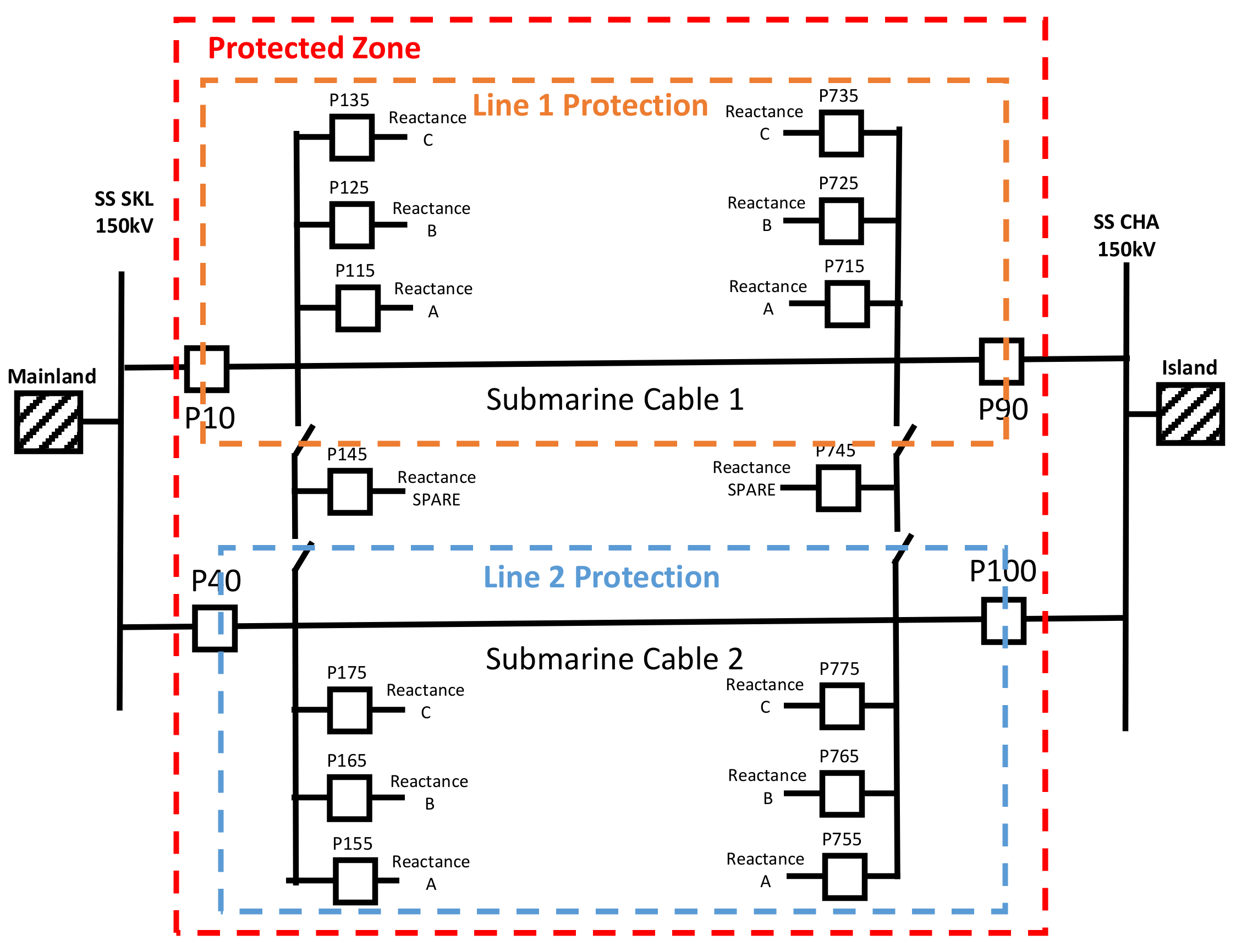
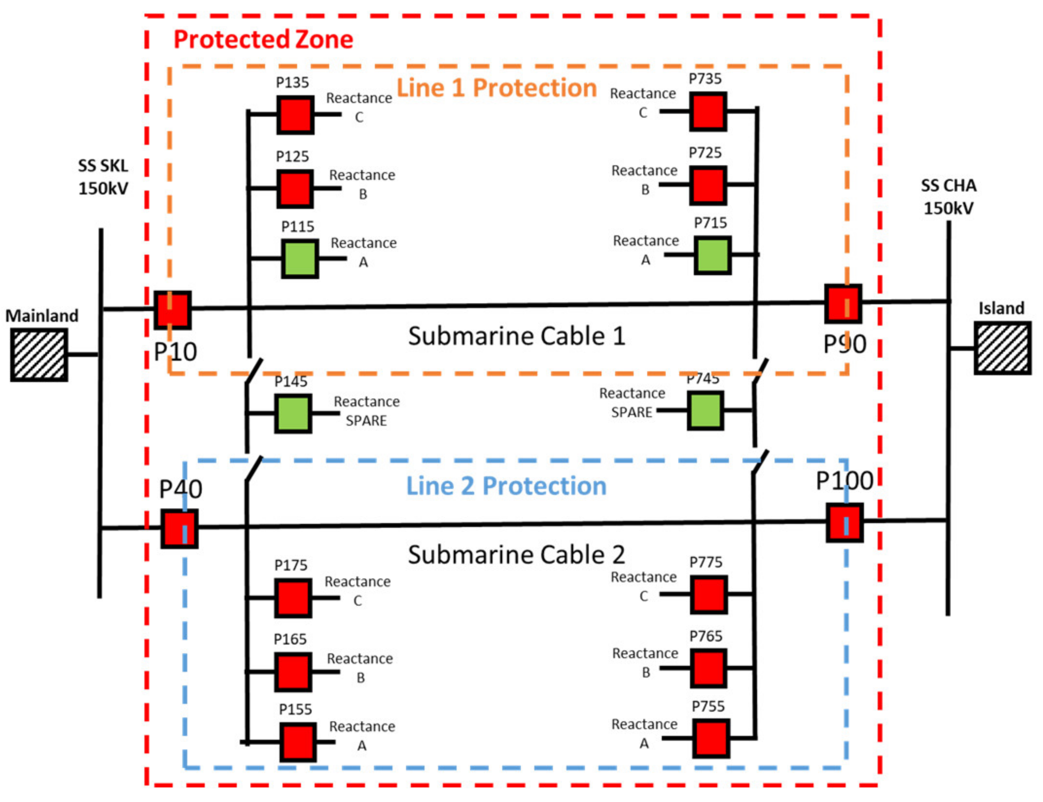
A general one-line diagram of the interconnection lines can be seen in Figure 15. The PMUs will be installed in breakers P10 and P40 of a substation (denoted as “SS SKL” in Figure 15) and in breakers P100 and P90 of another one (denoted as “SS CHA” in Figure 15).

Specifically, the interconnection lines consist of two submarine cables (each 135 km long) making this the longest sub-sea alternating current connection in the world [31], between “SS SKL” and “SS CHA”. The main layout of “SKL” and “CHA” substations is comprised of seven reactors with a capacity of 40 MVAr each and two 150 kV bays of submarine interconnection lines which connect both substations. Four PMUs will be installed in the submarine interconnections lines SKL–CHA. These PMUs receive measurements from current transformers (CT) and potential transformers (PT) which are installed at each bay of the circuit.

The reactors are not always connected to the system and their function depends on the load conditions. Based on the TSO’s plan and the current load conditions, all the reactors may be connected (except AYT-4, which is disconnected). Nevertheless, if the loading conditions change, then it is possible that their operation is likely to change as well.

The implementation in the RTAC is aimed at protecting each line independently with the IIA method, and as a backup, to protect the zone with the $II{A}_{Zone}$ protection method. The protection zones implemented in the submarine interconnections between “SS SKL” and “SS CHA” can be observed in Figure 16.

For this setup, the time delay to trip for the IIA line protections is set to 40 ms and for $II{A}_{Zone}$ protection is set to 200 ms. The main objective of this setting is to guarantee a good time coordination and selectivity between zones.

To evaluate the behaviour of the proposed method in a submarine transmission grid, the following scenario was implemented (see Figure 17).

The electrical data of generators, transmission lines, Submarine Cable 1, Submarine Cable 2, and reactors can be found in

Table 11. Generators’ data for submarine transmission system.

Generator Data	Side A	Side B	Side C
Nominal Voltage (kV)	150	150	150
Phase (deg)	−10	15	20
Frequency (Hz)	50	50	50
Inductance Series + (Henry)	0.1	0.1	0.1
Resistance Series + (Ohm)	3.14	3.14	3.14
Inductance 0 Parallel (Henry)	0.1	0.1	0.1
Resistance 0 Parallel (Ohm)	3.14	3.14	3.14

,

Table 12. 150 kV Transmission lines’ Data.

Line BC and Line CA
Model	Bergeron (RLC)
Line Length (km)	100
Positive Sequence Series Resistance (Ohm/km)	0.0293
Positive Sequence Series Ind. Reactance (Ohm/km)	0.3087
Positive Sequence shunt Cap. Reactance (MOhm·km)	0.2664
Zero Sequence Series Resistance (Ohm/km)	0.3
Zero Sequence Series Ind. Reactance (Ohm/km)	0.988
Zero Sequence Shunt Cap. Reactance (MOhm·km)	0.4369

,

Table 13. Data of Submarine Cable 1.

Submarine Cable 1
Model	Bergeron (RLC)
Line Length (km)	179
Positive Sequence Series Resistance (Ohm/km)	0.057825
Positive Sequence Series Ind. Reactance (Ohm/km)	0.11565
Positive Sequence shunt Cap. Reactance (MOhm·km)	0.0167531519
Zero Sequence Series Resistance (Ohm/km)	0.414648
Zero Sequence Series Ind. Reactance (Ohm/km)	0.1928601
Zero Sequence Shunt Cap. Reactance (MOhm·km)	0.0167531519

,

Table 14. Data of Submarine Cable 2.

Submarine Cable 2
Model	Bergeron (RLC)
Line Length (km)	179
Positive Sequence Series Resistance (Ohm/km)	0.043425
Positive Sequence Series Ind. Reactance (Ohm/km)	0.118575
Positive Sequence shunt Cap. Reactance (MOhm·km)	0.0163235839
Zero Sequence Series Resistance (Ohm/km)	0.233361
Zero Sequence Series Ind. Reactance (Ohm/km)	0.1099303
Zero Sequence Shunt Cap. Reactance (MOhm·km)	0.0163235839

, and

Table 15. Data of reactors.

Reactors
Rated Voltage (kV)	150
Reactive Power (MVAr)	40
Inductance (Henry)	1.79049310978

, respectively.

To evaluate the behaviour of the proposed method, different kinds of faults were executed in different locations of the 150 kV transmission system, as we will next see.

7.1. Tests Executed in the 150 kV Submarine Transmission Grid

This section describes the tests performed to evaluate the behaviour of the proposed method. Two scenarios of reactive compensation in Submarine Cable 1 were considered during the tests:

(a)

Scenario 1: Four reactors are connected (see Figure 18).

(b)

Scenario 2: Two reactors are connected (see Figure 19).

In Figure 18 and Figure 19, the breakers in red colour are closed and those in green colour are opened. The following set of fault locations is proposed for each scenario (see Figure 20).

For internal line faults different types of faults are proposed: A-G, B-G, C-G, AB, BC, CA, AB-G, BC-G, CA-G, ABC, and ABC-G, with different fault resistances. When a fault exists in a submarine cable, the fault resistances are supposed to be very low, because the rupture of dielectric isolation caused by degradation may occur quickly. Assuming that the worst scenario in fault resistance may be a fault in an overhead section of the line near the substations, and taking as a reference the fault resistances estimated in studies [29,30], in this study we use the fault resistance values of 0.01 Ω, 1 Ω, and 10 Ω.

For external line/zone faults, different types of faults are proposed: A-G, B-G, C-G, AB, BC, CA, AB-G, BC-G, CA-G, ABC, and ABC-G, with a fault resistance of 0.01 Ω.

For each test it is necessary to evaluate the behaviour of all protections. No fault detection is expected for external faults, but only for internal faults, to guarantee the selectivity of the proposed method.

During these tests, the process cycle rate used in the RTAC to implement the proposed algorithm is one cycle per 1 ms (10 ms was the value used in Section 6). This parameter is changed to further reduce the response time of the protection; 1 ms is the highest frequency supported by the RTAC. The PMUs data is updated every 10 ms.

The expected time delay to trip for lines IIA protection is 40 ms after pickup of the function. The expected time delay to trip for Zone IIA protection is 200 ms after pickup of the function. The duration of each fault is 1 s, in order to have enough time to observe the behaviour of the protection algorithms.

Overall, 330 different tests have been executed in the 150 kV transmission system, as we will see next.

7.2. Results Obtained in the 150 kV Submarine Transmission Grid with Four Reactors Connected

• Internal Fault in Line 1: Four reactors connected.

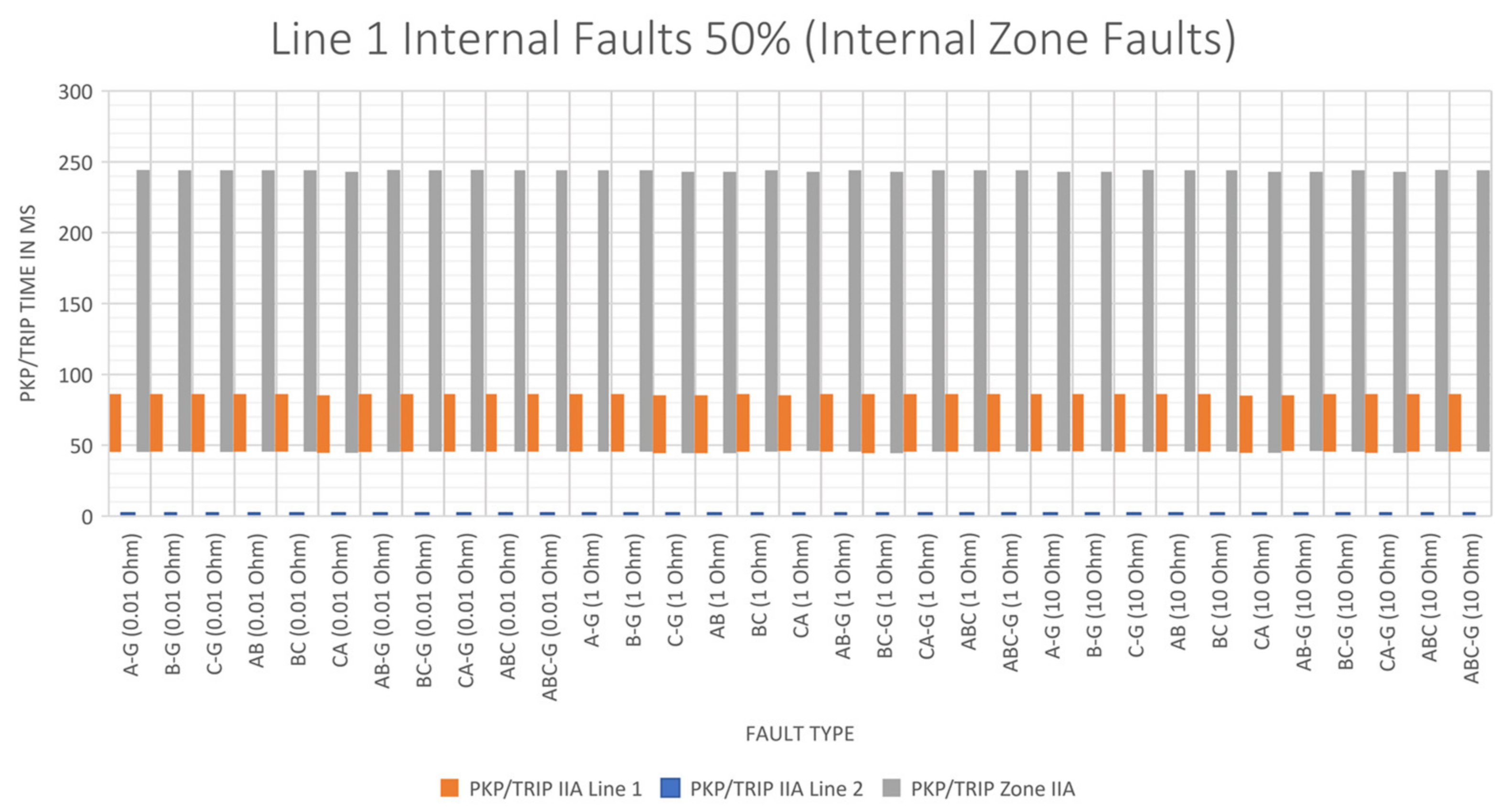
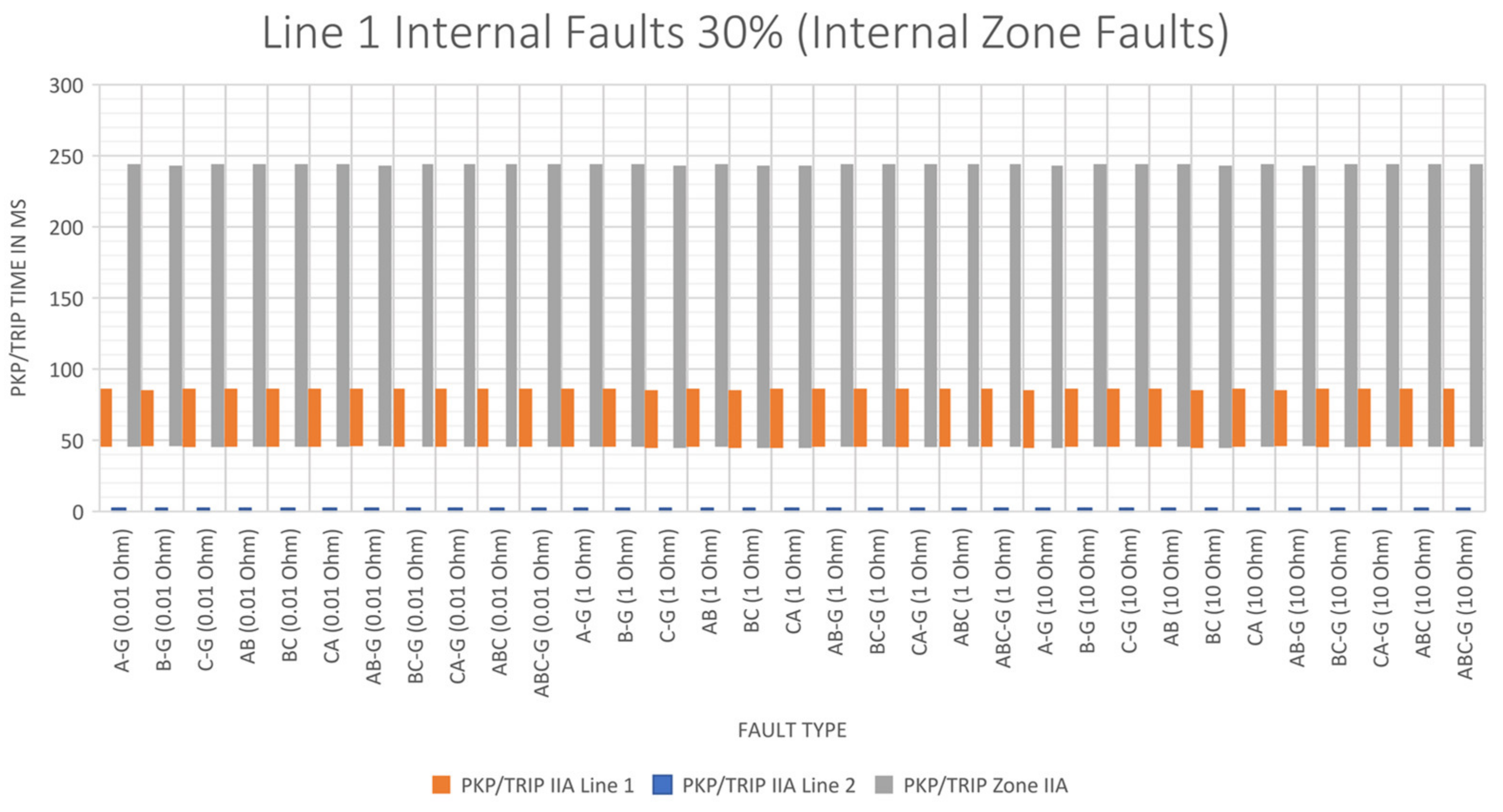
In Figure 21, the test results for internal faults at 50% of Line 1 (just in the middle), with a fault resistance of 0.01 Ω, 1 Ω, and 10 Ω, can be observed. Figure 22 presents the same results if the fault is at 30% of the same line, and Figure 23 shows the results for internal faults at 70% of the line.

The bars in these figures represent the time between the pickup time and the trip time for IIA protection of Line 1 (orange bar), IIA protection for Line 2 (blue bar), and $II{A}_{Zone}$ protection (grey bar). Each bar starts at the pickup time. A bar near 0 ms represents that no pickup nor trip was detected by that specific protection.

From the results observed in Figure 21, Figure 22 and Figure 23, it can be concluded that all the faults were detected by IIA Line protection in Line 1, no internal fault was detected by IIA Line protection in Line 2, and all faults were detected by $II{A}_{Zone}$ protection.

In IIA Line protection of Line 1, the maximum pickup time obtained was 45.76 ms, the minimum one was 44.32 ms, with an average of 45.15 ms. The average of the trip times was 40.93 ms (40 ms was the expected value).

In $II{A}_{Zone}$ protection, the maximum pickup time obtained was 45.76 ms, whereas the minimum was 44.32 ms, with an average of 45.15 ms. The average of the trip times obtained after pickup was 198.77 ms (200 ms was the expected value). Therefore, these results are correct, considering this acceptable tolerance.

• Internal Fault in Line 2: Four reactors connected.

In Figure 24 the test results for internal faults can be observed at 50% of Line 2, with a fault resistance of 0.01 Ω, 1 Ω, and 10 Ω. The colors are the same as the ones used in the previous subsection.

From the results shown in Figure 24, it can be concluded that all the faults were detected by IIA line protection in Line 2, no internal fault was detected by IIA Line protection in Line 1, and all faults were detected by $II{A}_{Zone}$ protection, which is the desired behaviour.

In IIA Line protection of Line 2, the maximum pickup time obtained was 45.6 ms, and the minimum one was 45.12 ms, with an average of 45.29 ms. The average trip time after pickup was 40.91 ms (40 ms was the expected value).

In $II{A}_{Zone}$ protection, the maximum pickup time obtained was 45.6 ms, the minimum was 45.12 ms, with an average of 45.29 ms. The average trip time after pickup was 198.91 ms (200 ms was the expected value). Therefore, these results are correct, considering this acceptable tolerance.

• External Zone Fault: Four reactors connected.

The test run for external Lines/Zone faults in Side A, Side B, and Side C, with a fault resistance of 0.01 Ω showed that, for external line/zone faults, no trip was executed by IIA Line protection in Line 1, IIA Line protection in Line 2, and $II{A}_{Zone}$ protection, as expected.

Some Pickup–Dropouts were detected in the tests: pulses lasting between 18.72 and 21.76 ms for IIA Line protection and pulses with a duration between 17.76 and 42.4 ms for $II{A}_{Zone}$ protection, but no trip did appear.

7.3. Results Obtained in 150 kV Submarine Transmission Grid with Two Reactors Connected

• Internal Fault in Line 1: Two reactors connected.

In Figure 25, the test results for internal faults at 50 % of Line 1 with a fault resistance of 0.01 Ω, 1 Ω, and 10 Ω are presented. Figure 26 presents the test results for internal faults at 30% of the same line, and Figure 27 the test results for internal faults at 70% of the line.

Test results presented in Figure 25, Figure 26 and Figure 27 show that all faults were detected by IIA Line protection in Line 1, no internal fault was detected by IIA Line protection in Line 2, and all faults were detected by IIA zone protection.

In IIA Line protection of Line 1, the maximum pickup time obtained was 65.76 ms, the minimum was 44.32 ms, and the average was 48.06 s. The average trip time obtained after pickup was 40.95 ms, with 40 ms being the expected value.

In $II{A}_{Zone}$ protection, the maximum pickup time obtained was 65.76 ms, the minimum time was 44.32 ms, and the average was 48.07 ms. The average trip time obtained after pickup was 199.19 ms (200 ms was the expected value).

• Internal Fault in Line 2: Two reactors connected.

In Figure 28 can be observed the test results for internal faults at 50% of the Line 2 with a fault resistance of 0.01 Ω, 1 Ω, and 10 Ω.

Test results presented in Figure 28 show that all the faults were detected by IIA Line protection in Line 2, no internal fault was detected by IIA Line protection in Line 1, and all the faults were detected by $II{A}_{Zone}$ protection.

In IIA Line protection of Line 2, the maximum pickup time obtained was 46.72 ms, the minimum was 44.48 ms, and the average was 45.38 ms. The average trip time obtained after pickup was 40.79 ms. The expected value was 40 ms.

In $II{A}_{Zone}$ protection, the maximum pickup time obtained was 65.44 ms, the minimum was 44.48 ms, and the average was 46.59 ms. The average trip time obtained after pickup was 199.27 ms (200 ms was the expected value).

• External Zone Fault: Two reactors connected.

Test results for external line/zone faults in Side A, Side B, and Side C, with a fault resistance of 0.01 Ω showed that, for external line/zone faults, no trip was executed by IIA Line protection in Line 1, IIA Line protection in Line 2, and $II{A}_{Zone}$ protection, as expected.

Some pickup–dropouts were detected. Pulses with a duration between 19.84 and 21.28 ms for IIA Line protection of Line 2 and pulses between 19.84 and 21.28 ms for $II{A}_{Zone}$ protection were observed. With these results, it is concluded that the algorithm is behaving as expected.

7.4. Test Summary: 150 kV Submarine Transmission Grid

The pickup time of the proposed protection method is between 44.32 and 66.88 ms. The obtained average time is 48.52 ms considering all the executed tests that resulted in a trip.

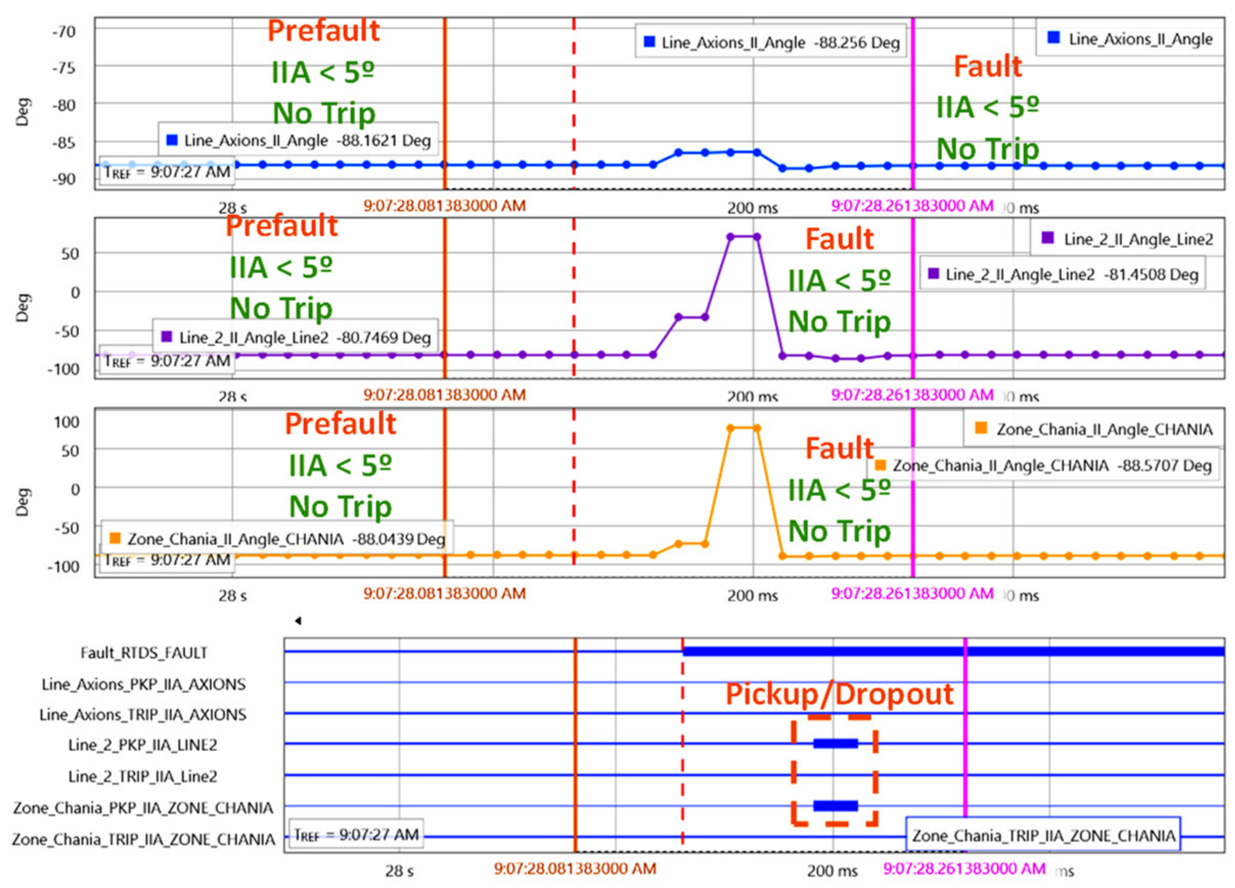
In Figure 29 the typical behaviour of IIA Line/$II{A}_{Zone}$ protections for an internal fault in Line 1 can be observed. Note that Line 2 continues viewing an external fault, because its IIA is always under 5°. When the IIA in fault state of Line 1 and Zone crosses the limit of 5°, it reaches 28.15° and 26.82°, respectively. In this condition, the trips are executed after the expected time delay.

Figure 30 shows the typical IIA behaviour with an internal fault in Line 2. Note that Line 1 continues viewing an external fault because its IIA is always under 5°. When the IIA in fault state of Line 2 and Zone crosses the limit of 5°, it reaches 53.51° and 35.14°, respectively. In this condition, the trips are executed after the expected time delay.

Figure 31 presents the typical IIA behaviour with an external line/zone fault. Note that Line 1, Line 2, and Zone continue viewing an external fault because their IIA is always under 5°. In some tests, a transient is detected, generating a pickup and dropout pulse of the function. This pulse lasts between 18.72 and 21.76 ms for IIA Line protection, and between 17.76 and 42.4 ms for $II{A}_{Zone}$ protection. With this finding, it is set clear that the time delay for the trip of Line IIA protection cannot be set under 30 ms, and the time delay for trip setting for $II{A}_{Zone}$ protection cannot be set under 50 ms. This setting limit permits one to avoid undesired trips for external line/zone faults.

All in all, 330 tests have been executed using this power system. In all of them, a good behaviour of the $II{A}_{Zone}$ protection method was observed. Furthermore, internal zone faults were detected, and trips were generated, and in the presence of external zone faults, the method is stable and did not generate any undesired trips. With these test results, it is concluded that Line IIA and $II{A}_{Zone}$ protection methods work correctly as backup protections for the 150 kV Line 1 and 150 kV Line 2 between “SS SKL” and “SS CHA”.

8. Discussion

The sign of the IIA applied to a line and the $II{A}_{Zone}$ applied in a zone to be protected, in an operating condition without fault, has a negative value near −90°. When an internal fault occurs, this angle changes to a positive one greater than 5° and lesser than 90°. This behaviour is consistent with the operating characteristics of the $II{A}_{Zone}$ protection scheme represented in Figure 5, and has been observed during the tests performed with the algorithm.

Observing these results, when the fault resistance increases, the integrated impedance angle in fault state approximates to the 5° limit. The efficiency of the proposed method for higher fault resistance values may be evaluated in future studies.

For external faults, the proposed algorithm is stable and secure in its operation. Not a single trip was executed for external faults and no trip was executed in no-fault condition, with and without RES.

The protection algorithm can be easily time-coordinated with traditional protection relays such as distance protection (21), line differential relays (87L), and overcurrent relays (50/51), considering the pickup times observed during the tests (between 44 and 65 ms). By the configuration of an appropriate time delay, time coordination with other protection elements or functions in the network can be achieved.

During the 400 kV transmission tests (Section 6), the average trip time obtained in the executed tests for $II{A}_{Zone}$ protection method was 94.45 ms without RES and 94.08 ms with RES. The average trip time obtained in the IIA method applied to Line A-B is 54.47 ms without RES and 53.65 ms with RES. During these tests, the process rate used in the RTAC to implement the proposed algorithm was one cycle per 10 ms, considering that PMUs data was updated every 10 ms.

As far as 150 kV transmission tests are concerned (Section 7), the average pickup time obtained for IIA Line protection and $II{A}_{Zone}$ protection was 48.52 ms, considering all the tests that resulted in a trip. The obtained average trip times after pickup for IIA Line protection was 40.95 ms. This can be considered a good result, since the programmed value was 40 ms. Regarding Zone IIA protection, the delay was 199 ms (200 ms was the expected one).

Comparing both 150 and 400 kV transmission tests, a reduction in the pickup time in the order of 45 ms can be observed (94.45 vs. 48.52 ms) for $II{A}_{Zone}$ protection, and a reduction of 6 ms (54.47 vs. 48.52 ms) for IIA Line protection.

Considering the trip times observed during the tests, it is set clear that these algorithms are well suited to implement backup protections in transmission grids, given that backup trip times in transmission grids are usually set between 400 and 1000 ms. The actuation times obtained by the proposed algorithms in the tests support their capability of being used as backup protections even in scenarios with penetration of renewable energies.

9. Conclusions

This article has presented a new wide-area backup protection method as an alternative to Zone 3 protection method or traditional protection backup schemes. The proposed method ($II{A}_{Zone}$) merges the theory of IIA [14,15] for line protection and the theory of virtual buses [16,19] to define a protected zone.

The proposed method uses the time-synchronized positive sequence phasors of voltages and currents supplied by PMUs based in Std. IEEE C37.118 of all inputs’ and outputs’ location of the protected zone, being easy to parametrize and to implement in real power systems, due to its simplicity and its low number of settings.

The behaviour of the proposed method in the presence of internal and external faults in the protection zone has been tested using a real time laboratory with commodity PMUs and an RTDS simulator. The proposed method has been tested with three different fault resistance values. A total number of 990 tests in two scenarios have been run: a 400 kV, with (330 tests) and without (330 tests) RES and a 150 kV submarine transmission system (330 tests).

The trip times observed during the tests (always below 100 ms) show that the algorithm has a good behaviour so it can be used as a backup protection scheme, considering that traditional protection schemes have a trip time in order of 400–1000 ms. The behaviour of the proposed method is stable, reliable, obedient, and secure, also with RES installed in the power system. In addition, the method is selective, i.e., no trip was executed for external faults, no trip was executed in no-fault condition, and all internal faults applied were detected and tripped correctly. Finally, the results show that the method is sensitive to fault resistance, so an internal fault may be undetected with a fault resistance bigger than 10 Ω. Methods for dealing with this problem can be studied in future works.

The protection algorithm can easily be time-coordinated with traditional protection relays such as distance protection (21), line differential relays (87L), and overcurrent relays (50/51) considering the pickup times observed during testing (between 44 and 65 ms) and configuring an appropriate time delay for trip to guarantee the coordination time.

This method can be applied to a wide area and multiple zones as a backup protection in transmission systems in order to avoid unnecessary Zone 3 tripping on load encroachment during wide area disturbances that may result in quick deterioration of the system and possible partial blackouts.

As future work, the algorithm will be tested in the field using the PMUs that are being deployed in different Greek substations within the H2020 FARCROSS project. These tests will provide good insight about the behaviour of the algorithm in a real environment. In addition, the behaviour of the algorithm in bigger scenarios could be tested.