Article

Evaluation of Various Tree-Based Ensemble Models for Estimating Solar Energy Resource Potential in Different Climatic Zones of China

1
Shenzhen Longhua High School, Longhua District, Shenzhen 518109, China
2
School of Resource and Environmental Science, Wuhan University, Wuhan 430079, China
3
College of Public Administration, Huazhong Agricultural University, Wuhan 430070, China
4
Laboratory of Critical Zone Evolution, School of Earth Sciences, China University of Geosciences, Wuhan 430074, China
*
Author to whom correspondence should be addressed.
Energies 2022, 15(9), 3463; https://doi.org/10.3390/en15093463
Submission received: 24 March 2022 / Revised: 3 May 2022 / Accepted: 5 May 2022 / Published: 9 May 2022

Abstract

:
Solar photovoltaic (PV) electricity generation is growing rapidly in China. Accurate estimation of solar energy resource potential (Rs) is crucial for siting, designing, evaluating and optimizing PV systems. Seven types of tree-based ensemble models, including classification and regression trees (CART), extremely randomized trees (ET), random forest (RF), gradient boosting decision tree (GBDT), extreme gradient boosting (XGBoost), gradient boosting with categorical features support (CatBoost) and light gradient boosting method (LightGBM), as well as the multi-layer perceotron (MLP) and support vector machine (SVM), were applied to estimate Rs using a k-fold cross-validation method. The three newly developed models (CatBoost, LighGBM, XGBoost) and GBDT model generally outperformed the other five models with satisfactory accuracy (R2 ranging from 0.893–0.916, RMSE ranging from 1.943–2.195 MJm−2d−1, and MAE ranging from 1.457–1.646 MJm−2d−1 on average) and provided acceptable model stability (increasing the percentage in testing RMSE over training RMSE from 8.3% to 31.9%) under seven input combinations. In addition, the CatBoost (12.3 s), LightGBM (13.9 s), XGBoost (20.5 s) and GBDT (16.8 s) exhibited satisfactory computational efficiency compared with the MLP (132.1 s) and SVM (256.8 s). Comprehensively considering the model accuracy, stability and computational time, the newly developed tree-based models (CatBoost, LighGBM, XGBoost) and commonly used GBDT model were recommended for modeling Rs in contrasting climates of China and possibly similar climatic zones elsewhere around the world. This study evaluated three newly developed tree-based ensemble models of estimating Rs in various climates of China, from model accuracy, model stability and computational efficiency, which provides a new look at indicators of evaluating machine learning methods.

1. Introduction

Achieving a clear and accurate understanding of global solar radiation/solar energy resource potential (Rs) is critical to the assessment and design of solar energy development and utilization [1]. Over the past two decades, solar photovoltaic (PV) installation capacity in China has rocketed from less than 1 GW in 2000 to 175 GW in 2018, ranking first in the world [2]. To achieve its “Carbon Neutrality” pledge to the United Nations, the Chinese government has set a series of goals regarding developing renewable energy, one of which is that PV maximal installation capacity is expected to reach 2000 GW by 2050 [3]. Therefore, accurate determination and clear understanding of Rs is crucial for siting, evaluating and optimizing solar energy systems. Unfortunately, the stations observing Rs are very sparse around the world due to high instrument costs and technical requirements [4], particularly for developing countries such as China [5]. Therefore, developing and employing different algorithm techniques to predict Rs has been a heavily researched topic in recent years. In general, there are three different model types to estimate Rs: the empirical models, physical transmission models and machine learning models.

1.1. A Review of Empirical Models for Rs Estimation

Various types of empirical models have been established for Rs estimation from single or hybrid-measured meteorological parameters, such as temperature-based models [6], cloud-based models [7], sunshine-based models [8], day of the year-based models [9] and hybrid variables-based models [10]. For example, Fan et al. [6] proposed six new temperature-based models to estimate daily Rs in the south of China, and the results indicated that the newly proposed models exhibited better accuracy than existing temperature-based empirical models. Fan et al. [8] also proposed and compared various sunshine-based models for modeling Rs at 20 sites in China. It was found that the values of R2 and RMSE for the best model were lower than 0.9 and more than 2.4 MJ m−2day−1, respectively. Zang et al. [9] applied various day of the year-based models for modeling Rs at 35 stations in various climatic zones of China and found that the newly proposed model obtained the best performance. Chen et al. [11] conducted a comprehensive study to review and apply 294 different types of empirical models in China. However, the amount of Rs reaching the surface is greatly affected by geographical, meteorological and terrestrial factors, and the abovementioned empirical models do not explain the mechanisms, atmospheric transmittance process and the need to be re-calibrated from one site to another [12]. Thus, it is limited in general applicability in remote regions and inconvenient for calibrated parameters.

1.2. A Review of Physical Transmission Models for Rs Estimation

The physical transmission models take into consideration the physical process, which provides alternative ways to predict Rs: for example, Gueymard [13,14] proposed a physically based model for estimating the diffuse and clear-sky beam. Yang et al. [15] and Yang et al. [16] developed a hybrid model to estimate the hourly, daily, and monthly Rs. Qin et al. [17] also developed an efficient physically based parameterization radiation model to estimate Rs in different sky conditions. Sun et al. [18] and Sun and Liu [19] proposed a fast scheme called SUNFLUX for estimating Rs based on the full radiation scheme, and the results showed that the accuracy of SUNFLUX for 30-minite data was in good agreement with observations. Tang et al. [20] employed the fast parameterization scheme to estimate instantaneous and daily Rs based on MODIS products, and the R2 and RRMSE values for daily Rs were 0.92 and about 16%, respectively. However, previous studies have shown that their accuracy need to be further improved compared to machine learning models. For instance, Chen et al. [4] compared the accuracy of different machine learning models and Yang’s hybrid model and found that the latter performed worst among all models. Qin et al. [21] applied eight artificial intelligence (AI) models and four physically based models to estimate daily photosynthetically active radiation (PAR) in China; the results showed that the four physically based models performed worse than the eight AI models. Moreover, these physical transmission models often simulate interaction between Rs and the atmosphere, and this simulation requires many input variables (e.g., moisture, surface albedo, and aerosol optical depth) that are difficult to obtain. It is apparent from the calculating process that the model performances depended on input meteorological variables.

1.3. A Review of Artificial Neural Network (ANN) Models for Rs Estimation

In recent years, various machine learning models, as particularly promising approaches, have been proposed and widely employed for estimating Rs [22]. Artificial neural network (ANN) models have been successfully applied in estimating Rs. For example, Wang et al. [12] compared and evaluated an empirical model and three types (MLP, GRNN and RBNN) of ANN algorithms for modeling Rs in China, and it was found that RBNN and MLP algorithms performed slightly superior to the empirical models and GRNN. Kaba et al. [23] developed a new DLNN model for predicting Rs and found that the model performed well, with R2 and RMSE of 0.98 and 0.78 MJm−2d−1, respectively. Sun et al. [24] estimated Rs from two datasets by training the video image using the CNN model, and obtained fair NRMSE values of 26–30%. Vakili et al. [25] estimated daily Rs in Tehran, Iran using ANN and MLP models, and the result showed R2, RMSE and MAPE to be 0.99, 0.05 J cm−2d−1 and 1.5%, respectively.
The hybrids of ANN models with other modeling techniques have also been studied worldwide to improve the prediction accuracy of modeling Rs [26]. For example, Qin et al. [21] applied a BP neural network coupling mind evolutionary model to predict photosynthetically active radiation (PAR) and found that the hybrid model performed best among all 12 models and the R, RMSE and MAE for the optimized model were 0.986, 0.393 MJ m−2day−1 and 0.302 MJ m−2day−1, respectively. Heng et al. [27] developed a hybrid model on the basis of four ANN models to estimate Rs at six sites in America, and the results showed that the proposed hybrid model performed better in terms of stability and prediction accuracy. Mousavi et al. [28] estimated daily Rs in Mashhad, Iran using a hybrid model combining simulated annealing (SA) and ANN, called ANN/SA, and the results showed that the ANN/SA model performed superior to the single ANN or SVM model. Deo et al. [29] adopted a support vector machine coupling wavelet (W-SVM) model to predict Rs, and found that the developed model performed well, with MAPE, RRMSE and R values ranging 4.696–6.20%, 5.942–7.66% and 0.958–0.965, respectively, in Italy. Wang et al. [30] applied ANFIS with subtractive clustering (ANFIS-SC), M5Tree, and ANFIS with grid partition (ANFIS-GP) models for modeling daily PAR and found that the two optimized ANFIS models outperformed the empirical methods and the M5Tree model.

1.4. A Review of Tree-Based Ensemble Models for Rs Estimation

Most of the abovementioned artificial intelligence models are relatively complex and require long computational times during the training stage. Meanwhile, few studies evaluated the performances of the models, comprehensively considering computational costs and prediction accuracy. Over the past few years, the common tree-based ensemble models, for example, GBDT, RF, M5Tree and ET models, have been widely applied in estimating Rs [31], because they have good performance for modeling and predicting various time series [32]. For instance, Chen et al. [4] applied five machine learning models (M5Tree, GRNN, BP, MARS and GA) and a physically based model to estimate daily direct horizontal irradiance (DHI) at 16 stations in China, and the result showed that the M5tree was superior to GRNN, YHM, Genetic, BP and MARS models, with the mean RMSE value being 1.989 MJm−2day−1. Fan et al. [33] evaluated the performances of 12 sunshine duration-based models and 12 artificial intelligence models (including M5Tree, RF and GBDT) to estimate daily Rs, and found that the above tree-based models were prospective models for estimating daily Rs. Yagli et al. [34] tested 68 artificial intelligence algorithms for estimating hourly Rs at seven locations in five climatic zones of the United States and found that tree-based models outperformed the other models under all-sky conditions. Voyant et al. [35] applied four regression tree models (normal, pruned, boosted and bagged) to predict intervals for Rs and obtained good prediction bands with a mean interval length (MIL) close to 113 Whm−2 and gamma index lower than 0.9. Yang et al. [36] employed the GBDT model to retrieve daily Rs at a spatial resolution of 5 km from AVHRR, and the results showed the RMSE and R2 values for clear sky conditions were 27.71 Wm−2 and 0.82, respectively, and the values for cloud sky conditions were 42.97 Wm−2 and 0.64, respectively, in China. Jumin et al. [37] applied a boosted decision tree regression (BDRT) model and other conventional regression algorithms, such as a neural network, to predict the changes in solar radiation in Malaysia, and found that BDRT outperformed other models with a high prediction accuracy. Therefore, tree-based models are powerful for regression problems and have the ability to obtain good performance in modeling Rs.
It should be noted that existing studies have shown that the above tree-based methods, such as RF, may encounter an over-fitting problem, i.e., the phenomenon where the model performs well on the training data but poorly on the testing data [38]. Some models may be costly in computational time, i.e., the computational process of models will run inefficiently. Recently, a newly developed tree-based ensemble model, namely, extreme gradient boosting (XGBoost), proposed by Chen and Guestrin [39], has been widely applied in many other fields [40], because it showed better stability and a higher computational efficiency with satisfactory accuracy. For example, Fan et al. [41] applied various artificial intelligence algorithms (including XGBoost and GBDT) to predict daily reference evapotranspiration (ETo), and it was found that the XGBoost and GBDT algorithms showed higher computational efficiency and acceptable stability and accuracy compared to the other four models (SVM, ELM, RF and M5tree).
The other two newly developed tree-based ensemble models, i.e., light gradient boosting method (LightGBM) [42] and gradient boosting with categorical feature support (CatBoost) [43], have been proposed and widely applied in many other fields in the past two years [44]. However, similarly to XGBoost, the two models have also been rarely applied in Rs studies. As far as we know, only Wu et al. [38] tested Catboost’s applicability in daily Rs estimation at only four sites in the south of China. There are no studies focusing on accessing the performances of CatBoost’s applicability for Rs prediction in different climates in China. Meanwhile, the LightGBM model has not yet been applied in modeling Rs around the world despite being widely employed in many other fields.
It can be seen from the above literature reviews that the XGBoost, CatBoost and LightGBM algorithms have not yet attracted much attention in modeling Rs. In addition, comparison of the newly developed tree-based ensemble models (XGBoost, CatBoost and LightGBM) with the common CART, ET, RF, GBDT, MLP and SVM models has not yet been comprehensively performed. Moreover, high computational efficiency and good stability were also essential statistical indicators to consider when applying machine learning techniques, although improving model accuracy is the priority. Therefore, the objectives of this study are to compare the performances (stability, computational time and prediction accuracy) of the three newly developed models with six common models for predicting Rs under various input combinations in contrasting climates.

2. Materials and Methods
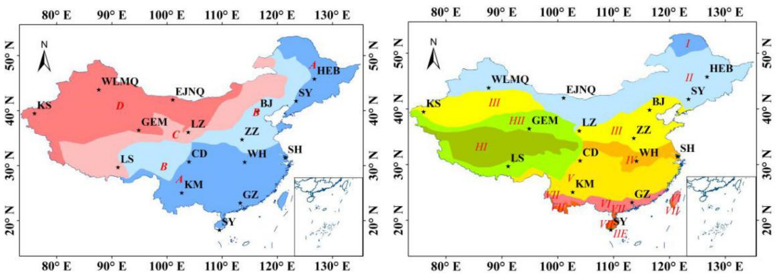
2.1. Study Area

China can be divided into contrasting climatic zones based on precipitation and temperature in this study (Figure 1). There are various characteristics in various climatic zones; for instance, Sanya (SY) station is located at a mid-tropical zone, and the annual mean relative humidity and Tm (80.6% and 25.8 °C, respectively) are the highest among 16 stations in China. Wuhan (WH) is characterized by a north subtropical zone, and the average temperature in January and July are 3 °C and 29.3 °C, respectively. Shenyang (SY) is characterized by a mid-temperate zone with a humid climate; the annual mean rainfall is about 678.8 mm, and the coldest month is January (−11.2 °C), whereas the hottest month is July (25.1 °C).
Existing studies have shown that observed Rs over China may have a large inhomogeneity in decadal variation due to measurement methods, instrument replacement and sensitivity drift before 1993 [45]. Moreover, there were only 17 first-class radiation stations left after 1990. Therefore, only 16 first-class radiation stations (all first-class radiation stations except Mohe station) from 1993–2016 are chosen in this study considering data quality and completeness. The geographical distributions of 16 selected radiation stations in China are shown in Figure 1. As shown in Figure 1, these radiation stations are homogeneously distributed in different climatic zones.

2.2. Data Collection and Quality Control

Daily observed sunshine duration (n), global solar radiation/solar energy resource potential (Rs), relative humidity (Hr), maximum and minimum temperature (Tmax/Tmin), precipitation (Pre), wind speed at 10 m height (U10) and pressure (Prs) during 1993–2016 were collected from 16 stations in different climatic zones of China (Figure 1). Detailed information from 16 meteorological stations is shown in Table 1. To further provide information about the measurements, it can be seen in Table 2 that the sensor types are pyrheliometer and pyranometer in different periods, respectively, and the sampling frequency of the instruments after 1990 are 60 or 360 per hour, respectively. Moreover, the general-purpose lacquer coating on the pyranometers installed in China tended to peel off during the 1980s, and the general-purpose glass did not cover the full solar spectral range and had a lower transmittance than the quart glass, which may degrade instrument sensitivities and lead to a larger negative bias. Therefore, we deleted the dataset of Rs before 1993. The meteorological data were provided by CMA (http://data.cma.cn/, accessed on 1 October 2020). Moreover, extra-terrestrial solar radiation (Ra) and maximum possible sunshine duration (N) were obtained using four equations in Appendix A.
To ensure the daily radiation data quality, the daily radiation data were controlled by the following principles [47]. (1) The observed daily radiation values should not be more than the extra-terrestrial solar radiation values (Ra, MJm−2d−1), i.e., RsRa; despite the fact that global solar radiation could exceed the extra-terrestrial solar radiation value due to the enhancement effect of clouds, it’s usually limited in the case of the minute scale [48]. (2) The measured radiation should not be lower than the lower bound, i.e., Rs ≥ 0.015Ra. (3) The ratio of observed Rs values to clear-sky Rs values should not be more than 1.1, i.e., Rs/Rclr ≤ 1.1. After the quality control and homogeneity, the rest of the data are applied for model development in this study. Generally, deleted and missing data account for approximately 0.49% of the database on average, ranging from 0.05% to 1.79% at various sites (Table 1).

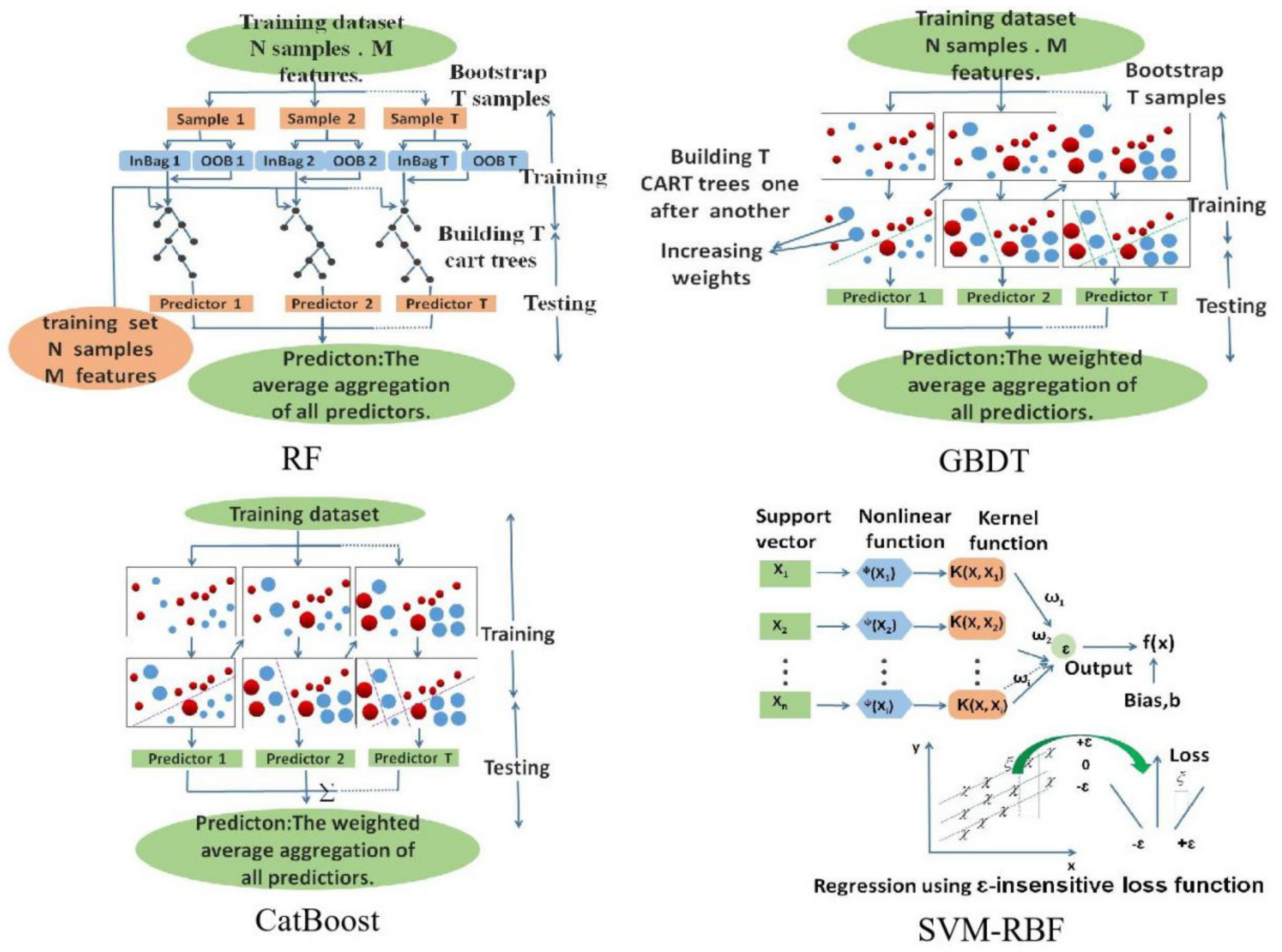
2.3. Tree-Based Ensemble Models

2.3.1. Classification and Regression Trees (CART)

The CART proposed by Breiman et al. [49] is a tree-based nonlinear regression model. More details about the CART model can be found in Breiman et al. [49].

2.3.2. Extremely Randomized Trees (ET)

The extremely randomized trees (or extra trees) model, proposed by Geurts et al. [50] and developed from the RF algorithm, is a tree-based model. The ET algorithm uses the principle to train each base estimator by applying a random subset of features as an RF model. However, the difference between ET and RF is that the latter applies a bootstrap replica to train the algorithm, whereas the former trains each regression tree by employing the whole training dataset. More detailed information about the ET model can be found in Geurts et al. [50].

2.3.3. Random Forest (RF)

The RF algorithm, proposed by Breiman [51], is a bagging-based model that uses a regression tree method. More information about this algorithm can be found in Breiman [51] and the structure of the RF model is shown in Figure 2.

2.3.4. Gradient Boosting Decision Tree (GBDT)

The GBDT algorithm, a tree-based ensemble algorithm, proposed by Friedmen [52], has been widely applied in regression problems. Different from the RF algorithm or traditional single-tree models (such as M5Tree), the GBDT algorithm can reduce biases and yield a combination of trees (Figure 2), while the RF algorithm reduces the variances. The details regarding this algorithm can be found in Friedmen [52] and the structure of the GBDT is shown in Figure 2.

2.3.5. Extreme Gradient Boosting (XGBoost)

The XGBoost algorithm, proposed by Chen and Guestrin [39], is based on the idea of “boost”. The purpose of this idea is to develop a “strong” learner through additive training strategies. The general equation for the estimation at step t is shown as follows:
f i t = k = 1 t f k ( x i ) = f i ( t 1 ) + f t ( x i )
where xi is the input variable and f i ( t ) and f t ( x i ) are the estimations and learner at step t, respectively [41].
To prevent the over-fitting problem without reducing the computing time of this algorithm, the objective function is presented as:
O b j ( t ) = k = 1 n l ( y i ¯ , y i ) + k = 1 t Ω ( f i )
where n denotes the number of observations, l is the loss function and Ω represents the regularization in the form of:
Ω ( f ) = γ T + 1 2 λ ω 2
where γ means the minimum loss needed to further partition the leaf node, λ denotes the regularization parameter and ω represents the vector of scores in the leaves. More details regarding this algorithm can be found in Chen and Guestrin [39].

2.3.6. Gradient Boosting with Categorical Features Support (CatBoost)

The CatBoost model is a newly developed GBDT algorithm [43]. This algorithm has improved considerably compared to the traditional GBDT algorithm. (1) When dealing with categorical features during training, if a permutation exists, it is substituted with:
x σ p , k = j = 1 p 1 x σ j , k = x σ p , k · Y σ j + β · P j = 1 p 1 x σ j , k = x σ p , k + β
where β and P are the weights of the prior value and the prior value, respectively [53]. (2) A new technique, named ordered boosting and proposed by Prokhorenkova et al. (2017), was used to solve the problem of gradient bias. (3) Oblivious trees were applied as base predictors. (4) To avoid over-fitting, a new schema was used to calculate leaf values when selecting the tree structure. More details can be found in Dorogush et al. [43] and the structure of the CatBoost algorithm can be found in Figure 2.

2.3.7. Light Gradient Boosting Method (LightGBM)

The LightGBM algorithm, a newly developed GBDT model [42], can decrease the number of data instances and features. In this algorithm, two novel techniques were proposed to achieve this goal. The first one is Gradient-based One-Side Sampling (GOSS) and it can achieve a good balance between reducing the number of data instances and keeping the accuracy of decision trees. The second one is Exclusive Feature Bunding (EFB) and it can effectively achieve the goal of reducing the number of features.
In the GOSS technique, an instance subset A is obtained by keeping the top-a × 100% instances with smaller gradients, and a subset B with size b × A c randomly sampled; finally, the instances are split according to the estimated variance gain V j ( d ) over the subset A B , i.e.,
V j ( d ) = 1 n ( x i A l g i + 1 a b x i b l g i 2 n l j ( d ) + x i A r g i + 1 b a x i B r g i 2 n r j ( d ) )
where A l = x i A : x i j d , A r = x i A : x i j d , B l = x i B : x i j d , B r = x i B : x i j d , and the coefficient 1 a b is used to normalize the sum of the gradients over B back to the size of Ac [44].
In the proposed EFB method, determining which features should be bundled together and how to construct the bundle are two inevitable issues. Therefore, a greedy algorithm is used, which can produce reasonably good results for graph coloring to produce the bundles for the first issue and a way of merging exclusive features is applied to simplify the training process for the second issue. More details about the LightGBM algorithm can be found in Ke et al. [42].

2.4. Multi-Layer Perceotron (MLP)

The MLP neural network, popularly known as ANN models with the capability of time series prediction, is widely applied in the fields of hydrological cycles and solar radiation [54]. Each MLP model consists of an input layer, hidden layer and output layer. More details about the MLP algorithm can be found in Wang et al. [12].

2.5. Support Vector Machine (SVM)

The SVM model, developed by Vapnik [55], is based on a series of kernel functions, and it has been widely employed in fields such as meteorology, agriculture and hydrology studies. The existing studies found that the Radial Basis Function (RBF), regarded as a kind of non-linear kernel function, performed better in estimating tasks than other kernel models in all type of SVM models [56]. Therefore, in this study, the SVM model based on RBF (SVM-RBF) was applied. More details about the SVM-RBF algorithm can be found in Vapnik [55] and the structure of this algorithm is shown in Figure 2.

2.6. Input Combinations and K-Fold Cross-Validation

Considering the correlations between each input variable and Rs, seven input combinations were employed to access the roles of various meteorological parameters in estimating daily Rs (Table 3): (1) Ra, n/N; (2) Ra, n/N, Tmax, Tmin; (3) Ra, n/N, Ho, U10; (4) Ra, n/N, Pre, Prs; (5) Ra, n/N, Tmax, Tmin, Ho, U10; (6) Ra, n/N, Tmax, Tmin, Pre, Prs; (7) Ra, n/N, Tmax, Tmin, Ho, U10, Pre, Prs. The k-fold cross-validation method was generally applied to make full use of the time series [41]. The whole time series during 1993–2016 was equally divided into four sections in this study. The four cross-validation stages are presented in Table 4. In each simulation, three sections were applied to train the algorithms and the remaining one for validating the algorithms. Therefore, there are four various validating stages in total in this study, and the training and testing results in tables are the mean values of four stages.
The optimization of parameters for various algorithms at each site was a key step in obtaining optimal predictions. The grid search method was selected to optimize key hyper-parameters. The key parameters ranged between their thresholds using the trial-and-error method at a certain interval. All the parameter pairs were tried and the one with the best accuracy was selected for training and testing the model. For example, for the CatBoost model, the number of rounds varied from 200 to 800 at 100 intervals, the maximum tree depth varied between 2 and 10 at 2 intervals, and the subset ratio of all data sets ranged from 0.5 to 1 at 0.05 intervals. More information about the optimization of hyper-parameters can be found in Table 5.
All models were run using Programming language in the Python computing environment (version 3.6). The URLs for the “XGBoost”, “CatBoost” and “LightGBM” package are: https://xgboost.readthedocs.io/en/latest/, https://github.com/catboost/catboost and https://lightgbm.readthedocs.io/en/latest/, respectively (accessed on 1 October 2020). All the computing processes were conducted using a computer with 256 GB of RAM memory and 10×Intel Xeon CPU E5 2650 @ 2.3 GHz, with a Debian x86_64 GNU/Linux operating system.

2.7. Statistical Evaluation
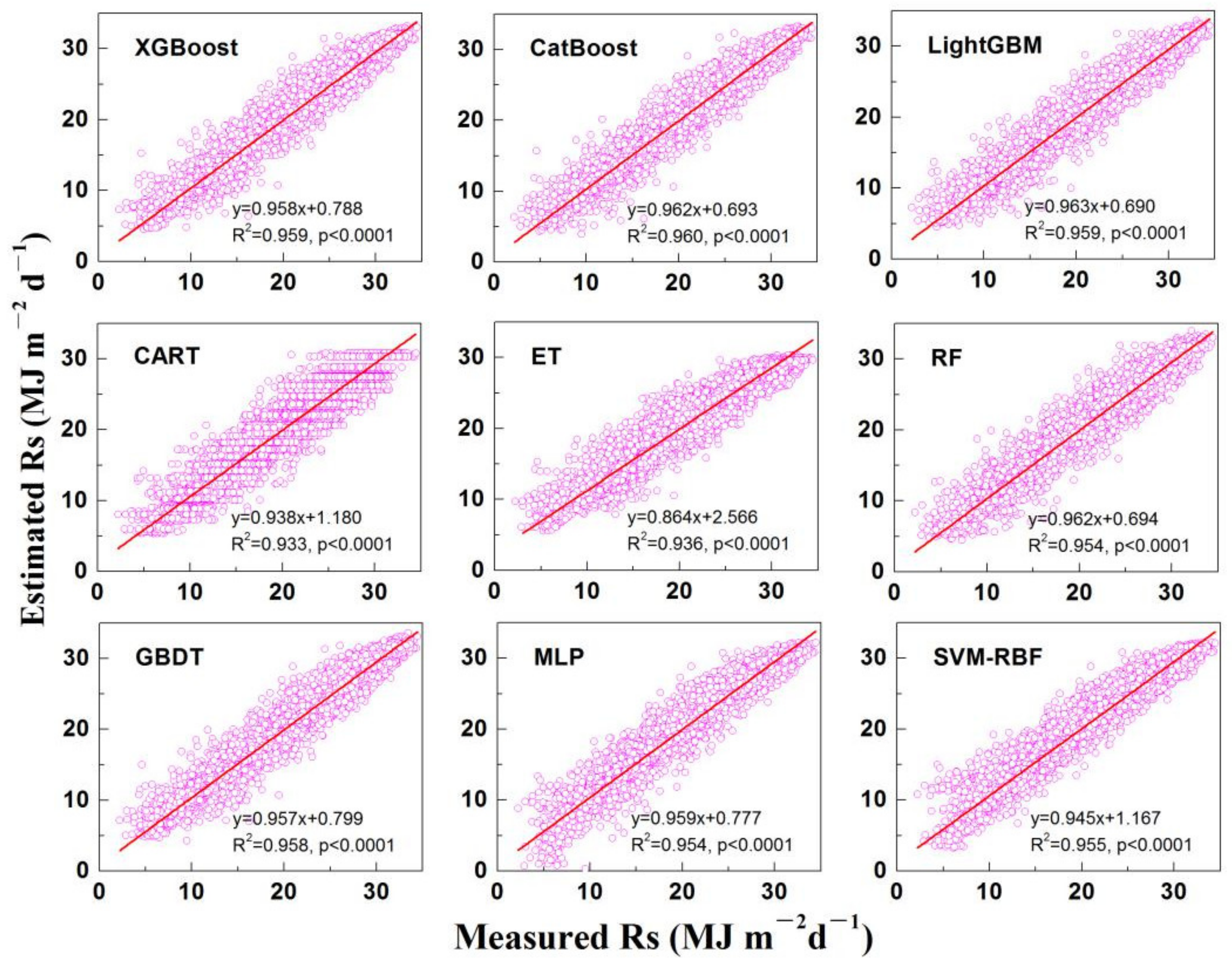
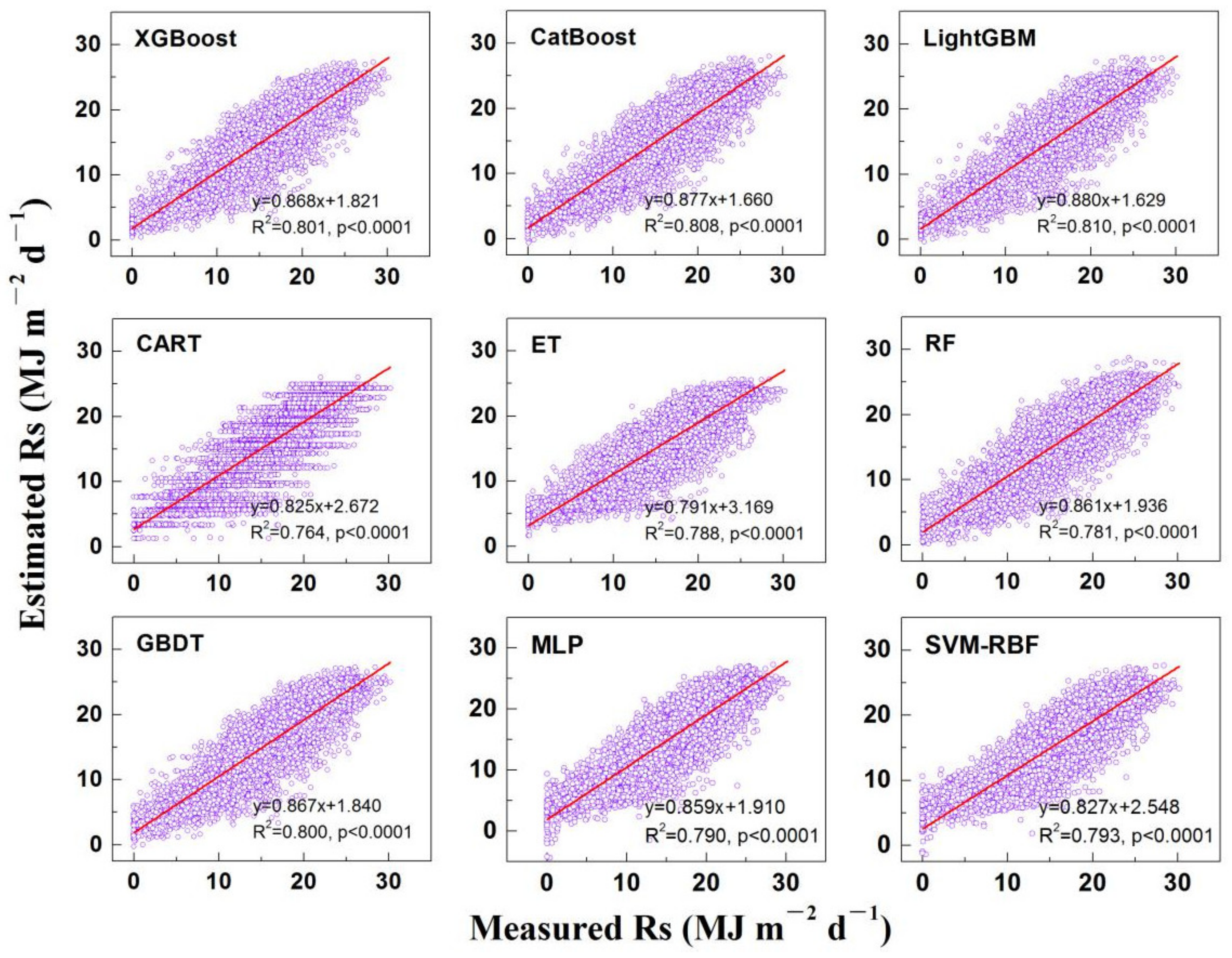
The performances of the developed algorithms for estimating daily Rs are accessed using four statistical indicators, including R2, RMSE, MAE and MBE [22]:
R 2 = i = 1 n ( X m i X m ¯ ) ( X o i X o ¯ ) 2 i = 1 n ( X m i X m ¯ ) 2 i = 1 n ( X o i X o ¯ ) 2
RMSE = 1 n i = 1 n ( X m i X o i ) 2
MAE = 1 n i = 1 n X m i X o i
MBE = 1 n i = 1 n ( X m i X o i )
where n indicates the number of the time series, and Xm and Xo are the simulated and measured daily Rs, respectively.
The raw meteorological variables are normalized using the following equations before applying these algorithms to the time series:
x n = x i x min x max x min
where xi and xn donate the raw and normalized data, respectively; xmin and xmax represent the extreme values of the dataset, respectively; and xn are scaled in the range [0, 1].

3. Results

3.1. Comparison of Model Accuracy under Various Input Combinations

The statistical results of the developed models (CART, ET, RF, GBDT, XGBoost, CatBoost, LightGBM, MLP and SVM-RBF) for estimating daily Rs under the various input combinations during training and testing stages at 16 sites are presented in Supplementary Materials Tables S1–S17. The top three models among the nine models under each input combination are highlighted in bold, red and blue, respectively.
The accuracy of daily Rs estimation differed significantly from various input combinations. Table 6 shows the statistical values of various models with different input combinations during training and testing stages at all stations on average. It’s clear that all models using the complete meteorological dataset (C7) achieved the best accuracy (on average R2 = 0.903, RMSE = 2.091 MJm−2d−1, MAE = 1.579 MJm−2d−1) in comparison to the other incomplete input combinations. Supplementary Materials Figures S1–S16 show the scatter plots of the predicted Rs values using all machine learning models under complete input combinations (C7) at 16 stations. It’s clear that the Geermu station (Figure 3) showed the best testing accuracy using the CatBoost model (R2 = 0.960, RMSE = 1.412 MJm−2d−1, MAE = 1.010 MJm−2d−1). In contrast, Sanya station (Figure 4) had the worst testing accuracy using RF model (R2 = 0.764, RMSE = 2.913 MJm−2d−1, MAE= 2.260 MJm−2d−1). Moreover, it is noteworthy that all models provided acceptable prediction accuracy under C1 (on average R2 = 0.888, RMSE = 2.249 MJm−2d−1, MAE = 1.696 MJm−2d−1), indicating that Ra and n/N had a great influence on daily Rs estimation. Moreover, LightGBM outperformed the XGBoost and GBDT models under C5, C6 and C7, while it performed worse under C1, C2, C3 and C4 (Table 6), which illustrates that LightGBM exhibited better prediction accuracy when more variables were input for daily Rs estimation.

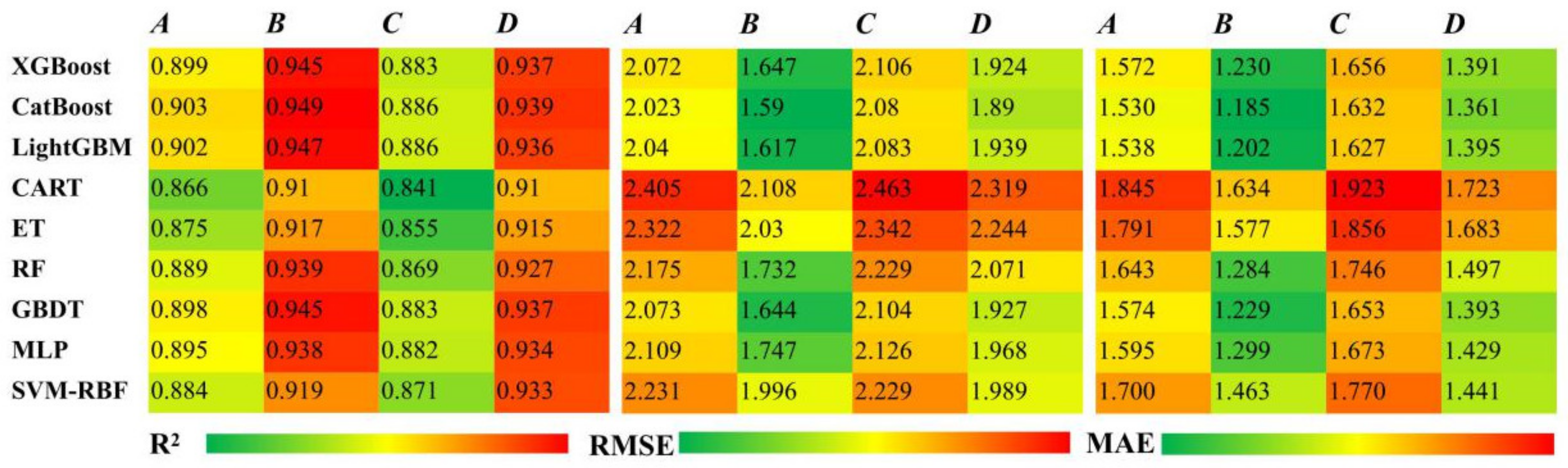
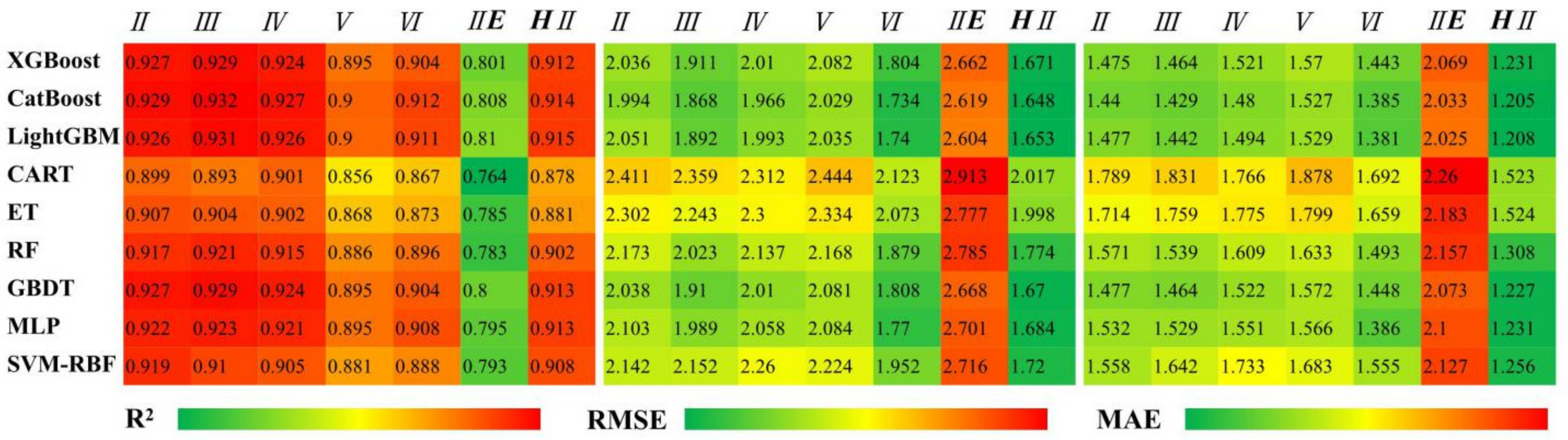
3.2. Comparison of Various Model Accuracy at Different Stations in Various Climatic Zones

To simplify the results of comparison, we select five typical stations in contrasting climatic zones to present the performance of various models (Tables S1, S4, S7, S14 and S16). Table S1 provides the comparisons of the MLP, SVM-RBF and various tree-based ensemble models for Sanya station. This station performed the worst among all stations in humid regions of South China. For example, the R2 values of MLP, SVM-RBF, CART, ET, RF, GBDT, XGBoost, CatBoost and LightGBM models ranged from 0.775–0.795, 0.777–0.798, 0.755–0.782, 0.779–0.797, 0.727–0.791, 0.705–0.806 and 0.739–0.814, respectively; RMSE values ranged from 2.711–2.823, 2.680–2.820, 2.797–2.963, 2.700–2.813, 2.727–3.127, 2.622–2.947 and 2.569–3.046 MJm−2d−1, respectively; and MAE values ranged from 2.105–2.199, 2.095–2.162, 2.184–2.292, 2.124–2.212, 2.125–2.398, 2.043–2.280 and 2.000–2.350 MJm−2d−1, respectively. Table S4 presents the comparisons of all the models at Wuhan station. The R2 values of MLP, SVM-RBF, CART, ET, RF, GBDT and the three newly developed tree-based ensemble models ranged from 0.888–0.910, 0.881–0.897, 0.880–0.895, 0.883–0.892, 0.854–0.903, 0.890–0.915 and 0.887–0.918, respectively; RMSE values ranged from 2.243–2.511, 2.407–2.585, 2.422–2.600, 2.457–2.561, 2.323–2.863, 2.171–2.476 and 2.127–2.511 MJm−2d−1, respectively; and MAE values ranged from 1.655–1.908, 1.808–1.961, 1.831–1.986, 1.885–1.966, 1.735–2.155, 1.614–1.869 and 1.572–1.901 MJm−2d−1, respectively. Table S7 shows the training and testing accuracy of all models at Haerbin station. The R2 values of MLP, SVM-RBF, CART, ET, RF, GBDT and the three newly developed tree-based ensemble models ranged from 0.913–0.924, 0.917–0.922, 0.895–0.897, 0.904–0.908, 0.894–0.921, 0.915–0.928 and 0.913–0.930, respectively; RMSE values ranged from 1.965–2.098, 1.988–2.046, 2.298–2.321, 2.168–2.208, 2.007–2.331, 1.911–2.078 and 1.880–2.103 MJm−2d−1, respectively; and MAE values ranged from 1.450–1.561, 1.471–1.506, 1.720–1.740, 1.625–1.622, 1.484–1.716, 1.424–1.534 and 1.393–1.550 MJm−2d−1, respectively. Table S14 shows the training and testing accuracy of all models at Geermu station in the Plateau and Mountain climatic zones, respectively. The R2 values of the MLP, SVM- RBF, CART, ET, RF, GBDT and the three newly developed tree-based ensemble models ranged from 0.951–0.957, 0.955–0.957, 0.932–0.933, 0.934–0.940, 0.943–0.954, 0.956–0.959 and 0.955–0.961, respectively; RMSE values ranging from 1.465–1.569, 1.461–1.510, 1.838–1.845, 1.738–1.812, 1.515–1.691, 1.440–1.490 and 1.405–1.505 MJm−2d−1, respectively; and MAE values ranging from 1.052–1.122, 1.043–1.068, 1.379–1.382, 1.308–1.379, 1.093–1.205, 1.037–1.069 and 1.010–1.076 MJm−2d−1, respectively. Table S16 presents the comparisons of all models at Ejinaqi station in the arid temperate continental climatic zone. Ejinaqi station had the best performance, with R2 values of MLP, SVM-RBF, CART, ET, RF, GBDT and the three newly developed tree-based ensemble models ranging from 0.946–0.955, 0.951–0.956, 0.933–0.934, 0.929–0.938, 0.937–0.950, 0.950–0.957 and 0.948–0.959, respectively; RMSE values ranging from 1.601–1.744, 1.575–1.667, 1.939–1.948, 1.872–1.997, 1.675–1.881, 1.561–1.680 and 1.522–1.711 MJm−2d−1, respectively; and MAE values ranging from 1.146–1.262, 1.122–1.195, 1.433–1.439, 1.397–1.499, 1.195–1.348, 1.119–1.210 and 1.090–1.226 MJm−2d−1, respectively.
The R2, RMSE and MAE for all models in various climate zones across China are also shown in Figure 5 and Figure 6, respectively. The CatBoost, LightGBM, XGBoost and GBDT model significantly outperformed the other models in different humidity and temperature zones. Moreover, all the models showed the highest accuracy with R2 ranging from 0.910 to 0.949, RMSE ranging from 1.590 to 2.108 MJm−2d−1 and MAE ranging from 1.185 to 1.634 MJm−2d−1 in the semi-humid zone, while the lowest accuracy was observed in the semi-arid zone, with R2 ranging from 0.841 to 0.886, RMSE ranging from 2.080 to 2.463 MJ m−2d−1 and MAE ranging from 1.627 to 1.923 MJm−2d−1. Furthermore, all the models performed better in mid-temperate, warm temperate and north subtropical zones, with R2 ranging from 0.893 to 0.931, RMSE ranging from 1.868 to 2.411 MJm−2d−1 and MAE ranging from 1.429 to 1.831 MJm−2d−1, respectively, while the lowest accuracy was observed in the mid-tropical zone, with R2 ranging from 0.764 to 0.810, RMSE ranging from 2.604 to 2.913 MJm−2d−1 and MAE ranging from 2.025 to 2.260 MJm−2d−1. The above analyses clearly show that the CatBoost model generally provided the best accuracy in estimating Rs at different stations or in various climatic zones, followed by the LightGBM, XGBoost, GBDT, MLP, RF, SVM-RBF, ET and CART models.

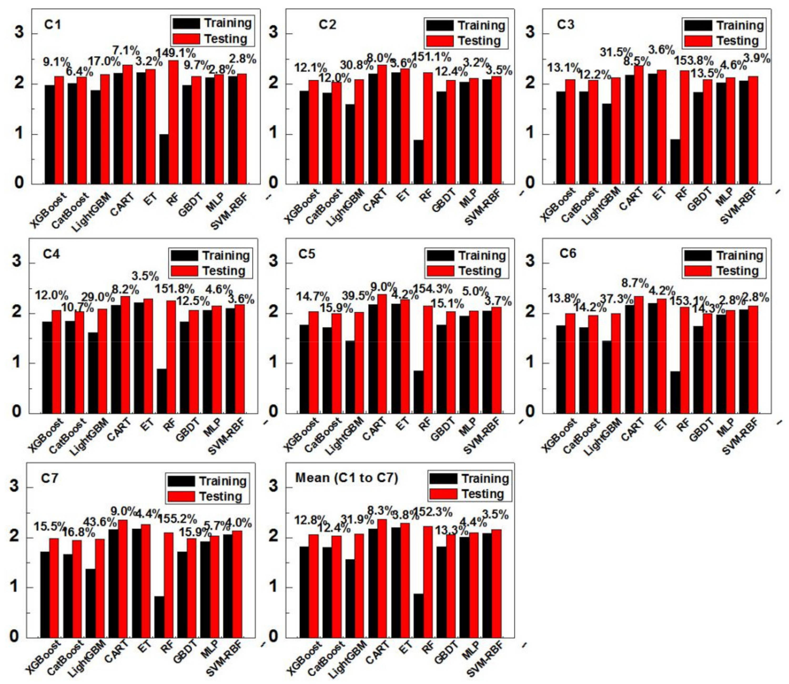
3.3. Comparison of Stability of Various Models

The RF and LightGBM models performed significantly superior to the other models in the training stage (marked in red or bold in Tables S1–S16). However, the CatBoost and LightGBM models generally performed better than the other models in the testing stage, and the GBDT and XGBoost models also provided comparable performances to the CatBoost and LightGBM models (marked in bold or colors in Tables S1–S16). The mean training and testing RMSE of 16 stations are shown in Figure 7 for all models under various input combinations. It was obvious that the three newly developed tree-based ensemble models (CatBoost, LightGBM, XGboost) and GBDT model had the best prediction accuracy in the testing stage for all input combinations, whereas the CART, ET and RF provided higher RMSE values. Meanwhile, the increasing percentage in testing RMSE over training RMSE (average for all sixteen stations) under seven input combinations is also exhibited in Figure 7. The figure indicates that ET, MLP and SVM-RBF models were the most stable models with smallest increases in testing RMSE (from 3.5% to 4.4%). On the contrary, the RF model was the most unstable model with the largest increase in testing RMSE (152.3%). This suggested that the RF model encountered a serious over-fitting problem. Moreover, the CART, GBDT, XGBoost, CatBoost and LightGBM models also showed acceptable percentage increases (on average, from 8.3% to 31.9%) in testing RMSE, indicating that the above models didn’t encounter an over-fitting problem and had comparable model stability.

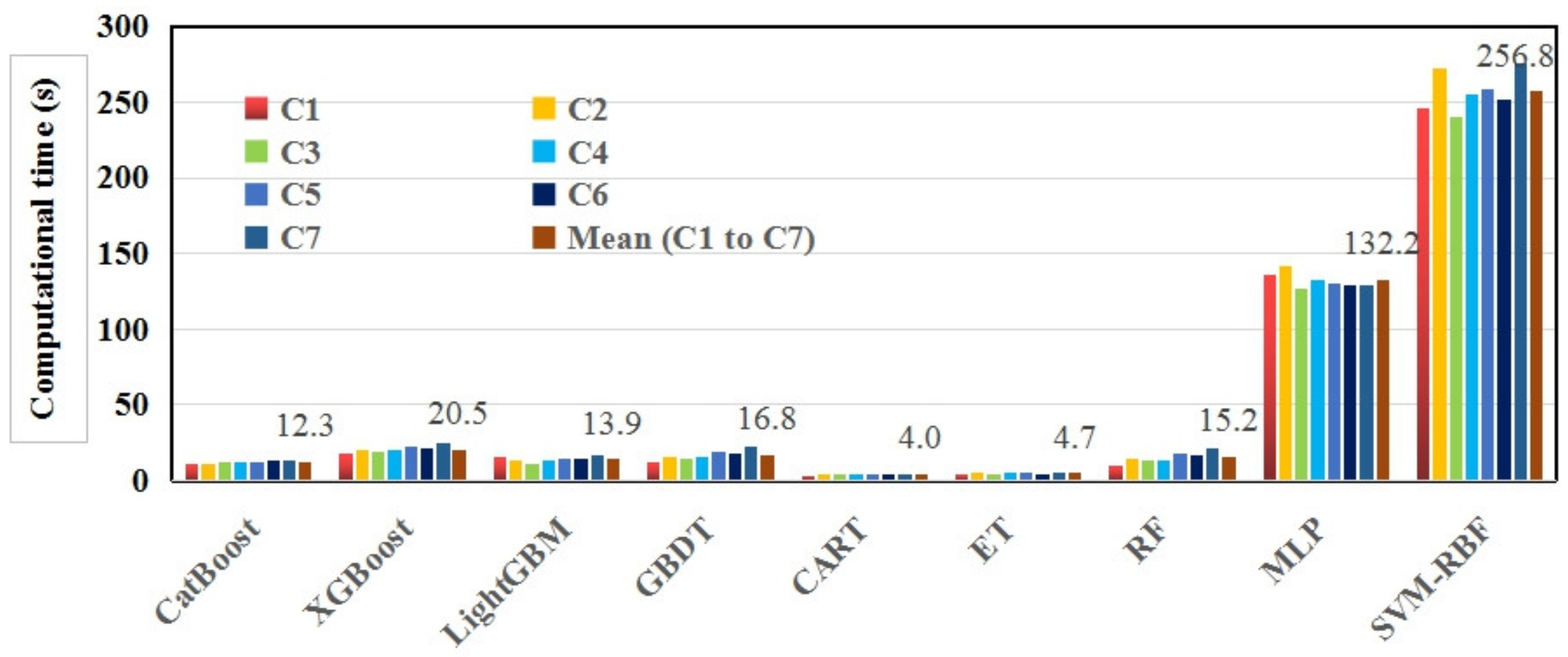
3.4. Computational Costs of Various Models

Figure 8 shows the average computational time of the various developed algorithms under seven various input combinations for all stations in training stages in the Python computing environment (version 3.6). It is clear that the average computational time cost by the SVM-RBF (256.8 s) and MLP (132.1 s) were much higher than the other tree-based ensemble models (less than 21 s) under seven input combinations. In particularly, CART and ET showed the highest computational efficiency with 4 s and 4.7 s, respectively. Meanwhile, CatBoost, LightGBM, XGBoost, GBDT and RF also showed comparable computational efficiency (from 12.3 s to 20.5 s) to CART and ET. In general, it is clear that the average computational time depends on the specific model.

4. Discussion

4.1. Input Combination Strategy of Meteorological Parameters

The results obtained from the above models indicates that the more complete the input variables are, the more accurate the prediction accuracy. However, different meteorological parameters may play various roles in estimating Rs in different climatic zones. For example, the present study indicates that Tmax and Tmin, or Pre and Prs, were more important than Ho and U10 for Rs estimation. Fan et al. [32] revealed that the machine learning methods with Tmax, Tmin and Pre obtained acceptable Rs estimation in central and southern China with a humid subtropical climate. This also illustrated that the more appropriate the input combinations are, the more accurate the prediction accuracy. Moreover, previous studies had demonstrated that sunshine duration (n/N) and Ra were the most significant input variables in estimating daily Rs, compared to those based on air temperature or other single meteorological parameters [57], which explains why the models based on only n/N and Ra (C1) could also produce acceptable prediction accuracy (on average, R2 = 0.888, RMSE = 2.249 MJm−2d−1, MAE = 1.696 MJm−2d−1) in different stations in our study. Moreover, previous studies also indicated that temperature-based models could obtain comparable prediction accuracy for estimating Rs [58,59]. For instance, Fan et al. [6] proposed six new temperature-based models for daily Rs estimation at 20 solar radiation stations in the humid subtropical and tropical regions of China. The results showed that R2 values ranged 0.65–0.78, which explained why Tmax and Tmin played more significant roles in modeling Rs than Ho and U2.

4.2. Prediction Accuracy of Various Models in Various Climatic Zones

Previous studies had found that the most appropriate model for each station differed in various climatic zones [60]. For example, Wu et al. [38] revealed that the CatBoost model performed better than MARS, RF, MLP M5tree for daily Rs estimation at four stations in South China with the R2 ranging 0.887–0.939, RMSE ranging 1.916–2.648 MJm−2d−1 and MAE ranging 1.451–1.873 MJm−2d−1 under complete input combination, which was in agreement with our findings. Chen et al. [4] also found that M5tree outperformed BP, GRNN, MARS and GA for estimating daily DHI across China with the R2 ranging 0.824–0.914. Zou et al. [61] also found that the ANFIS model performed better than the improved Bristow-Campbell model and Yang’s Hybrid model for daily Rs estimations at three stations in Hunan province of China, with the R2, RMSE and MAE values for ANFIS model ranging 0.79–0.86, 2.75–3.90 MJm−2d−1 and 2.08–2.62 MJm−2d−1, respectively. However, the CatBoost, LightGBM, XGBoost and GBDT models were always ranked first, second, third and fourth, respectively, in terms of prediction accuracy in all climatic zones or stations in this study, and this indicated that the three newly developed tree-based ensemble models (CatBoost, LightGBM, XGBoost) had general applicability in various climatic zones of China. Moreover, the station with the highest accuracy was Geermu station with an arid and plateau temperate zone, due to the scarce water vapor and clouds, as well as a thin atmosphere, leading to a weak radiative attenuation process. On the contrary, Sanya station, with a humid and midtropical zone, had the worst accuracy, perhaps attributed to adequate water vapor, clouds and a complex radiative attenuation process. It should be noted that Wulumiqi, Chengdu and Lasa stations also exhibited worse accuracy compared to the other stations, which might result from the high atmospheric dust loading for Wulumiqi station, basin topography for Chengdu station and valley topography for Lasa station. For example, Chengdu station is located in Sichuan basin, where water vapor and clouds are not easily dispersed, due to sealed terrain. Lasa station lies in Lasa River valley where humidity and precipitation are relatively more sufficient than Geermu, although they are all located in Qinghai-Tibet Plateau. In general, one significant reason for the various model performances in different climatic zones was related to the local climatic and geographical conditions at each station. Moreover, the prediction accuracy of various models significantly differed from one station to another due to the differences in the local microclimate, even if they were located in same climatic zone.

4.3. Stability of Various Models

The stability of all models was also considered as a vital indicator when estimating Rs. The results showed that the RF model exhibited the largest percentage increase in testing RMSE compared to the other models in this study. Hassan et al. [59] had also revealed that the RF exhibited a larger increase in testing RMSE over training RMSE than the SVM and tree-based ensemble models for estimating Rs. Huang et al. [53] also found that the RF model exhibited a larger percentage increase in MAPE and RMSE than the SVM and CatBoost models for estimating ETo. This illustrated that RF was inferior for regression problems, despite the fact that it performed well for classification problems. Due to the RF model not being able to make a prediction beyond the range of the training dataset, an over-fitting problem arises when noisy data in the testing stage are employed for prediction. On the contrary, the MLP, SVM-RBF and ET models showed the best model stability with the smallest percentage increase in RMSE and successfully avoided the over-fitting problem. Fan et al. [41] revealed that SVM was the most stable model compared to the XGBoost, GBDT, M5Tree and RF models, which was in agreement with our findings. In addition, CART, GBDT, XGBoost, CatBoost and LightGBM also exhibited comparable model stabilities as MLP, SVM-RBF and ET in this study, because the successive trees can reduce the errors incorrectly predicted by the earlier predictors using extra weight, and a weight vote is finally adopted for estimation [62].

4.4. Computational Costs of Various Models under Different Input Combinations

The data size used in this study was relatively small, which led to relatively small differences in computational time among the six tree-based ensemble models (CART, ET, RF, GBDT, XGBoost, LightGBM and CatBoost). However, the time differences between the seven models and the other three models (SVM-RBF and MLP) would be much larger when more variables, more stations, a smaller time scale and longer time series were applied to develop a general model. For example, it would show enormous computational time differences when more than 2400 meteorological stations at a three-hour scale from 2001–2017 in China were used to develop the models. Therefore, computational efficiency was also considered as a vital indicator when estimating Rs. The present study exhibits that the CART, ET, RF, GBDT, XGBoost, LightGBM and CatBoost models had higher computational efficiency than the SVM-RBF and MLP models in the Python computing environment (version 3.6). The previous studies had also revealed that the computational time of the SVM model was 39 times the computational time of the RF model [59]. Wu et al. [38] argued that the CatBoost model exhibited the highest computational efficiency compared to MLP, M5Tree, MARS, RF and KNBA models in the R computing environment, and Huang et al. [53] also found that the average time consumed by the CatBoost model in the R computing environment was much less than that of the RF or the SVM model when estimating ETo. The high computational efficiency of the CatBoost, LightGBM, RF and XGBoost models was largely due to the advantage that they could be trained in parallel, and CART provided the fastest computing time because it was a single-tree model.

4.5. Comprehensive Evaluation of Various Models

Considering the above analysis comprehensively, the priority of the MLP, SVM-RBF and seven tree-based ensemble algorithms could be ranked as follows: CatBoost > LightGBM > XGboost > GBDT > SVM-RBF > MLP > RF > ET > CART. When it came to model stability, the nine models could be sorted as follows: SVM-RBF > ET > MLP > CART > CatBoost > XGboost > GBDT > LightGBM > RF. Similarly, the nine models could be ordered in terms of their computational time: CART > ET > CatBoost > LightGBM > RF > GBDT > XGBoost > MLP > SVM-RBF. The CatBoost, LightGBM, XGboost and GBDT models exhibited the best prediction accuracy, acceptable stability and computational time among all models in this study. Meanwhile, although the CART and ET models exhibited good stability and fastest computational speeds, their prediction accuracy performed worst among all models. Therefore, it was the CatBoost, LightGBM, XGBoost and GBDT models, not the CART and ET models, that could be recommended for estimating daily Rs in this study. This also demonstrated that the CatBoost, LightGBM, XGBoost and GBDT models should be considered as promising artificial intelligence algorithms based on model stability, computational time and prediction accuracy in the Python computing environment for estimating Rs in various climatic zones of China and possibly elsewhere in the world with similar climatic zones (e.g., southeastern United States, southeast Australia, southern Japan and South Korea for subtropical monsoon climates; northern Japan and North Korea for temperate monsoon climates; Southeast Asia and India for tropical monsoon climates; Central Asia for the temperate continental climate; and western America for plateau and mountain climates).

5. Conclusions

This study developed the three new tree-based ensemble models (XGBoost, LightGBM and CatBoost) for estimating daily Rs using eight input variables (Ra, n/N, Tmax, Tmin, Ho, U10, Pre and Prs) under seven input combinations at 16 stations in different climatic zones of China during 1993–2016. The three newly developed tree-based ensemble models were also compared to the other four common tree-based ensemble models (CART, ET, RF and GBDT), one kernel-based model (SVM-RBF) and one artificial neural network model (MLP), comprehensively considering prediction accuracy, model stability and computational time. The three newly developed tree-based ensemble models (LightGBM, CatBoost and XGBoost) and GBDT model offered a better prediction accuracy than the other models and acceptable model stability and computational time in the Python computing environment. Moreover, the more complete the input variables, the more accurate the estimation accuracy, with extra-terrestrial solar radiation (Ra) and sunshine duration (C1) the most important influencing factors on daily Rs estimation when applying these models to estimate Rs.
Thus, the three newly developed tree-based ensemble models (CatBoost, LightGBM and XGBoost) and the GBDT model are highly recommended as promising alternative models for estimating daily Rs at various stations in different climatic zones of China, comprehensively considering prediction accuracy, stability and computational efficiency in the Python computing environment.
Further investigations are required to evaluate and compare computational costs for all models in R, Matlab, Fortran or other computing environments. Moreover, it is also required to evaluate the performances of newly developed tree-based ensemble models under various input combinations at monthly and hourly time scales in various climates of China and elsewhere worldwide with similar climatic zones (e.g., southeastern United States, southeast Australia, southern Japan and South Korea for subtropical monsoon climates, northern Japan and North Korea for temperate monsoon climates, Southeast Asia and India for tropical monsoon climates, Central Asia for the temperate continental climate and western America for plateau and mountain climates) in our subsequent work. Furthermore, more attention should also be paid to mapping the regional and global radiation distribution at a high spatial resolution by combining remote sensing techniques and machine learning models.

Supplementary Materials

The following supporting information can be downloaded at: https://www.mdpi.com/article/10.3390/en15093463/s1.

Author Contributions

Conceptualization, Z.Z. and L.H.; methodology, A.L.; software, Z.Z.; validation, Z.Z. and L.W.; writing—original draft preparation, Z.Z.; writing—review and editing, L.H.; visualization, Z.Z.; supervision, A.L.; funding acquisition, L.H. All authors have read and agreed to the published version of the manuscript.

Funding

This research was funded by basic scientific research business expenses of Central University, grant number 2662021GGQD002.

Data Availability Statement

Not applicable.

Acknowledgments

We would like to thank the China Meteorological Administration (CMA) for providing the meteorological and solar radiation data (http://data.cma.cn, accessed on 1 October 2020).

Conflicts of Interest

The authors declare no conflict of interest.

Nomenclature

RsGlobal solar radiation/solar energy resource potential (MJ m−2)
RaExtra-terrestrial solar radiation (MJ m−2)
DHIDirect horizontal irradiance (MJ m−2)
PARPhotosynthetically active radiation (MJ m−2)
nObserved sunshine duration (h)
NMaximum possible sunshine duration (h)
TAir temperature (°C)
TaAnnual mean air temperature (°C)
TmaxMaximum temperature (°C)
TminMinimum temperature (°C)
HrRelative humidity (%)
PrePrecipitation (mm)
U10Wind speed at 10 m height (ms−1)
PrsPressure (hpa)
EToReference evapotranspiration (mm)
RDetermination coefficient
RMSERoot mean square error
MAEMean absolute error
MBEMean bias error
SVMSupport vector machine
ANNArtificial neural network
MLPMulti-layer perceptron
ANFISAdaptive neuro fuzzy inference system
TBAMTree-based assemble mode
RFRandom forest
GBDTGradient boosting decision tree
XGBoostExtreme gradient boosting
CatBoostGradient boosting with categorical features support
LightGBMLight gradient boosting method
ANFIS-GPANFIS with grid partition
ANFIS-SCANFIS with subtractive clustering

Appendix A

The extra-terrestrial solar radiation (Ra) and maximum possible sunshine duration (N) were obtained using following equations:
R a = 24 / π × I s c ( 1 + 0.033 cos 360 N d 365 ) × π W S 180 sin δ sin φ + cos δ cos φ sin W S
δ = 23.45 sin [ 360 × ( 284 + N d ) / 365 ]
W S = cos 1 ( tan δ tan φ )
N = 2 15 cos 1 tan ( δ ) tan ( φ )
where I s c is the solar constant (1367 Wm−2), δ indicates the solar declination, φ represents the latitude of the location, W S denotes hour angle, and N d means the day of the year starting from January 1st.

References

  1. Wild, M. Enlightening Global Dimming and Brightening. Bull. Am. Meteorol. Soc. 2012, 93, 27–37. [Google Scholar] [CrossRef]
  2. The International Renewable Energy Agency. Renewable Energy Statistics; IRENA: Masdar, United Arab Emirates, 2019. [Google Scholar]
  3. China National Renewable Energy Centre. China Wind, Solar and Bioenergy Roadmap, 2050; CNREC: Beijing, China, 2014. [Google Scholar]
  4. Chen, F.; Zhou, Z.; Lin, A.; Niu, J.; Qin, W.; Zhong, Y. Evaluation of Direct Horizontal Irradiance in China Using a Physically-Based Model and Machine Learning Methods. Energies 2019, 12, 150. [Google Scholar] [CrossRef] [Green Version]
  5. Wang, Y.; Wild, M. A new look at solar dimming and brightening in China. Geophys. Res. Lett. 2016, 43, 11777–11785. [Google Scholar] [CrossRef]
  6. Fan, J.; Chen, B.; Wu, L.; Zhang, F.; Lu, X.; Xiang, Y. Evaluation and development of temperature-based empirical models for estimating daily global solar radiation in humid regions. Energy 2018, 144, 903–914. [Google Scholar] [CrossRef]
  7. Ehnberg, J.; Bollen, M. Simulation of global solar radiation based on cloud observations. Sol. Energy 2005, 78, 157–162. [Google Scholar] [CrossRef]
  8. Fan, J.; Wang, X.; Wu, L.; Zhang, F.; Bai, H. New combined models for estimating daily global solar radiation based on sunshine duration in humid regions: A case study in South China. Energy Convers. Manag. 2018, 156, 618–625. [Google Scholar] [CrossRef]
  9. Zang, H.; Cheng, L.; Ding, T.; Cheung, K.W.; Wang, M.; Wei, Z.; Sun, G. Estimation and validation of daily global solar radiation by day of the year-based models for different climates in China. Renew. Energy 2019, 135, 984–1003. [Google Scholar] [CrossRef]
  10. Chukwujindu, N.S. A comprehensive review of empirical models for estimating global solar radiation in Africa. Renew. Sustain. Energy Rev. 2017, 78, 955–995. [Google Scholar] [CrossRef]
  11. Chen, J.; He, L.; Yang, H.; Ma, M.; Chen, Q.; Wu, S.J.; Xiao, Z.L. Empirical models for estimating monthly global solar radiation: A most comprehensive review and comparative case study in China. Renew. Sustain. Energy Rev. 2019, 108, 91–111. [Google Scholar] [CrossRef]
  12. Wang, L.; Kisi, O.; Zounemat-Kermani, M.; Salazar, G.A.; Zhu, Z.; Gong, W. Solar radiation prediction using different techniques: Model evaluation and comparison. Renew. Sustain. Energy Rev. 2016, 61, 384–397. [Google Scholar] [CrossRef]
  13. Gueymard, C.A. Direct solar transmittance and irradiance predictions with broadband models. Part I: Detailed theoretical performance assessment. Sol. Energy 2003, 74, 355–379. [Google Scholar] [CrossRef]
  14. Gueymard, C.A. Direct solar transmittance and irradiance predictions with broadband models. Part II: Validation with high-quality measurements. Sol. Energy 2003, 74, 381–395. [Google Scholar] [CrossRef]
  15. Yang, K.; Huang, G.; Tamai, N. A hybrid model for estimating global solar radiation. Sol. Energy 2001, 70, 13–22. [Google Scholar] [CrossRef]
  16. Yang, K.; Koike, T.; Ye, B. Improving estimation of hourly, daily, and monthly solar radiation by importing global data sets. Agric. For. Meteorol. 2006, 137, 43–55. [Google Scholar] [CrossRef]
  17. Qin, J.; Tang, W.; Yang, K.; Lu, N.; Niu, X.; Liang, S. An efficient physically based parameterization to derive surface solar irradiance based on satellite atmospheric products. J. Geophys. Res. Atmos. 2015, 120, 4975–4988. [Google Scholar] [CrossRef]
  18. Sun, Z.; Liu, J.; Zeng, X.; Liang, H. Parameterization of instantaneous global horizontal irradiance: Cloudy-sky component. J. Geophys. Res.-Atmos. 2012, 117, D1402. [Google Scholar] [CrossRef] [Green Version]
  19. Sun, Z.; Liu, A. Fast scheme for estimation of instantaneous direct solar irradiance at the Earth’s surface. Sol. Energy 2013, 98, 125–137. [Google Scholar] [CrossRef]
  20. Tang, W.; Yang, K.; Sun, Z.; Qin, J.; Niu, X. Global Performance of a Fast Parameterization Scheme for Estimating Surface Solar Radiation from MODIS Data. IEEE Trans. Geosci. Remote 2017, 55, 3558–3571. [Google Scholar] [CrossRef]
  21. Qin, W.; Wang, L.; Zhang, M.; Niu, Z.; Hu, B. First Effort at Constructing a High-Density Photosynthetically Active Radiation Dataset during 1961–2014 in China. J. Clim. 2019, 32, 2761–2780. [Google Scholar] [CrossRef]
  22. Guermoui, M.; Melgani, F.; Danilo, C. Multi-step ahead forecasting of daily global and direct solar radiation: A review and case study of Ghardaia region. J. Clean. Prod. 2018, 201, 716–734. [Google Scholar] [CrossRef]
  23. Kaba, K.; Sarıgül, M.; Avcı, M.; Kandırmaz, H.M. Estimation of daily global solar radiation using deep learning model. Energy 2018, 162, 126–135. [Google Scholar] [CrossRef]
  24. Sun, Y.; Szucs, G.; Brandt, A.R. Solar PV output prediction from video streams using convolutional neural networks. Energy Environ. Sci. 2018, 11, 1811–1818. [Google Scholar] [CrossRef]
  25. Vakili, M.; Sabbagh-Yazdi, S.R.; Khosrojerdi, S.; Kalhor, K. Evaluating the effect of particulate matter pollution on estimation of daily global solar radiation using artificial neural network modeling based on meteorological data. J. Clean. Prod. 2017, 141, 1275–1285. [Google Scholar] [CrossRef]
  26. Yadav, A.K.; Chandel, S.S. Solar energy potential assessment of western Himalayan Indian state of Himachal Pradesh using J48 algorithm of WEKA in ANN based prediction model. Renew. Energy 2015, 75, 675–693. [Google Scholar] [CrossRef]
  27. Heng, J.; Wang, J.; Xiao, L.; Lu, H. Research and application of a combined model based on frequent pattern growth algorithm and multi-objective optimization for solar radiation forecasting. Appl. Energy 2017, 208, 845–866. [Google Scholar] [CrossRef]
  28. Mousavi, S.M.; Mostafavi, E.S.; Jiao, P. Next generation prediction model for daily solar radiation on horizontal surface using a hybrid neural network and simulated annealing method. Energy Convers. Manag. 2017, 153, 671–682. [Google Scholar] [CrossRef]
  29. Deo, R.C.; Wen, X.H.; Qi, F. A wavelet-coupled support vector machine model for forecasting global incident solar radiation using limited meteorological dataset. Appl. Energy 2016, 168, 568–593. [Google Scholar] [CrossRef]
  30. Wang, L.; Hu, B.; Kisi, O.; Zounemat-Kermani, M.; Gong, W. Prediction of diffuse photosynthetically active radiation using different soft computing techniques. Q. J. R. Meteorol. Soc. 2017, 143, 2235–2244. [Google Scholar] [CrossRef]
  31. Ahmad, M.W.; Reynolds, J.; Rezgui, Y. Predictive modelling for solar thermal energy systems: A comparison of support vector regression, random forest, extra trees and regression trees. J. Clean. Prod. 2018, 203, 810–821. [Google Scholar] [CrossRef]
  32. Fan, J.; Wu, L.; Zhang, F.; Cai, H.; Ma, X.; Bai, H. Evaluation and development of empirical models for estimating daily and monthly mean daily diffuse horizontal solar radiation for different climatic regions of China. Renew. Sustain. Energy Rev. 2019, 105, 168–186. [Google Scholar] [CrossRef]
  33. Fan, J.; Wu, L.; Zhang, F.; Cai, H.; Zeng, W.; Wang, X.; Zou, H. Empirical and machine learning models for predicting daily global solar radiation from sunshine duration: A review and case study in China. Renew. Sustain. Energy Rev. 2019, 100, 186–212. [Google Scholar] [CrossRef]
  34. Yagli, G.M.; Yang, D.; Srinivasan, D. Automatic hourly solar forecasting using machine learning models. Renew. Sustain. Energy Rev. 2019, 105, 487–498. [Google Scholar] [CrossRef]
  35. Voyant, C.; Motte, F.; Notton, G.; Fouilloy, A.; Nivet, M.L.; Duchaud, J.L. Prediction intervals for global solar irradiation forecasting using regression trees methods. Renew. Energy 2018, 126, 332–340. [Google Scholar] [CrossRef] [Green Version]
  36. Yang, L.; Zhang, X.; Liang, S.; Yao, Y.; Jia, K.; Jia, A. Estimating Surface Downward Shortwave Radiation over China Based on the Gradient Boosting Decision Tree Method. Remote Sens. 2018, 10, 185. [Google Scholar] [CrossRef] [Green Version]
  37. Jumin, E.; Basaruddin, F.B.; Yusoff, Y.; Latif, S.D.; Ahmed, A.N. Solar radiation prediction using boosted decision tree regression model: A case study in Malaysia. Environ. Sci. Pollut. Res. 2021, 28, 26571–26583. [Google Scholar] [CrossRef]
  38. Wu, L.; Huang, G.; Fan, J.; Zhang, F.; Wang, X.; Zeng, W. Potential of kernel-based nonlinear extension of Arps decline model and gradient boosting with categorical features support for predicting daily global solar radiation in humid regions. Energy Convers. Manag. 2019, 183, 280–295. [Google Scholar] [CrossRef]
  39. Chen, T.; Guestrin, C. XGBoost: A Scalable Tree Boosting System. In Proceedings of the 22nd ACM SIGKDD International Conference, San Francisco, CA, USA, 13–17 April 2016; Association for Computing Machinery: New York, NY, USA, 2016. [Google Scholar]
  40. Zhou, Z.; Zhao, L.; Lin, A.; Qin, W.; Lu, Y.; Li, J.; Zhong, Y.; He, L. Exploring the potential of deep factorization machine and various gradient boosting models in modeling daily reference evapotranspiration in China. Arab. J. Geosci. 2020, 13, 1287. [Google Scholar] [CrossRef]
  41. Fan, J.; Yue, W.; Wu, L.; Zhang, F.; Cai, H.; Wang, X.; Lu, X.; Xiang, Y. Evaluation of SVM, ELM and four tree-based ensemble models for predicting daily reference evapotranspiration using limited meteorological data in different climates of China. Agric. For. Meteorol. 2018, 263, 225–241. [Google Scholar] [CrossRef]
  42. Ke, G.; Meng, Q.; Finley, T.; Wang, T.; Chen, W.; Ma, W.; Ye, Q.; Liu, T. LightGBM: A Highly Efficient Gradient Boosting Decision Tree. In Proceedings of the 31st Conference on Neural Information Processing Systems, Long Beach, CA, USA, 4–9 December 2017; Curran Associates Inc.: Red Hook, NY, USA, 2017. [Google Scholar]
  43. Dorogush, A.V.; Ershov, V.; Gulin, A. CatBoost: Gradient boosting with categorical features support. arXiv 2018, arXiv:1810.11363. [Google Scholar]
  44. Cao, Y.; Gui, L. Multi-Step wind power forecasting model Using LSTM networks, Similar Time Series and LightGBM. In Proceedings of the 2018 5th International Conference on Systems and Informatics (ICSAI), Nanjing, China, 10–12 November 2018; IEEE: Piscataway, NJ, USA, 2018. [Google Scholar]
  45. Wang, K. Measurement Biases Explain Discrepancies between the Observed and Simulated Decadal Variability of Surface Incident Solar Radiation. Sci. Rep. 2014, 4, 6144. [Google Scholar] [CrossRef] [Green Version]
  46. Wang, K.; Ma, Q.; Li, Z.; Wang, J. Decadal variability of surface incident solar radiation over China: Observations, satellite retrievals, and reanalyses. J. Geophys. Res. Atmos. 2015, 120, 6500–6514. [Google Scholar] [CrossRef]
  47. Shi, G.Y.; Hayasaka, T.; Ohmura, A.; Chen, Z.; Wang, B.; Zhao, J.; Che, H.; Xu, L. Data Quality Assessment and the Long-Term Trend of Ground Solar Radiation in China. J. Appl. Meteorol. Clim. 2008, 47, 1006–1016. [Google Scholar] [CrossRef]
  48. Vamvakas, L.; Salamalikis, V.; Kazantzidis, A. Evaluation of enhancement events of global horizontal irradiance due to clouds at Patras, South-West Greece. Renew. Energy 2020, 151, 764–771. [Google Scholar] [CrossRef]
  49. Breiman, L.; Friedman, J.H.; Olshen, R.A.; Stone, C.J. Classification and Regression Trees (CART). Biometrics 1984, 40, 358. [Google Scholar]
  50. Geurts, P.; Ernst, D.; Wehenkel, L. Extremely randomized trees. Mach. Learn. 2006, 63, 3–42. [Google Scholar] [CrossRef] [Green Version]
  51. Breiman, L. Random Forests—Random Features. Mach. Learn. 1999, 45, 5–32. [Google Scholar] [CrossRef] [Green Version]
  52. Friedman, J.H. Stochastic gradient boosting. Comput. Stat. Data Anal. 2002, 38, 367–378. [Google Scholar] [CrossRef]
  53. Huang, G.; Wu, L.; Ma, X.; Zhang, W.; Fan, J.; Yu, X.; Zeng, W.; Zhou, H. Evaluation of CatBoost method for prediction of reference evapotranspiration in humid regions. J. Hydrol. 2019, 574, 1029–1041. [Google Scholar] [CrossRef]
  54. Khelifi, R.; Guermoui, M.; Rabehi, A.; Lalmi, D. Multi-step-ahead forecasting of daily solar radiation components in the Saharan climate. Int. J. Ambient Energy 2020, 41, 707–715. [Google Scholar] [CrossRef]
  55. Vapnik, V.N. The Nature of Statistical Learning Theory; Springer Science & Business Media: Berlin/Heidelberg, Germany, 2013. [Google Scholar]
  56. Quej, V.H.; Almorox, J.; Arnaldo, J.A.; Saito, L. ANFIS, SVM and ANN soft-computing techniques to estimate daily global solar radiation in a warm sub-humid environment. J. Atmos. Sol. Terr. Phys. 2017, 155, 62–70. [Google Scholar] [CrossRef] [Green Version]
  57. Despotovic, M.; Nedic, V.; Despotovic, D.; Cvetanovic, S. Review and statistical analysis of different global solar radiation sunshine models. Renew. Sustain. Energy Rev. 2015, 52, 1869–1880. [Google Scholar] [CrossRef]
  58. Almorox, J.; Hontoria, C.; Benito, M. Models for obtaining daily global solar radiation with measured air temperature data in Madrid (Spain). Appl. Energy 2011, 88, 1703–1709. [Google Scholar] [CrossRef]
  59. Hassan, M.A.; Khalil, A.; Kaseb, S.; Kassem, M.A. Exploring the potential of tree-based ensemble methods in solar radiation modeling. Appl. Energy 2017, 203, 897–916. [Google Scholar] [CrossRef]
  60. Wang, L.; Kisi, O.; Zounemat-Kermani, M.; Hu, B.; Gong, W. Modeling and comparison of hourly photosynthetically active radiation in different ecosystems. Renew. Sustain. Energy Rev. 2016, 56, 436–453. [Google Scholar] [CrossRef]
  61. Zou, L.; Wang, L.; Xia, L.; Lin, A.; Hu, B.; Zhu, H. Prediction and comparison of solar radiation using improved empirical models and Adaptive Neuro-Fuzzy Inference Systems. Renew. Energy 2017, 106, 343–353. [Google Scholar] [CrossRef]
  62. Liaw, A.; Wiener, M. Classification and Regression by randomForest. R News 2002, 2, 18–22. [Google Scholar]
Figure 1. Geographical locations of the Rs stations in the different humidity zones (left) and temperature zones (right) of China (A for humid, B for semihumid, C for semiarid, D for arid; I for cold temperate, II for midtemperate, III for warm temperate, IV for north subtropical zone, V for the midsubtropics, VI for the south subtropics, VII for the edge of tropical zone, HI for plateau subfrigid zone, HII for plateau temperate zone, and IIE for midtropical zone with humid weather).
Energies 15 03463 g001
Figure 2. General structure of the proposed models.
Energies 15 03463 g002
Figure 3. The Rs estimates of the developed algorithms versus measurements at Geermu station under complete input combinations.
Energies 15 03463 g003
Figure 4. Same as in Figure 3 but at Sanya station.
Energies 15 03463 g004
Figure 5. The R2, RMSE and MAE in different humidity zones.
Energies 15 03463 g005
Figure 6. The R2, RMSE and MAE in different temperate zones.
Energies 15 03463 g006
Figure 7. Percentage increase in testing RMSE over training RMSE (average over the sixteen stations) for the various machine learning models under different input combinations.
Energies 15 03463 g007
Figure 8. Total comparison of computational time of the nine models under seven input combinations for all stations and all training stages (C1: Ra, n/N; C2: Ra, n/N, Tmax, Tmin; C3: Ra, n/N, Hr, U2; C4: Ra, n/N, Pre, Prs; C5: Ra, n/N, Tmax, Tmin, Hr, U2; C6: Ra, n/N, Tmax, Tmin, Pre, Prs; C7: Ra, n/N, Tmax, Tmin, Hr, U10, Pre, Prs).
Energies 15 03463 g008
Table 1. The geographical locations of 16 stations and information regarding various meteorological parameters.
Station CodeStation NameLatitude (N)Longitude (E)Altitude (m)SD (h)Tmax (°C)Tmin
(°C)
Hr (%)Pre
(mm) yr−1)
Prs (hpa)U10 (ms−1)Data
Omission
Climatic Zone
59948Sanya18.23109.525.56.0328.6622.9480.641580.57996.042.850.11%A, IIE
59287Guangzhou23.17113.336.64.2426.9119.3475.331944.721009.951.780.12%A, VI
56778Kunming25.02102.681891.46.0221.811.8168.7989.11812.662.091.61%A, V
57494Wuhan30.62114.1323.34.9421.9914.1274.881286.631015.251.430.42%A, IV
58362Shanghai31.40121.483.54.7620.8214.372.891189.91018.123.030.26%A, IV
56294Chengdu30.67104.02506.14.7620.8314.3172.911193.551018.123.030.07%A, V
57083Zhengzhou34.72113.65110.45.1420.7810.8461.57639.1210062.150.05%B, III
54511Beijing39.80116.47546.7418.588.4953.39517.211014.952.320.07%B, III
50953Haerbin45.75126.77142.36.2610.670.1864.04521.511000.022.570.05%A, II
54342Shenyang41.73123.4542.86.5514.433.263.74678.751013.032.640.7%A, II
52267Ejinaqi41.95101.07940.59.0817.713.3332.44377.05911.142.81.79%D, II
51463Wulumuqi43.7887.65917.97.2913.23.756.71316.46914.782.340.73%D, II
51709Kashi39.4775.981288.77.9918.926.9848.2579.06872.211.850.12%D, III
52889Lanzhou36.05103.881517.27.6414.693.5156.07365.73813.812.070.19%C, III
55591Lasa29.6791.133648.78.2216.843.1940.2476.65656.51.720.95%C, HII
52818Geermu36.4294.902807.68.3513.750.2731.5946.36726.882.050.54%D, HII
Table 2. Instruments and measurement methods used for solar energy resource potential (Rs) in China. (Reprinted/adapted with permission from Ref. [46]. 2015, Kaicun Wang).
Specifications PyrheliometerPyranometer
1957–19891990-Present1957–19891990-Present
Instrument typeDFY1TBS2 or DFY3DFY2TBQ2 or DFY4
Thermopile typeSolid blackSolid blackBlack-whiteSolid black
Thermopile coatingGeneral-purpose lacquerOptical lacquerGeneral-purpose lacquerOptical lacquer
DomeNoQuartz glassGeneral-purpose glassDouble quartz glass
Sampling frequencyFirst-class stations: hourly; Second-class stations: half-hourly60 (RYJ-2) or 360 (DRB-C) per hourFirst-class stations: hourly; Second-class stations: half-hourly60 (RYJ-2) or 360 (DRB-C) per hour
Table 3. The input combinations of meteorological variables for the developed models (CART, ET, RF, GBDT, XGBoost, CatBoost, LightGBM, MLP and SVM).
ModelsInput Combinations
XGBoostCatBoostLightGBMCARTETRFGBDTMLPSVM
XGBoost1CatBoost1LightGBM1CART1ET1RF1GBDT1MLP1SVM1Ra, n/NC1
XGBoost2CatBoost2LightGBM2CART2ET2RF2GBDT2MLP2SVM2Ra, n/N, Tmax, TminC2
XGBoost3CatBoost3LightGBM3CART3ET3RF3GBDT3MLP3SVM3Ra, n/N, Ho, U10C3
XGBoost4CatBoost4LightGBM4CART4ET4RF4GBDT4MLP4SVM4Ra, n/N, Pre, PrsC4
XGBoost5CatBoost5LightGBM5CART5ET5RF5GBDT5MLP5SVM5Ra, n/N, Tmax, Tmin, Ho, U10C5
XGBoost6CatBoost6LightGBM6CART6ET6RF6GBDT6MLP6SVM6Ra, n/N, Tmax, Tmin, Pre, PrsC6
XGBoost7CatBoost7LightGBM7CART7ET7RF7GBDT7MLP7SVM7Ra, n/N, Tmax, Tmin, Ho, U10, Pre, PrsC7
Table 4. The different cross-validation stages used in this study.
Cross ValidationTraining DatasetTesting Dataset
S11993–20102011–2016
S21993–2004 and 2011–20162005–2010
S31993–1998 and 2005–20161999–2004
S41999–20161993–1998
Table 5. The selection and used range of hyper-parameters of the various machine learning models.
ModelThe Selection and Used Range of Hyper-Parameters
CARTThe maximum tree depth varied between 1 to 10 at 1 interval and the number of trees was 1
ETThe maximum tree depth varied between 1 to 10 at 1 interval and the number of trees ranged from 10
to 100 at 10 intervals
RFThe number of trees ranged from 250 to 500 at 50 intervals and the maximum depth of tree ranged
from 2 to 12 at 2 intervals
GBDTThe minimum leaf size varied between 2 to 12 at 2 intervals, and the number of rounds ranged from 1000
to 8000 at 1000 intervals
XGBoostThe eta was 0.01, the minimum leaf size varied from 2 to 10 at 2 intervals and the number of
rounds ranged from 200 to 2000 at 200 intervals
LightGBMThe maximum tree depth varied between 2 to 12 at 2 intervals, and the number of trees varied between
100 to 600 at 100 intervals
CatBoostThe subset ratio of all datasets ranged from 0.5 to 1 at 0.05 intervals, the maximum tree depth
varied between 2 and 10 at 2 intervals and the number of rounds varied from 200 to 800 at 100 intervals
MLPThe number of hidden neutrons ranged from 1 to 10 at 1 intervals
SVMThe penalty parameter cost ranged from 10 to 100 at 10 intervals, and the parameter gamma ranged from
10 to 120 at 10 intervals
Table 6. Statistical values of the developed models (CART, ET, RF, GBDT, XGBoost, CatBoost, LightGBM, MLP and SVM) with various input combinations during training and testing stages at all stations on average (The model accuracy ranking first, second and third was highlighted in bold, red and blue, respectively).
Input/ModelTraining Testing
R2RMSE (MJm−2d−1)MAE (MJm−2d−1)MBE (MJm−2d−1)R2RMSE (MJm−2d−1)MAE (MJm−2d−1)MBE (MJm−2d−1)
Ra n/N (C1)
XGBoost10.916 1.979 1.464 0.000 0.897 2.159 1.622 −0.011
Catboost10.913 2.015 1.488 0.000 0.8982.1441.606−0.013
LightGBM10.924 1.876 1.390 0.000 0.893 2.195 1.646 −0.011
CART10.895 2.223 1.683 0.000 0.877 2.380 1.820 −0.013
ET10.894 2.233 1.692 0.000 0.884 2.306 1.768 −0.013
RF10.9790.9920.6830.000 0.866 2.469 1.842 −0.007
GBDT10.916 1.971 1.460 0.000 0.897 2.161 1.623 −0.012
MLP10.901 2.153 1.608 0.004 0.892 2.213 1.673 −0.011
SVM-RBF10.900 2.153 1.587 −0.052 0.891 2.212 1.663 −0.067
Mean0.915 1.955 1.451 −0.005 0.888 2.249 1.696 −0.017
Ra n/N Tmax Tmin (C2)
XGBoost20.926 1.857 1.372 0.000 0.904 2.081 1.561 0.009
Catboost20.929 1.824 1.345 0.000 0.9072.0441.5260.014
LightGBM20.946 1.594 1.184 0.000 0.904 2.085 1.556 0.013
CART20.897 2.203 1.669 0.000 0.877 2.378 1.817 −0.003
ET20.896 2.214 1.686 0.000 0.885 2.291 1.762 −0.012
RF20.9830.8890.6100.002 0.891 2.224 1.661 0.015
GBDT20.927 1.850 1.368 0.000 0.904 2.080 1.560 0.009
MLP20.909 2.073 1.537 0.014 0.900 2.135 1.604 0.013
SVM-RBF20.907 2.090 1.530 −0.069 0.897 2.156 1.612 −0.070
Mean0.924 1.844 1.367 −0.006 0.896 2.164 1.629 −0.001
Ra n/N H0U10 (C3)
XGBoost30.927 1.848 1.365 0.000 0.902 2.090 1.573 0.031
Catboost30.926 1.851 1.364 0.000 0.9022.0771.5600.039
LightGBM30.944 1.615 1.201 0.000 0.899 2.123 1.590 0.030
CART30.899 2.182 1.650 0.000 0.878 2.367 1.806 0.006
ET30.898 2.186 1.658 0.000 0.887 2.266 1.739 −0.006
RF30.9830.8940.617−0.001 0.885 2.275 1.705 0.026
GBDT30.927 1.842 1.362 0.000 0.902 2.091 1.574 0.031
MLP30.909 2.063 1.534 0.013 0.898 2.149 1.627 0.032
SVM-RBF0.908 2.072 1.526 −0.051 0.896 2.153 1.623 −0.032
Mean0.925 1.839 1.364 −0.004 0.894 2.177 1.644 0.018
Ra n/N Pre Prs (C4)
XGBoost40.928 1.836 1.362 0.000 0.905 2.056 1.548 0.019
Catboost40.927 1.842 1.364 0.000 0.9062.0401.5320.023
LightGBM40.944 1.620 1.212 0.000 0.902 2.089 1.567 0.020
CART40.901 2.158 1.632 0.000 0.881 2.335 1.783 0.001
ET40.897 2.206 1.676 0.000 0.886 2.284 1.752 −0.003
RF40.9830.8920.6180.000 0.889 2.240 1.684 0.019
GBDT40.928 1.829 1.359 0.000 0.905 2.058 1.550 0.019
MLP40.908 2.075 1.549 −0.008 0.896 2.159 1.634 0.009
SVM-RBF40.905 2.098 1.548 −0.058 0.894 2.174 1.638 −0.040
Mean0.925 1.840 1.369 −0.007 0.896 2.159 1.632 0.007
Ra n/N Tmax Tmin H0U10 (C5)
XGBoost50.933 1.772 1.310 0.000 0.907 2.033 1.528 0.033
Catboost50.937 1.723 1.270 0.000 0.9111.9961.4960.046
LightGBM50.955 1.449 1.081 0.000 0.909 2.021 1.510 0.030
CART50.900 2.181 1.652 0.000 0.877 2.377 1.814 0.010
ET50.900 2.175 1.656 0.000 0.887 2.266 1.743 −0.002
RF50.9850.8460.5820.001 0.897 2.152 1.612 0.035
GBDT50.933 1.767 1.307 0.000 0.907 2.034 1.528 0.032
MLP50.915 1.992 1.472 −0.005 0.903 2.086 1.570 0.020
SVM-RBF50.910 2.050 1.503 −0.068 0.900 2.125 1.595 −0.049
Mean0.930 1.773 1.315 −0.008 0.900 2.121 1.600 0.017
Ra n/N Tmax Tmin Pre Prs (C6)
XGBoost60.934 1.755 1.301 0.000 0.911 1.996 1.503 0.025
Catboost60.937 1.714 1.269 0.000 0.9141.9581.4680.033
LightGBM60.955 1.451 1.086 0.000 0.912 1.992 1.492 0.028
CART60.901 2.159 1.635 0.000 0.880 2.346 1.792 0.006
ET60.897 2.202 1.680 0.000 0.886 2.286 1.761 −0.005
RF60.9850.8400.5800.001 0.900 2.123 1.593 0.026
GBDT60.935 1.748 1.299 0.000 0.911 1.997 1.504 0.024
MLP60.914 2.005 1.488 0.002 0.904 2.089 1.572 0.022
SVM-RBF60.909 2.069 1.522 −0.069 0.898 2.145 1.611 −0.049
Mean0.930 1.771 1.318 −0.007 0.902 2.104 1.589 0.012
Ra n/N Tmax Tmin H0U10Pre Prs (C7)
XGBoost70.937 1.720 1.275 0.000 0.912 1.986 1.495 0.031
Catboost70.941 1.664 1.230 0.000 0.9161.9431.4570.041
LightGBM70.960 1.370 1.027 0.000 0.914 1.967 1.472 0.030
CART70.901 2.160 1.637 0.000 0.879 2.354 1.798 0.005
ET70.899 2.182 1.663 0.000 0.887 2.273 1.749 0.003
RF70.9860.8240.5690.001 0.902 2.103 1.578 0.031
GBDT70.937 1.715 1.273 0.000 0.912 1.987 1.496 0.029
MLP70.917 1.974 1.463 −0.008 0.906 2.063 1.552 0.018
SVM-RBF70.910 2.058 1.517 −0.066 0.899 2.141 1.614 −0.040
Mean0.932 1.741 1.295 −0.008 0.903 2.091 1.579 0.016
Publisher’s Note: MDPI stays neutral with regard to jurisdictional claims in published maps and institutional affiliations.

