Novel Characterization of Si- and SiC-Based PWM Inverter Bearing Currents Using Probability Density Functions ^†

Abstract

The high frequency PWM voltage pulses from a two-level six-switch inverter produce a common-mode voltage in an electric machine’s windings, a fraction of which appears on the machine shaft due to electrostatic (capacitive) coupling. When the shaft voltage exceeds the dielectric strength of the bearing lubricating grease, electric discharge machining (EDM) electrostatic discharges occur within the bearing, which can lead to premature failure. According to pulsed dielectric theory, the breakdown voltage across a dielectric increases with an increase in voltage slew rate (dv/dt). Therefore, the faster voltage rise times of wide bandgap devices are expected to produce higher magnitude shaft voltages and EDM bearing currents. This paper presents circuit modeling of EDM currents and compares the shaft voltage and bearing current amplitudes of silicon- and silicon carbide-based PWM inverters through experimental measurements and a statistical analysis using probability density functions. The statistical analysis provides insights regarding the correlation between bearing failure and the number of damage causing discharges over time which is a key step in developing bearing lifetime prediction models.

1. Introduction

The electric machine is one of the fundamental energy conversion tools available to human civilization, with modern machines allowing for highly efficient electrical to mechanical energy conversion, and vice versa. The induction motor (IM) is one of the primary machines used in industrial applications and is most likely to fail due to a bearing fault, which accounts for approximately half of all failures [1,2,3,4,5]. One of the causes of bearing failure is high frequency electric discharge machining (EDM) bearing currents due to PWM variable frequency motor drives. These currents degrade the rolling elements and races of the bearing, causing premature failure. High frequency EDM bearing currents due to PWM inverters have been well studied for silicon (Si) semiconductor devices [6,7,8,9,10,11,12,13,14,15,16,17]. However, studies on bearing currents for wide bandgap devices such as silicon carbide (SiC) and gallium nitride (GaN) are lacking, and the area is relatively unexplored. The few recent studies in this area have shown that the faster dv/dt slew rates and higher switching frequencies of wide bandgap semiconductor devices increase both the amplitude and occurrence of bearing current events [18,19,20], implying that these devices are more dangerous for bearing health than silicon (Si) devices. With the continued push for higher power density in motor drive systems, wide bandgap devices will be the semiconductor choice of the future for weight and energy efficient critical applications such as electrified transportation. Therefore, it is essential to understand the impacts of high device voltage slew rates and switching frequencies on bearing health. Additionally, using EDM bearing current data to produce bearing lifetime projections would enable machine operators to set appropriate maintenance schedules.

To accurately predict bearing operational lifetime it is essential to understand the rate at which damage is generated in the bearing due to bearing currents. This requires knowing both the amplitude of the EDM bearing current discharges (and thus, associated energies), as well as how often they occur. Various approaches to characterize bearing currents have been presented, but primarily account for only the largest amplitude discharges in a specified time frame [17,21,22,23,24,25], which disregards smaller amplitude discharges that still cause EDM damage and contribute to vibration accumulation.

Therefore, for robust lifetime prediction models of bearings subject to EDM currents, the amplitudes of the EDM discharges as well as the rate at which they occur must be accurately characterized and known. This paper presents a novel methodology for describing EDM current amplitudes over various motor conditions (addressing the bearing current characterization gap in the literature), advances the research towards bearing lifetime models, and is applicable to any motor drive system driven by a PWM inverter.

This study makes several contributions to the study of EDM bearing currents, expanding on the work presented in [26]. First, in depth discharge circuit modeling is presented to understand the effects of motor parasitics on EDM discharge characteristics. Next, a novel statistical approach is presented to holistically characterize shaft voltages and EDM bearing currents in an electric machine. The distribution of discharge intensities is described using inverse Gaussian distributions constructed using experimental data collected from an IM subject to differing loads and operational temperatures, where shaft voltage and EDM bearing current waveform data is recorded using an oscilloscope. Data is collected for Si IGBT devices that have a slew rate of 2800 V/µs and SiC MOSFET devices that have a slew rate of 11,500 V/µs. Finally, the statistical data collected is used along with a theoretical framework to explain the differences between Si and SiC bearing currents across motor operating conditions.

This paper extends the work reported in [26] by enhancing the statistical analysis of the discharges to include the variations in discharge resistance and using inverse Gaussian probability distribution functions, as well as by adding a section (Section 5.5) that ties together the bearing voltage ratio (BVR) and pulsed dielectric (PD) theories, conceptually discussing how they apply to the EDM current phenomenon.

The paper is organized as follows: Section 2 presents the background and a review to provide further motivation for the EDM bearing current issue, Section 3 describes the methods and materials, Section 4 presents in depth EDM bearing current parasitic modeling, and Section 5 statistically characterizes Si and SiC shaft voltages and EDM bearing currents.

2. Background and Review

The power electronic inverter of a PWM motor drive generates high frequency voltage pulses that produce time varying phase currents that drive the machine. In an ideal three phase motor driven by balanced voltages, the phase voltages and currents sum to zero. However, in many PWM drives such as the two-level six-switch inverter, the phase voltages do not sum to zero. Consequently, a nonzero voltage potential is present at the motor neutral point, known as the common-mode (CM) voltage as given in Equation (1).

$$V_{CM}=\frac{V_A+V_B+V_C}{3}$$

(1)

To minimize switching losses and reduce torque ripple, fast on/off times for an inverter’s semiconductor switches and high device switching frequencies are desirable. The introduction of these high frequency components in the CM voltage of the windings causes a CM current to flow through otherwise irrelevant parasitic capacitive paths in the machine. These parasitic paths lead to electrostatic energy build up on the machine shaft. The resulting shaft voltage is a function of the BVR given in Equation (2) for an intact bearing lubricant where, as seen in Figure 1, C_sr is the stator winding-to-rotor capacitance, C_rf is the rotor-to-frame capacitance, and C_b is the bearing capacitance [9,10]:

$$\mathrm{BVR}=\frac{V_{Shaft}}{V_{CM}}=\frac{C_{sr}}{C_{sr}+C_{rf}+2C_b}$$

(2)

The CM current paths in a machine are shown in Figure 1, while Figure 2 depicts a typical three-phase ac-dc-ac converter used in motor drive applications and the CM voltage that the inverter portion of the converter generates. The front end ac-dc diode bridge rectifier also generates a CM voltage [27]. However, the diode bridge rectifier CM voltage consists of low frequency triplen harmonics, which have negligible effects on the bearing currents considered in this paper. For active front end rectifiers, the PWM control of the rectifier can increase the CM voltage that is seen by the motor [28], which can increase shaft voltage amplitudes according to Equation (2), which in turn leads to larger amplitude bearing current discharges. However, due to the additional cost, active front end rectifiers are typically offered by drive manufacturers on larger drive systems (e.g., >25 hp) to reap the benefits of energy regeneration and improved power quality when multiple drives are connected to the same ac bus, whereas diode bridge rectifiers are commonly used for power ranges <25 hp. In this paper, a 5 hp motor drive system is considered, therefore the diode bridge rectifier will be the ac-dc front end converter used. Since this converter has negligible effects on motor CM voltages, the shaft voltage and bearing current activity analyzed in this paper will be due to the two-level six-switch inverter driving the machine. The CM current consists of two primary components: the displacement current (i_DISP) and the stator-to-frame current (i_SF), as seen in Figure 1. Two additional currents are generated within the machine and are a result of the BVR and the CM current: EDM bearing currents (i_EDM) and circulating bearing currents (i_CIRC). The currents i_DISP and i_EDM flow along the same path, however the former is a dv/dt displacement current while the latter is due to electrostatic discharge. A part of i_DISP also flows through C_rf.

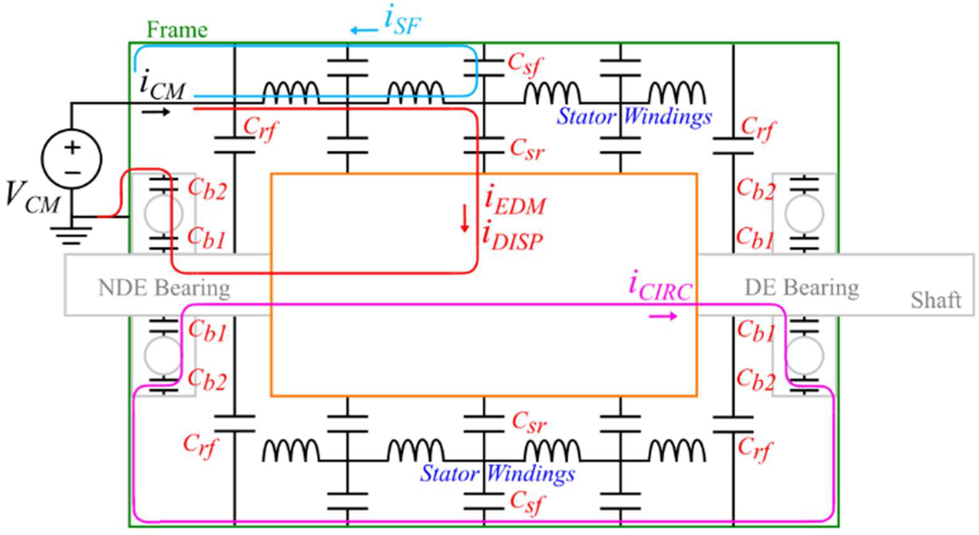
2.1. Displacement Current

The bearing displacement current i_DISP (see Figure 1) is due to the time rate of change of the shaft voltage, which acts across the inner and outer race of both the drive end (DE) and non-drive end (NDE) bearings. This mode of bearing current is small in amplitude, and researchers agree that bearing displacement current has negligible effects on bearing operation and lifetime [6,29].

2.2. Stator-to-Frame Current and Circulating Bearing Current

The stator-to-frame current i_SF (see Figure 1) is the largest component of the CM current, due to the large capacitive coupling C_SF between the stator windings and stator core, where the core is electrically connected to the frame of the machine, which is at system ground potential. The flux generated from this mode of CM current magnetically couples to the loop that comprises the rotor, DE bearing, frame, and NDE bearing. When the high frequency induced voltage exceeds the dielectric strength of the bearing lubricant, a circulating bearing current i_CIRC is produced on this path, as shown in Figure 1 [30].

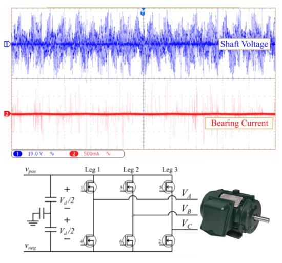
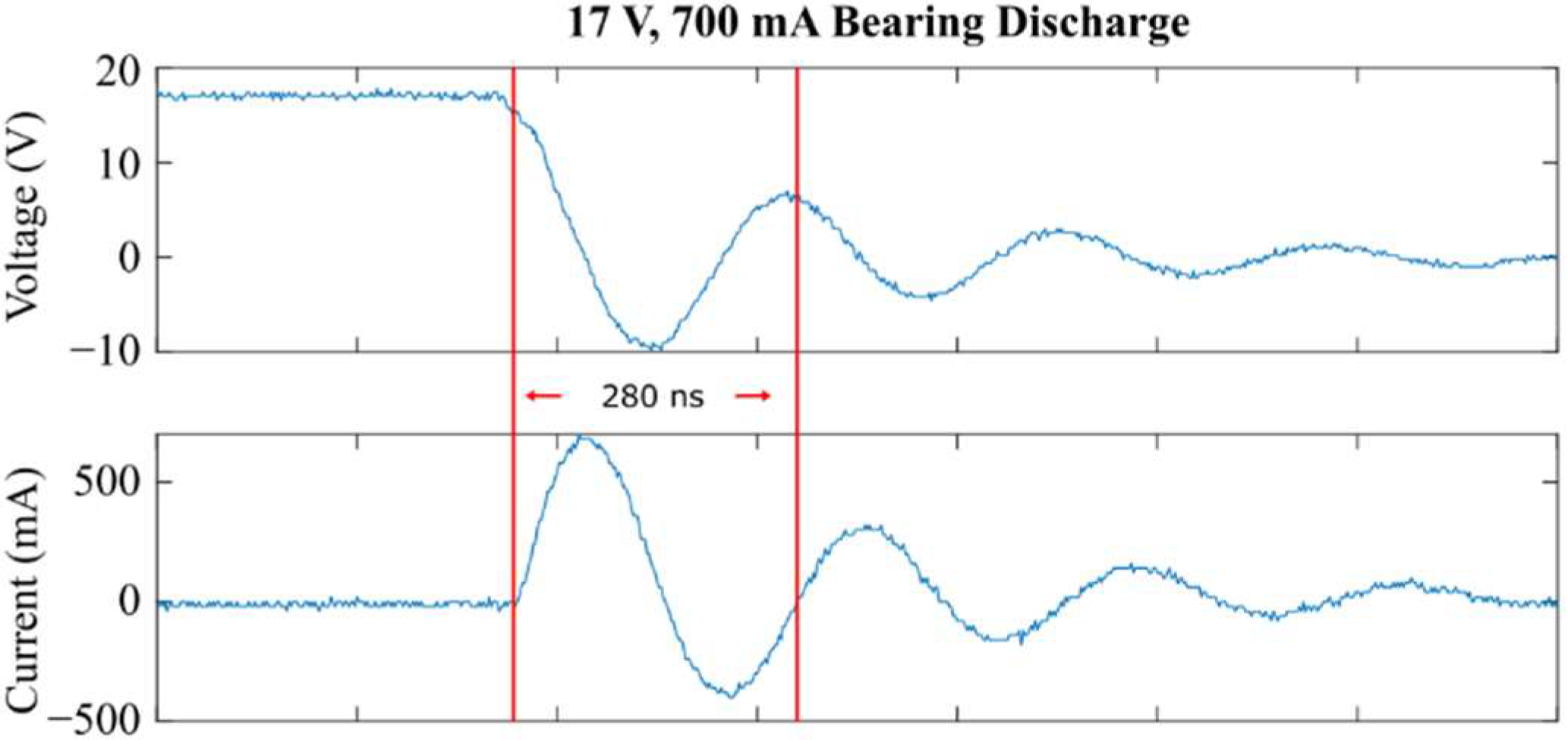
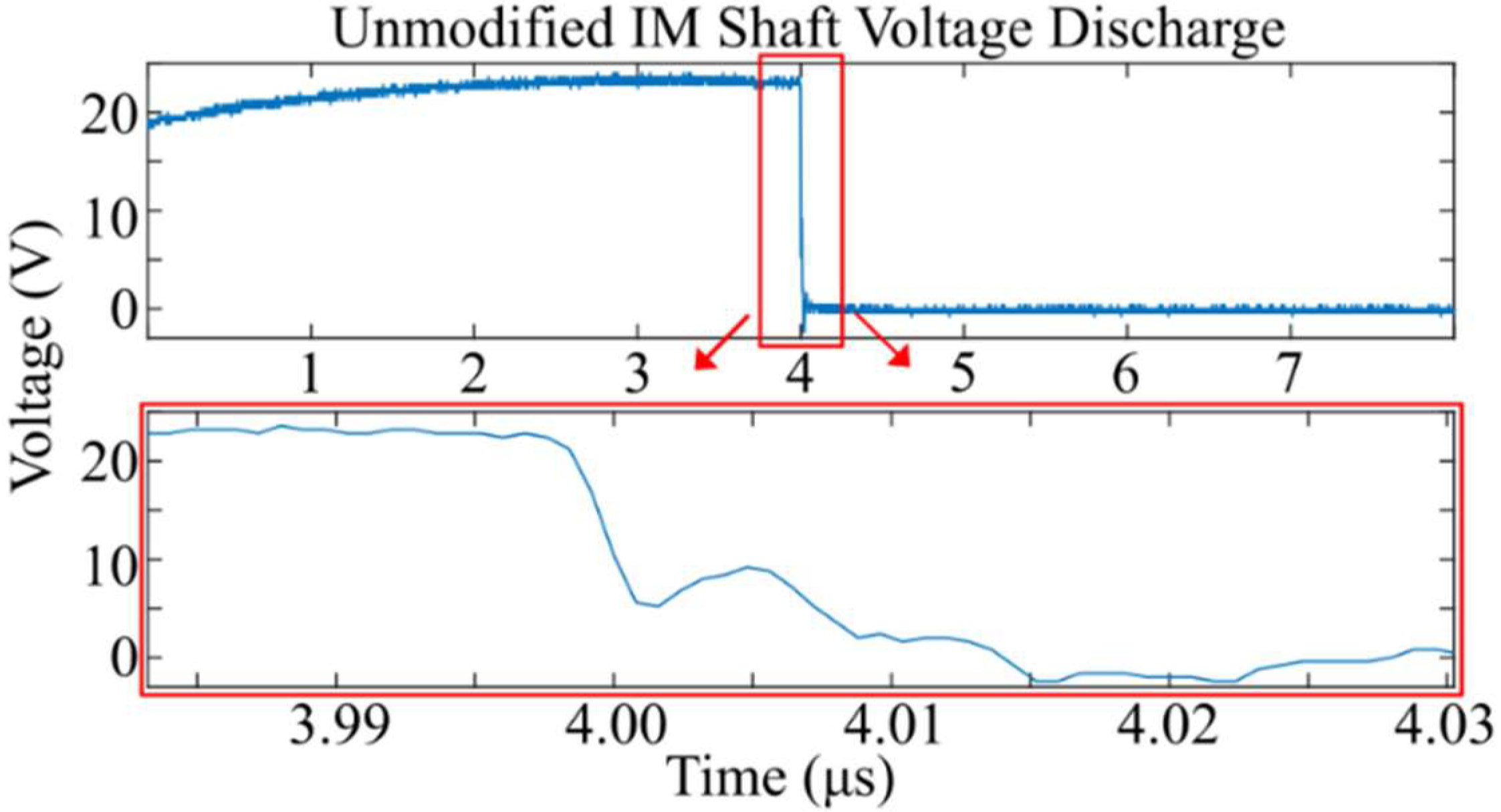
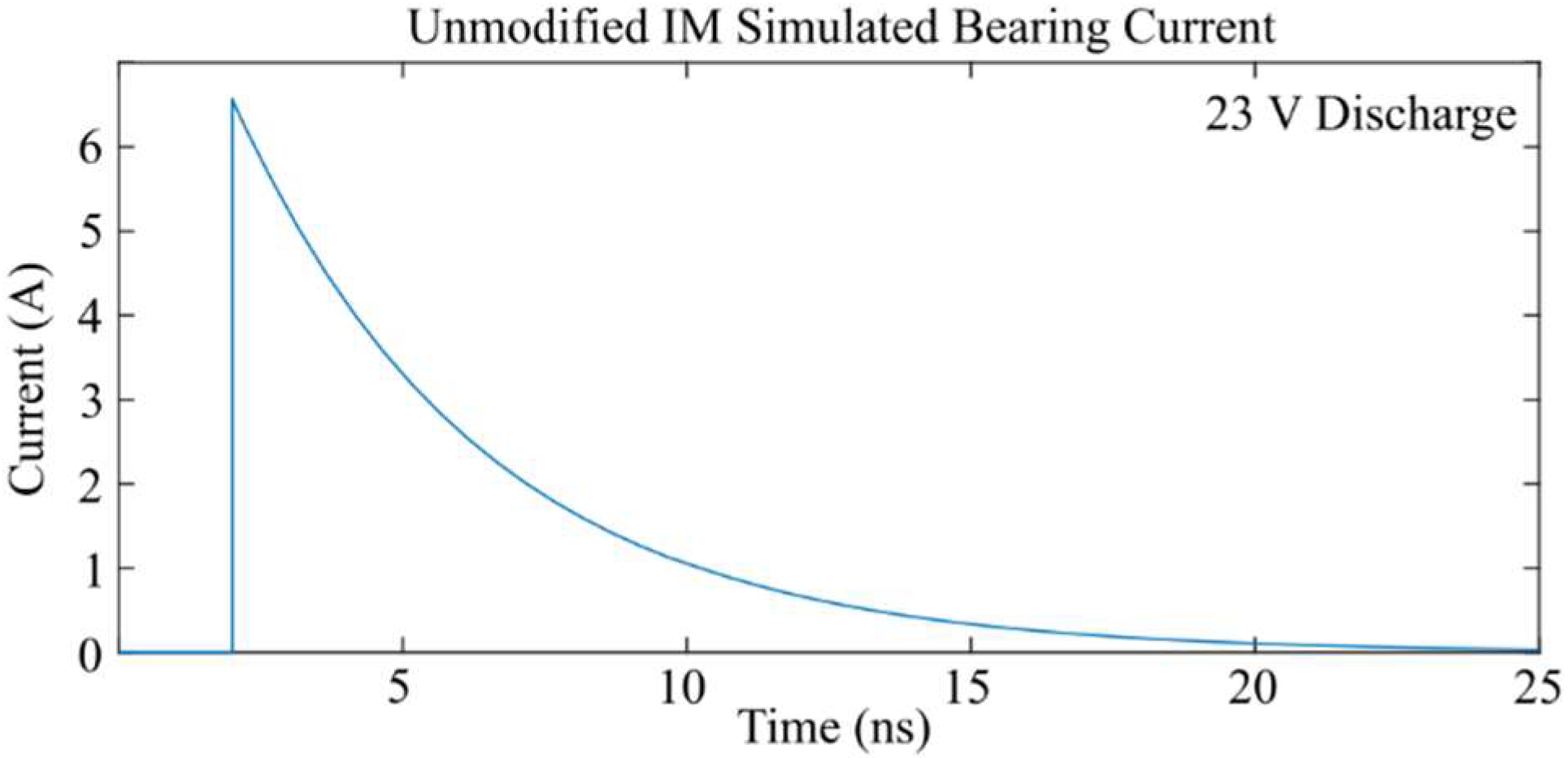
2.3. Electric Discharge Machining Bearing Current

During a rising or falling edge of the CM voltage, a voltage is produced on the shaft of the machine via electrostatic (capacitive) coupling, according to Equation (2). As the machine spins, the bearing lubricant forms a thin film on which bearing rolling elements ride, achieving hydrodynamic lubrication. An electric field is formed across the thin bearing lubricant film due to the shaft voltage, creating a bearing capacitance C_b. Two separate capacitances are formed between the inner race to ball and ball to outer race, although they are often lumped together into a single component. When the shaft voltage produces an electric field that exceeds the dielectric strength of the lubricant film, the lubricant breaks down resulting in an electric discharge machining bearing current i_EDM (see Figure 1), where all the electrostatic energy stored in the rotor assembly capacitances is dissipated during the discharge. Since the ratio of energy dissipated to bearing ball/race discharge surface area is large, the temperature increases significantly, and local melting may occur at the bearing steel if the temperature exceeds the solidus temperature of the bearing steel.

The damaging EDM discharges produce pits and pillars on the ball and race surfaces on a microscopic level, which appear as frosting and fluting on a macroscopic level. Over time, these EDM bearing currents result in premature bearing failure due to increased vibration. EDM damage can be seen on the outer race of Figure 3. This mode of bearing damage is much faster than metal fatigue bearing damage, and significantly reduces operational lifetime [31]. This is the form of bearing current that will be considered in this paper.

Studies on the effect of voltage rise time on dielectric breakdown voltage indicate that a faster rise time causes an ionization shock to the dielectric [32,33,34,35,36], which allows the voltage to reach a higher value before breakdown than it otherwise would for a slower rise time. This pulsed dielectric (PD) theory explains, for example, the increase in shaft voltage for Si PWM inverters when compared to the same machine driven by line voltages [7]. Since wide bandgap devices have even faster voltage rise times, it is expected that shaft voltage and EDM bearing current amplitudes will increase further, posing a significant threat to bearing health. In this paper, experimental data will be used to explain how the BVR theory and pulsed dielectric theory can be synthesized. According to the BVR theory, the shaft voltage is a function of a capacitive voltage divider. On the other hand, the pulsed dielectric theory states that the breakdown voltage of the shaft is dependent on the device slew rate. Therefore, further clarification is required to understand how these theories describe the EDM phenomenon.

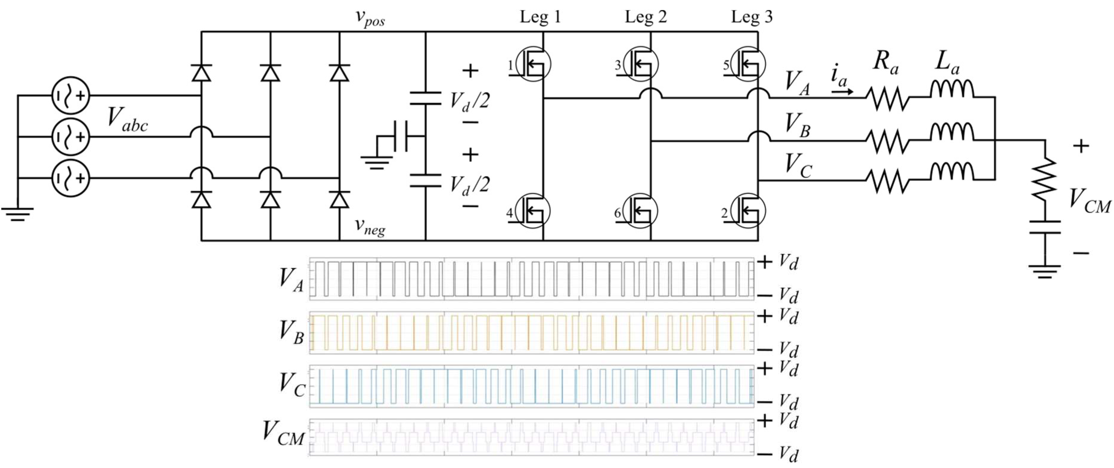
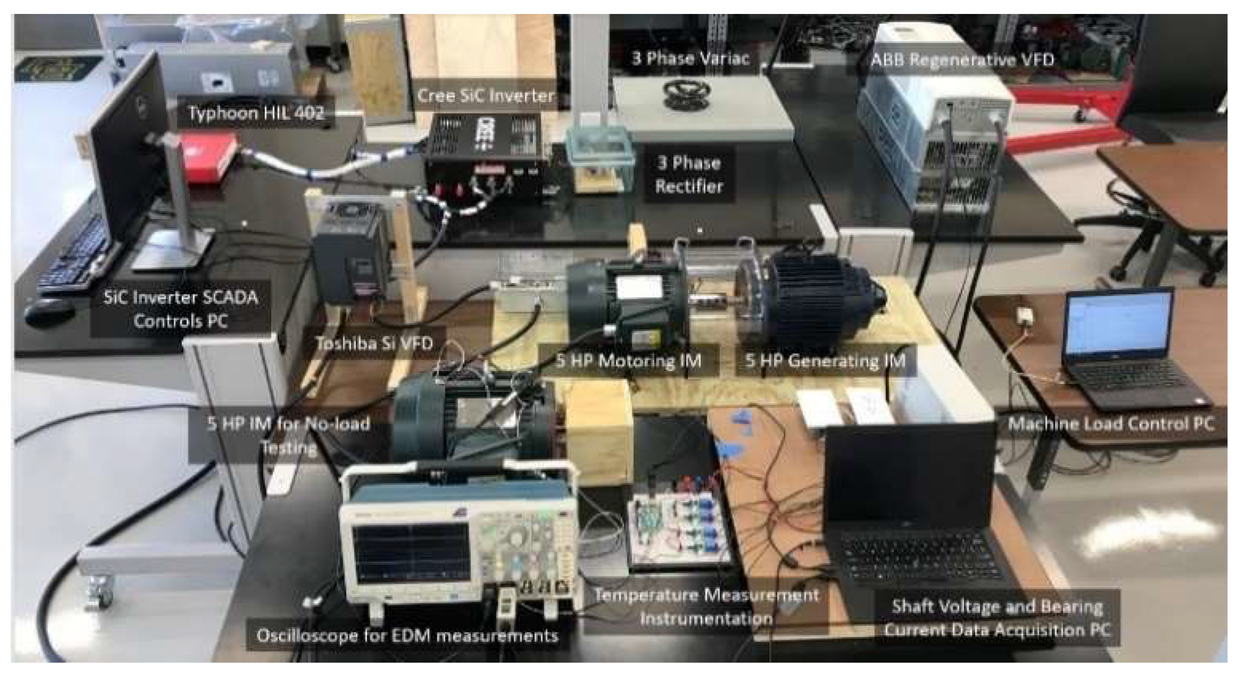
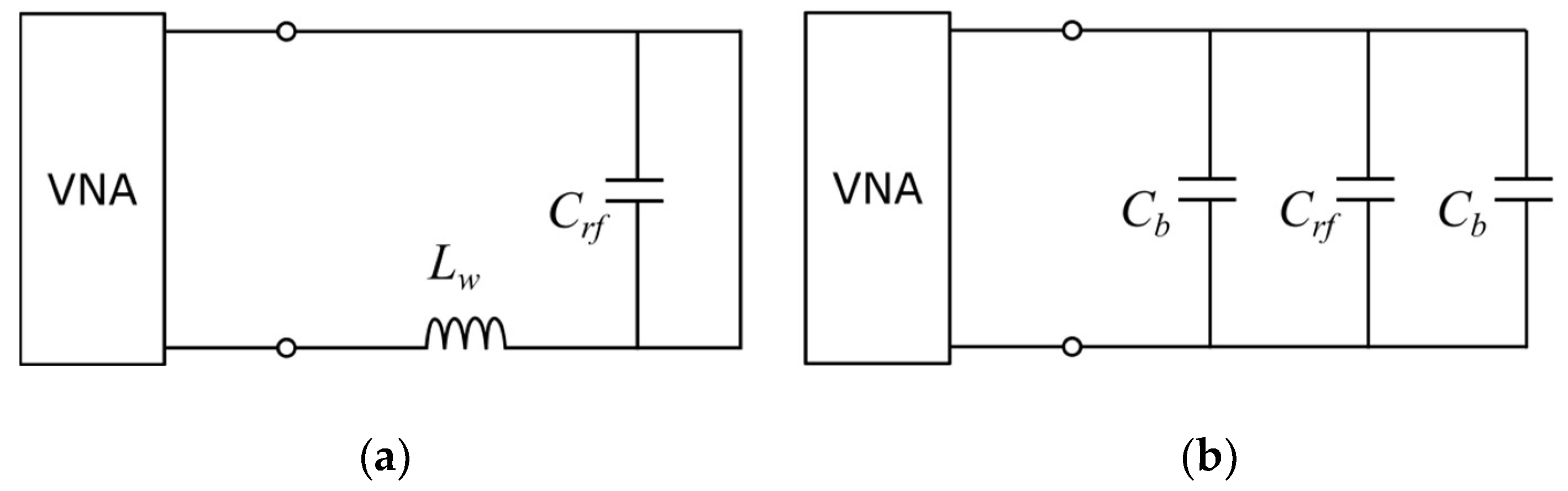
3. Materials and Methods

To allow for experimental measurements of EDM bearing currents, an IM was modified by installing polyoxymethylene insulating sleeves into the frame of the motor for both the DE and NDE bearings to sit in, which isolates the bearing outer races from the frame of the machine. A jumper wire is then attached from the outer race of each bearing to the frame of the machine, forcing the EDM current path through the wire [23].

It should be noted that although a measurement is now available, it is impossible to directly measure the actual bearing current [6], and the measurement modification alters the discharge phenomenon. As can be seen in Figure 4, the insulating sleeves introduce an isolation capacitance C_i, while the jumper wire for bearing current measurement introduces a parasitic inductance L_w, parasitics which are not negligible at EDM bearing current discharge frequencies. However, even though the modification has altered the true measurement, the apparent bearing current measurement is still proportional to the actual value [6]. For this reason, this paper will refer to experimentally measured bearing current as “apparent bearing current”. The equivalent circuit model for the EDM bearing current phenomenon is shown in Figure 4. The discharge resistance is denoted R_b. The actual bearing current for the modified machine can be computed by obtaining precise values for the components of Figure 4 (C_i, L_w, C_b, R_b). Discharge modeling considerations will be discussed in Section 4. The bearing discharge is modeled with a simple RC circuit and switch [37], and the parasitic components from the motor modification are included.

During an EDM discharge, the switch on either the DE or NDE bearing of Figure 4 is closed, allowing the electrostatic energy stored in the shaft to be released through the bearing. The parasitic components of Figure 4 cause the measured shaft voltages and bearing currents to appear as damped sinusoids, as can be seen in Figure 5.

Although an EDM event occurs at just one bearing, the bearing capacitance of the opposite bearing is included in the parasitics that cause the ringing discharge phenomenon, therefore a discharge at one bearing can be seen in the measurement wire inductance of the other bearing [22], although with a much smaller amplitude. It is important to distinguish these EDM bearing currents from circulating bearing currents, even though like circulating bearing currents an EDM discharge can be seen at the opposite bearing from where it occurred. For circulating bearing currents, the current magnitude is equal and opposite at each bearing, as each bearing dielectric film has been punctured, where only one bearing dielectric film is punctured for EDM bearing currents. In this paper, the breakdown voltage and the peak of the bearing current are used to characterize each discharge that occurs. For example, the EDM discharge of Figure 5 is characterized as a 17 V, 700 mA discharge.

The experimental testbed employed to obtain shaft voltage and bearing current data is shown in Figure 6. In this testbed, two two-level six-switch inverters, namely a Toshiba VF-S15 Si-based VFD (2800 V/µs) and a Cree SiC inverter evaluation unit (11,500 V/µs) [26] are used to drive a 460 V, 4 pole, 1800 rpm, 5 hp squirrel cage IM. To enable acquisition of high resolution data for late modelling, the data shown in Figure 5 was collected using a scope sampling rate of 1.25 GHz (Record Length 1000, 80 ns/div, 10 div).

The design of the SiC motor drive system is detailed in [38]. The IM is coupled to another IM to provide loading, using an insulated shaft coupling to prevent bearing currents from discharging in one machine due to shaft voltages produced in the other. An ABB regenerative VFD is used as a part of the dynamometer system to apply torque commands to the load machine. In addition to the motor modifications mentioned in the previous section, a thermistor was placed on the bearings to monitor bearing temperature. To prevent the circulating bearing current phenomenon from occurring, measurements were carried out only at the DE wire, leaving the opposite end disconnected. The IM has a BVR of 8% (a CM voltage transient of 426 V produced a 33 V shaft voltage) and employs SKF 6306-2Z/C3GJN bearings. A Tektronix MDO3014 oscilloscope and TCP0030A current probe was used to measure the apparent bearing current through the DE bearing. It was found that in order to optimize the ability to accurately measure the magnitude of the less frequent, but more damaging, of the large current discharges, a lower sensitivity combination on the current probe was useful. This did result in coarsening of the data and, indeed, missing many low amplitude discharges. Because these low energy discharges have negligible impact on the bearing surface, neglecting these discharges does not affect subsequent statistical evaluation of bearing lifetimes. In addition, a TPP0250 voltage probe and graphite brush were used to collect shaft voltage waveform data.

For the data collection, a 50 MHz sampling frequency was implemented on the scope to accurately capture the high frequency oscillations of the shaft voltage and EDM bearing currents, which discharged at ~10 MHz. We found that increasing the sampling rate didn’t improve peak amplitude results, and significantly limited the number of discharges that could be captured, decreasing the quality of the sampling statistics used in the evaluation of the probability density functions describing the discharge frequencies. To provide high quality counting statistics, 5 replicates of the data were collected at each bearing temperature to yield a complete data set.

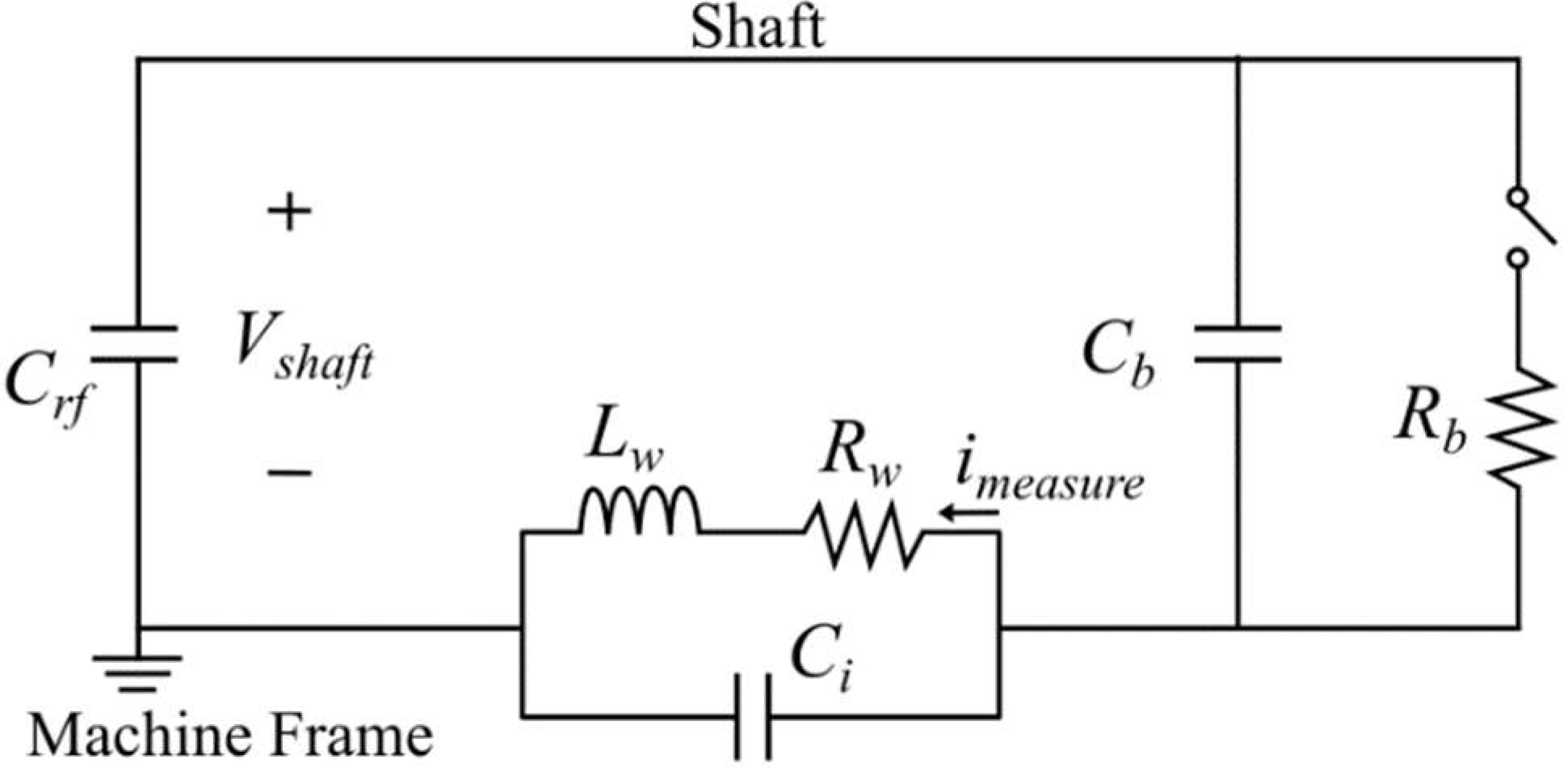
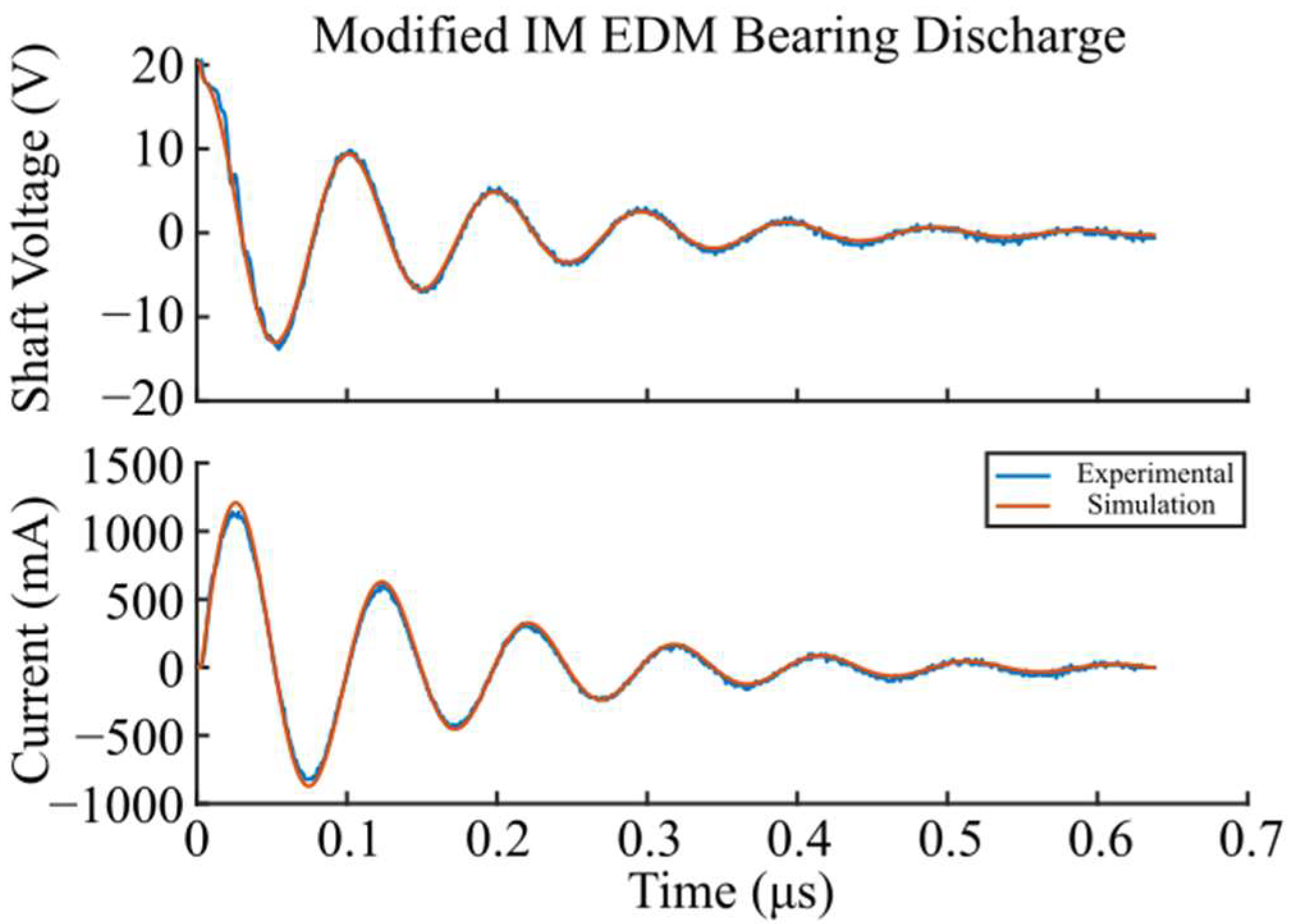
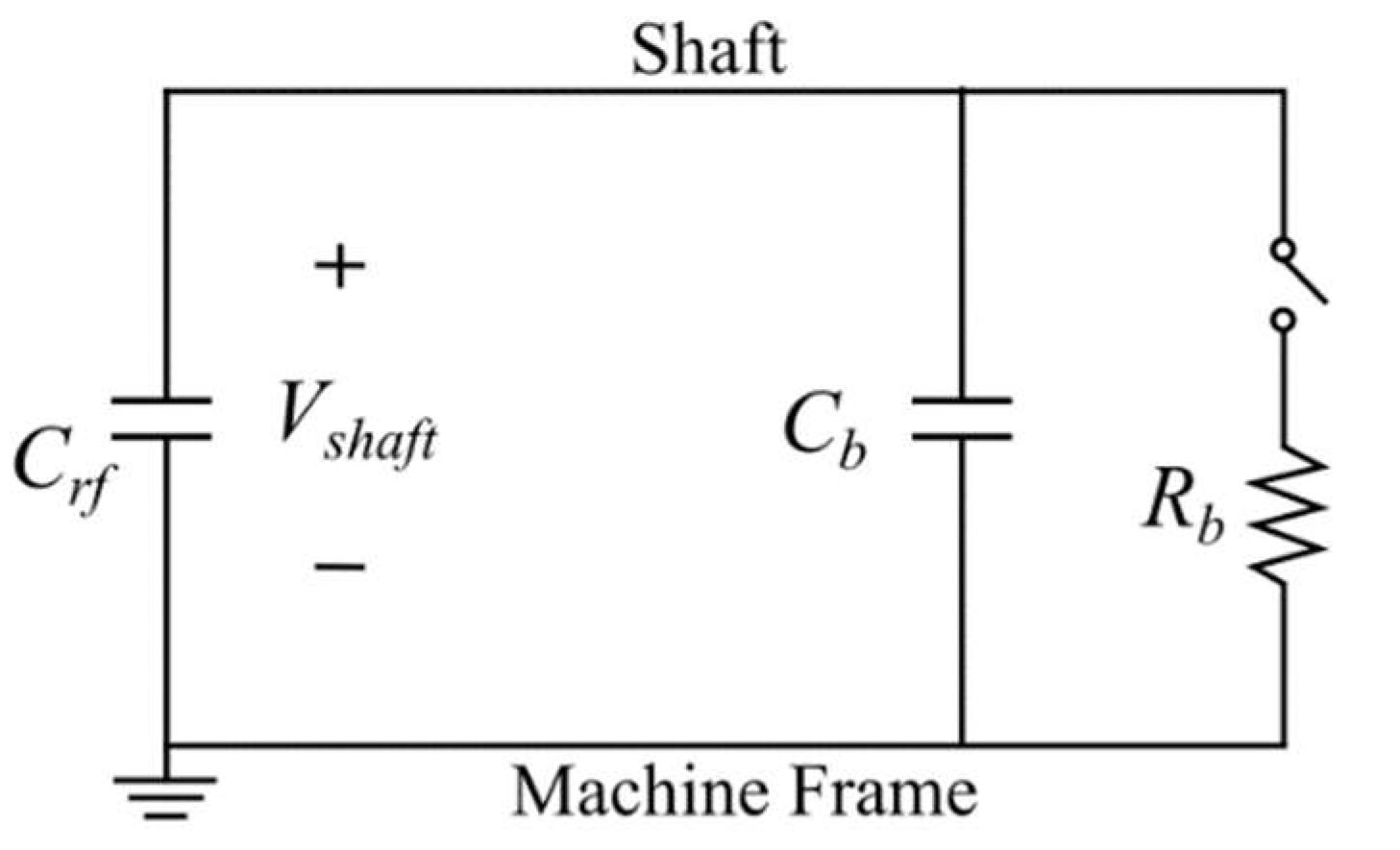
4. EDM Bearing Current Modeling

This section details circuit models developed in PSpice that model the behavior of the EDM discharges for both modified and unmodified IMs.

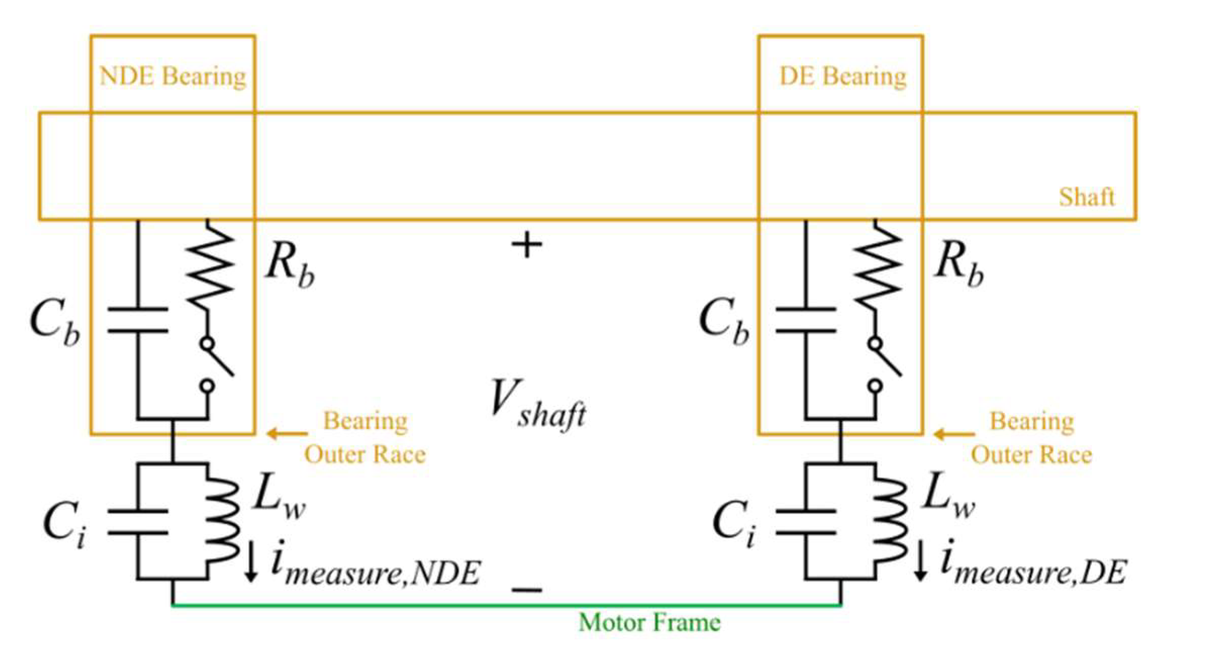
4.1. Modified Induction Motor

The equivalent circuit model for analyzing EDM discharge transients at the DE bearing is shown in Figure 7. Network analyzer S₁₁ parameters were used to extract the component values for C_rf, C_i, and L_w under rated speed and zero speed conditions using a NanoVNA vector network analyzer. At rated speed and low bearing operational temperatures, the bearing lubricant remains intact allowing for a network analyzer measurement of the parallel combination of C_rf and the two bearing capacitances at the DE and NDE. The rated speed test was performed on an unmodified IM, which ensured that the measurement circuitry did not alter the measurement. At zero speed, the bearing lubricant film is thin enough to conduct due to direct contact of the bearing ball and race surfaces, resulting in a short across C_b, which in turn allows for a network analyzer measurement of L_w. For C_i, this parameter was extracted by removing the motor end and measuring the S₁₁ parameters between the bearing outer race and the machine frame. An additional parallel plate capacitor calculation using a polyoxymethylene dielectric was performed for C_i. The bearing capacitance C_b was also characterized on a separate testbed using S₁₁ parameters. Additionally, a function generator with 50 Ω source resistance was utilized to apply a voltage step to the machine shaft. Since the equivalent circuit of the voltage step is a first order RC circuit at rated speed (lubricant remains intact), the charging rate can be used to extract the net capacitance on the shaft, which then can be used to produce a C_rf measurement. It was determined that the grounding wire resistance R_w is negligible compared to the discharge resistance R_b, and that the isolation capacitance has negligible effects on the discharge transient. Finally, as was available, the measured circuit component values were compared with values published in the literature as a final check. In Figure 8, the equivalent circuit models for zero speed and rated speed conditions are provided.

The EDM discharge model of Figure 7 was implemented in PSpice. Parameter tuning was performed using the PSpice Optimizer tool. This tool tunes the parameters of the simulation model to match experimental shaft voltage and bearing current measurements. Experimentally measured and literature values were used as seeds for the refined parameters, and the model refinement was approached by refining parameters in different order combinations, to ensure the quality of the results.

Table 1. Summary of modified IM circuit modeling component values with final values in the “PSpice Optimizer” row.

Component	Lw	Rb	Ci	Crf	Cb
Literature	-	1–20 Ω [6]	-	-	0.2–1 nF [39]
Calculation	-	-	141 pF	-	-
Network Analyzer	300 nH	-	97 pF	1826 pF	199 pF
Step Response	-	-	-	1500 pF	-
PSpice Optimizer	213 nH	1–20 Ω	120 pF	1045 pF	200 pF

summarizes the modified IM circuit modeling component values, and Figure 9 shows experimental and simulation results for a 20 V, 1150 mA discharge.

From Figure 9, the PSpice simulation model accurately describes the EDM discharge phenomenon. For this 20 V, 1150 mA discharge, a bearing resistance of R_b = 3.25 Ω optimized the fit, although while fitting various discharges it was determined that the bearing discharge resistance varies from 1–20 Ω, as confirmed in [6]. This can be explained by the variable nature of the discharge gap distance within the bearing.

4.2. Modified Induction Motor

The PSpice model developed from the previous section can be used to extract the EDM bearing current profile and amplitude for an unmodified IM where a bearing current measurement is not available. In Figure 10, a 23 V shaft voltage discharge that occurs on an unmodified IM is shown.

Since the grounding wire is now no longer included in the discharge circuitry, the second order oscillatory effects are also removed from the discharge, and the discharge takes ~17 ns to completely dissipate to 0 V, compared to the discharge of the modified IM (Figure 9) which takes ~600 ns to completely dissipate to 0 V. The equivalent circuit model for the unmodified IM is shown in Figure 11.

With the isolation capacitance and jumper wire removed from the system, the discharge behaves as a first order RC circuit. The same parameters as shown in Table 1 are utilized, and the resulting EDM bearing current is shown in Figure 12. Here again, a bearing resistance of R_b = 3.5 Ω allows the shaft voltage to completely discharge within ~17 ns. Since the discharge models of Figure 7 and Figure 11 are linear systems, the ratio between the peak current for a modified and unmodified IM are the same for various shaft discharge voltages, which for the measurements in this research is:

$$\phi =\frac{{\widehat{I}}_{MOD}}{{\widehat{I}}_{UNMOD}}=0.2$$

(3)

This ratio is dependent on the inductance of the jumper wire L_w. As L_w → 0, the bearing current amplitude approaches ${\widehat{I}}_{UNMOD}$.

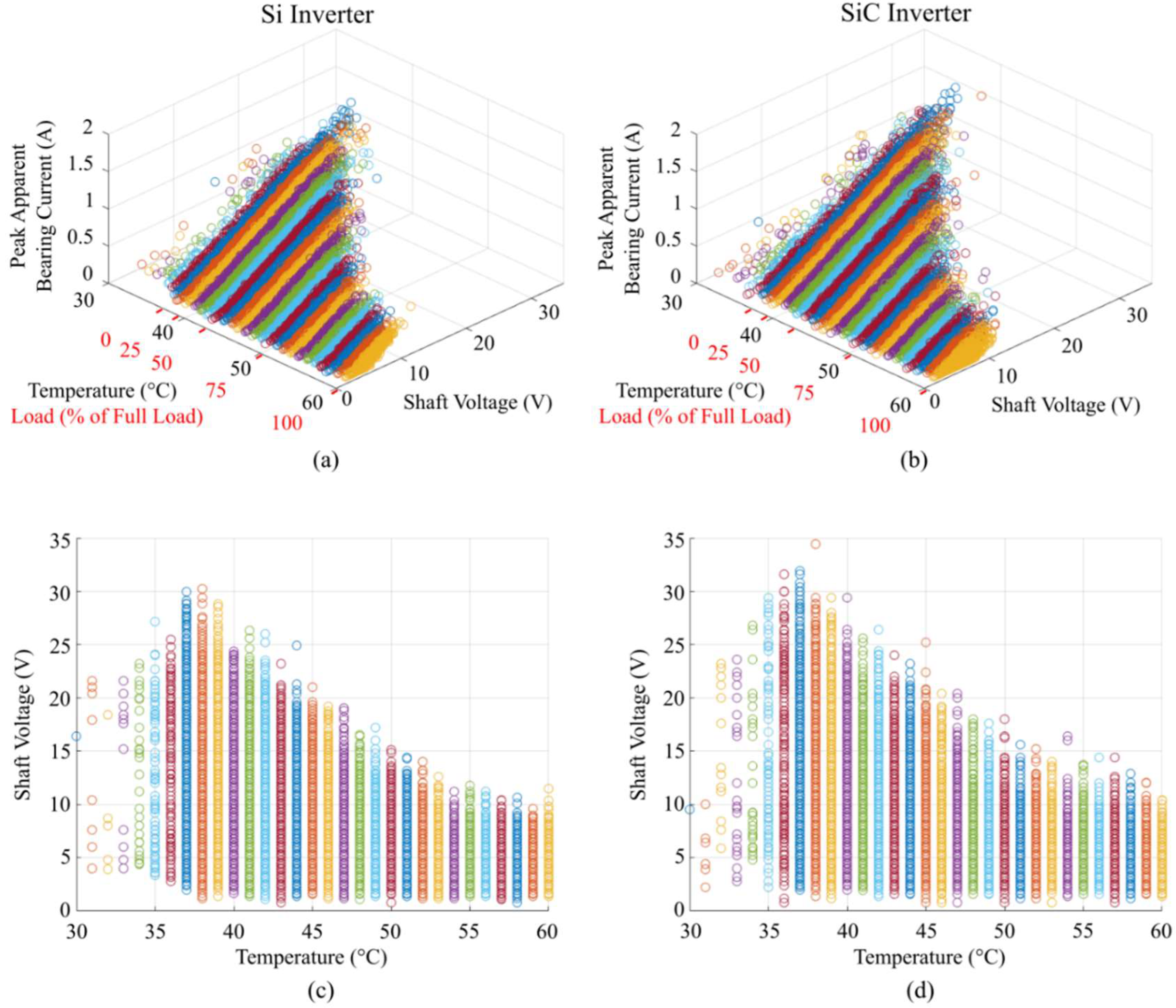
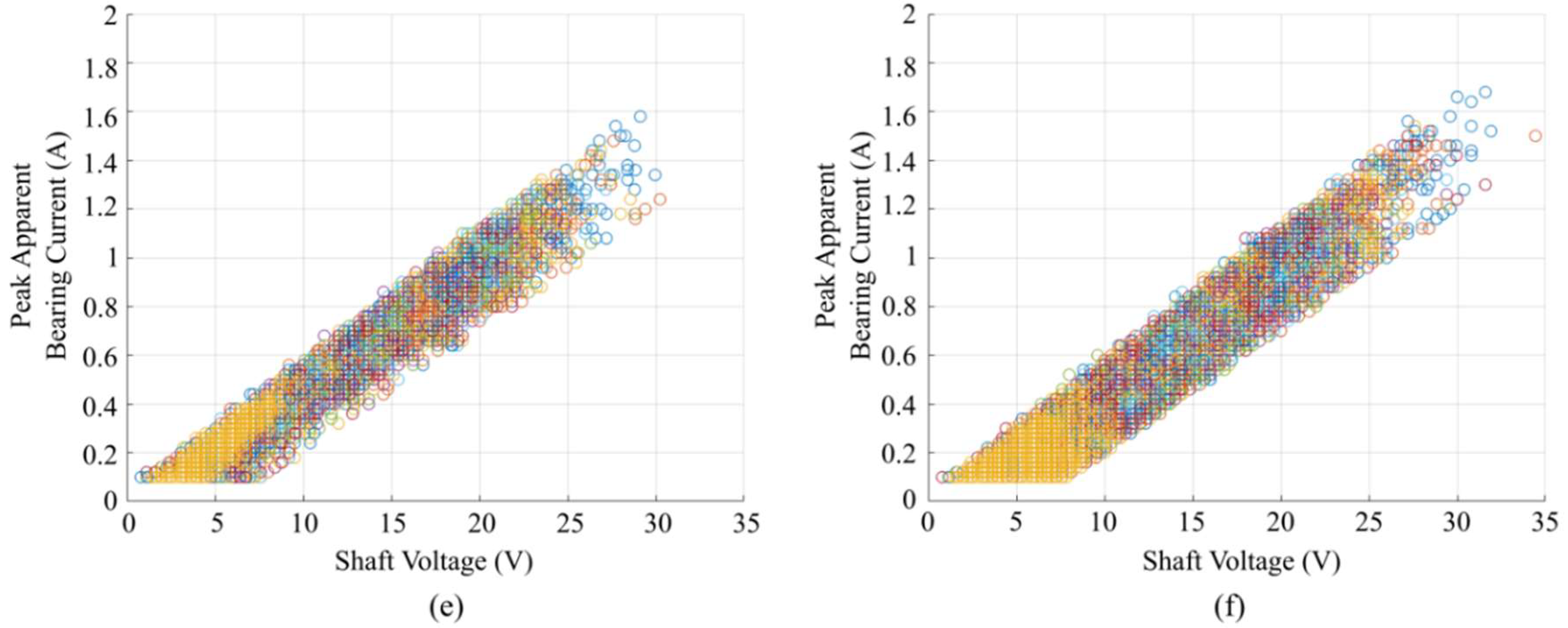
5. Shaft Voltages and EDM Bearing Currents Due to Si and SiC Inverters

To investigate the impact of SiC inverter switching speeds on machine bearing EDM currents relative to Si inverters, an experimental procedure was developed for the testbed of Figure 6. The bearings operate in a temperature range between ambient (~20 °C) and full machine loading (~60 °C). At various operating points between 30–60 °C, 1000 ms of shaft voltage and EDM bearing current data were recorded on the modified IM. Once the data was collected, an algorithm was developed that iterates through each waveform and extracts the peak apparent bearing current, as well as the shaft breakdown voltage that produced the bearing discharge. Only discharges with an amplitude greater than 50 mA were recorded to prevent current probe noise due to bearing displacement current from affecting the data. Additionally, discharges less than 50 mA most likely do not cause EDM damage to the race surface, and therefore do not affect bearing operational lifetime. Therefore, these small amplitude discharges can be disregarded. The results from this experimental procedure are shown in Figure 13, where all the extracted data is displayed. All data was collected at a motor speed of 1800 rpm, a switching frequency of 10 kHz, and an ambient temperature of 20 °C. Each data point of Figure 13 denotes a discharge event, where the shaft breakdown voltage and peak apparent bearing current are defined as shown in Figure 5.

As the bearing temperature and machine load increase, the maximum amplitude of the shaft voltage and bearing current discharges decrease, due to a thinner lubricant film at higher temperatures. A thinner lubricant leads to an increase in the electric field between the inner and outer race of the bearing for the same shaft voltage, which results in discharges occurring at lower voltages. In other words, the maximum possible shaft voltage for each operating point decreases with an increase in temperature and load because the lubricant dielectric cannot support an electric field greater than the electric field required to produce dielectric breakdown and a discharge. At a 37 °C bearing operational temperature, the lubricant film is just becoming thin enough to produce discharges. Since this is the operational point with the thickest lubricant film where discharges are present, it is also the operating point with the largest amplitude of shaft voltages and bearing currents, which are the most damaging. Below 37 °C, the lubricant film is thick enough that a discharge event becomes very rare (34 discharge events at 34 °C in 1000 ms vs. 10,961 discharge events at 39 °C in 1000 ms), and the shaft voltage is a fraction of the machine CM voltage.

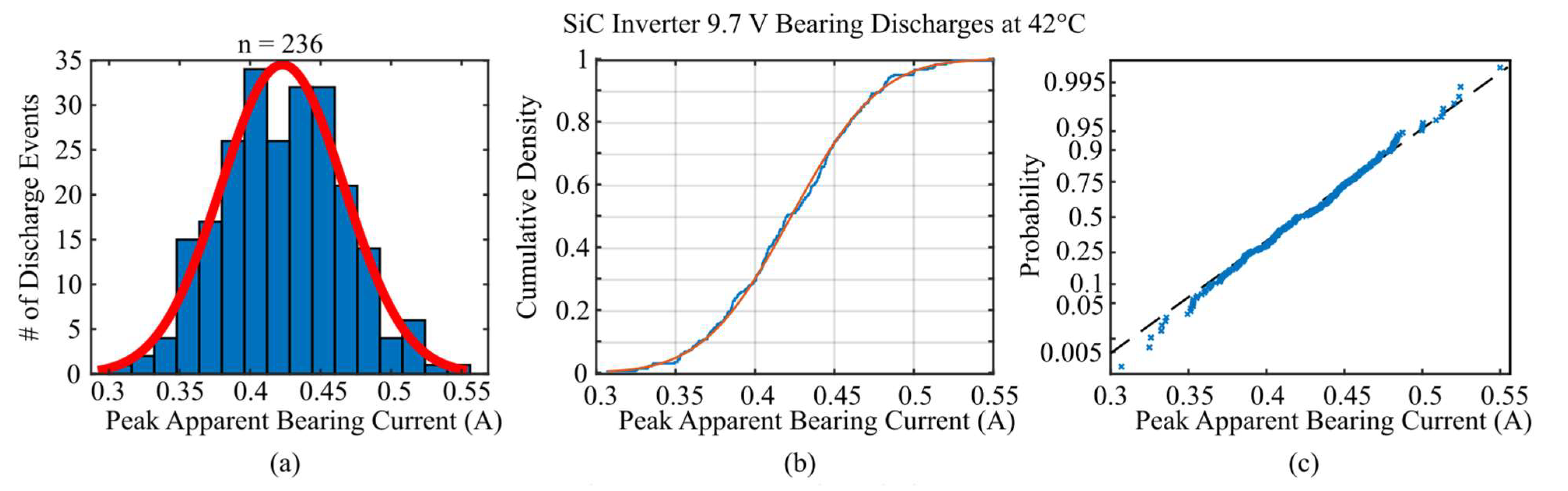
5.1. Peak Apparent Bearing Current Distribution

The peak apparent bearing current amplitude is linearly dependent on the shaft breakdown voltage at each motor operational point due to the linearity of the discharge circuit (Section 3, Figure 13e,d). A line of best fit was calculated using a least squares fit for the data displayed in Figure 13e,d.

$$i_{fit}\left(v\right)=0.05v-0.07, i_{fit}>0$$

(4)

While this least squares line fits the data shown, inspection of Figure 13e,d reveals that the apparent bearing current for any amplitude of shaft voltage has a distribution about the value given by Equation (4), as shown in Figure 14. This is due to the variable discharge resistance. To investigate this, three different discharge sets were analyzed for the Si and SiC inverter shaft voltage and bearing current data: 9.7 V discharges produced by the SiC inverter at 42 °C, 7 V discharges produced by the SiC inverter at 37 °C, and 15 V discharges created by the Si inverter at 38 °C. It was determined that the peak apparent bearing current for any particular shaft voltage follows a normal distribution, the results of which can be seen graphically in Figure 14 for the SiC inverter 9.7 V discharges at 42 °C.

From Figure 14, the plots demonstrate the normally distributed peak apparent bearing current data for any particular shaft breakdown voltage. A few modifications to the data were necessary. First, small groups of outliers were identified beyond three standard deviations below the mean of each distribution. These outliers are due to algorithm error. The algorithm used to extract discharge amplitudes iterates through the shaft voltage and apparent bearing current oscilloscope waveforms, searching for local maxima in the bearing current signal. When a bearing current local maximum is detected, it is recorded along with the maximum shaft voltage within that local area. Although effective, the algorithm is prone to occasional error such as noise and larger amplitude displacement currents. These outliers were thoroughly investigated, and it was determined from viewing the shaft voltage and bearing current waveforms that discharge events recorded below three standard deviations from the peak apparent bearing current mean were false readings from the algorithm, and therefore can be disregarded. Second, the ADC resolution of the Tektronix MDO3014 oscilloscope used in this application was 20 mA, therefore each data point extracted by the algorithm falls into a bin with 20 mA spacing. In order to test for normality of the data, the Shapiro-Wilk Test was implemented [40], which was used in tandem with visual evaluations of Figure 14. The Shapiro-Wilk Test is very sensitive to discrete data. By adding a uniformly distributed random noise signal to the data with an amplitude of 0.02, the data can be moved out of the discrete bins into a continuous distribution without altering the mean or standard deviation of the distribution. To see the effects of the injected noise and elimination of the outliers that are a result of algorithm error, a probability plot of the raw, unmodified data is provided in Figure 15. This plot does not contain the uniformly distributed noise and includes the erroneous outliers.

Visual comparison of Figure 15 and Figure 14c demonstrates how the outliers due to algorithm error do not follow the main body of data that is normally distributed, and cause the tail of the distribution on the upper end (>0.5 A) to begin departing from the theoretical normal distribution line. Additionally, the discrete data bins spaced 20 mA apart are also apparent. Discarding the irrelevant outliers and adding the uniformly distributed noise allowed for accurate use of the Shapiro-Wilk test and for ease in visually evaluating the cumulative density and probability plots of each distribution. The numerical results of the data displayed graphically in Figure 14 are shown in

Table 2. Normal distribution statistics for peak apparent bearing current at various shaft discharge voltages for the Si and SiC inverter.

Inverter		SiC	SiC	Si
Bearing Temperature (°C)		42	37	38
Shaft Voltage (V)		9.7	7	15
ifit (A) (Equation (4))		0.415	0.280	0.680
Peak Apparent Bearing Current (A)	µ	0.423	0.272	0.701
	δ (Equation (5))	1.9%	−2.9%	3.1%
	σ	0.044	0.035	0.059
Shapiro Wilk Test (α = 0.05)		accept	accept	accept

, along with the other two shaft voltage conditions previously mentioned. A Shapiro-Wilk Test for normality was conducted for each case at a significance level of α = 0.05. A percent error statistic is also calculated to compare the mean value µ of the current distribution with the fitted line of Equation (4). The normal distribution standard deviation is denoted σ.

$$\delta =\frac{i_{\mu }-i_{fit}}{i_{fit}}\times 100\%$$

(5)

From Table 2, the Shapiro Wilk null hypothesis to determine if a normal distribution is a reasonable assumption of the peak bearing current distributions for a single shaft voltage can be accepted with 95% probability (α = 0.05). The primary reason for the current distribution is the varying bearing discharge resistance between each discharge. This can be attributed to slight variations in lubricant thickness upon breakdown for each discharge, asperity differences on the race and ball surfaces, alignment of the bearing and shaft, and radial and axial bearing loads. Therefore, the potential discharge resistances of each discharge also follow a normal distribution.

5.2. Discharge Resistance Distribution

To investigate the discharge resistance distributions, the modified IM equivalent circuit discharge model of Section 3 was employed to explore the bearing discharge resistances that are associated with the peak apparent bearing current amplitudes measured that form the distributions of Table 2. A parameter sweep was performed in PSpice on the bearing discharge resistance, resulting in varying peak apparent bearing current amplitudes. The results can be seen in Figure 16 for the 9.7 V SiC discharges at 42 °C.

Markers are provided to demonstrate how the mean and standard deviation of the current distributions align with the mean and standard deviation of the bearing discharge resistance distributions. A summary of the bearing discharge resistance normal distributions is provided in

Table 3. Summary of bearing discharge resistance normal distributions produced by the SiC inverter at 9.7 V, 42 °C, and 7 V, 37 °C, and for the Si inverter at 15 V, 38 °C.

Inverter		SiC	SiC	Si
Bearing Temperature (°C)		42	37	38
Shaft Voltage (V)		9.7	7	15
Bearing Discharge Resistance (Ω)	µ	11.9	16.5	9.0
	σ	3.4	4.8	2.3

. In the literature, bearing discharge resistances are reported in the range of 1–20 Ω [6]. The results displayed in Table 3 validate the bearing discharge resistance value.

5.3. Discharge Amplitude

This section analyzes the parameters that affect the amplitudes of the EDM discharges. To compare the change in maximum discharge amplitude at each operational temperature, an average of the 100 largest discharges at each temperature point are compared between Si and SiC inverters, and the shaft voltage for a line-driven machine is also recorded to provide a reference. The increase in shaft discharge voltage between SiC and Si inverters was calculated as:

$$\%\Delta =\frac{V_{SiC}-V_{Si}}{V_{Si}}\times 100\%$$

(6)

The corresponding discharge energies were also calculated using the models of Section 3:

$$E_{discharge}=\frac{1}{2}\left(C_{rf}+2C_b\right)V_{shaft}{}^2$$

(7)

Both the Si and SiC inverter started to experience shaft voltage breakdown and EDM bearing current shoot through at a bearing temperature of ~37 °C, while the line driven machine shaft voltage begins to break down at ~51 °C. The results can be seen in Figure 17, where the result of Equation (6) is also plotted.

On average when comparing Si and SiC devices, the largest shaft voltage discharges increased by 8.2% across all temperatures, and since the resulting peak bearing current is linearly proportional to the shaft breakdown voltage, the bearing current amplitude increases as well. The results show that dielectric breakdown theory due to device rise time becomes especially relevant above bearing temperatures of 50 °C (machine loads >75% of rated load), as the SiC shaft voltage showed an average increase of 12.7% in this region compared to Si.

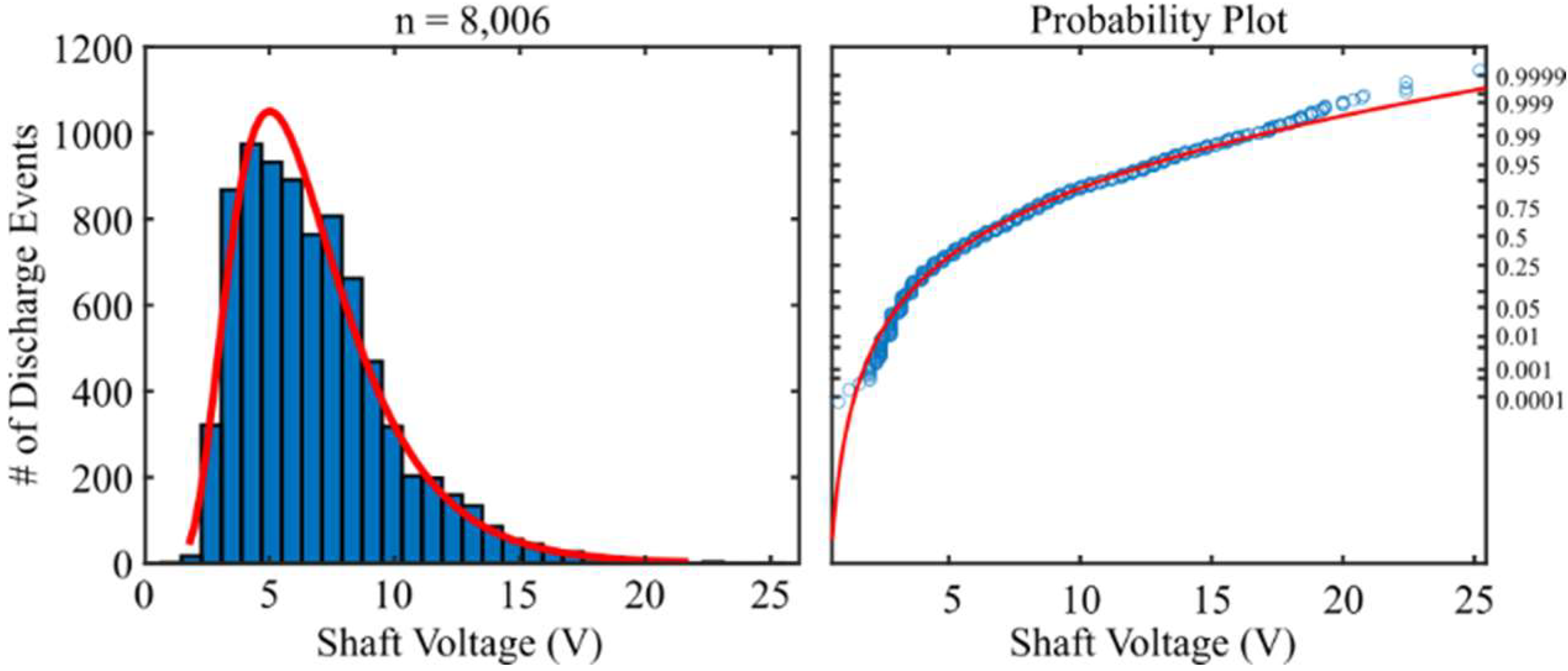
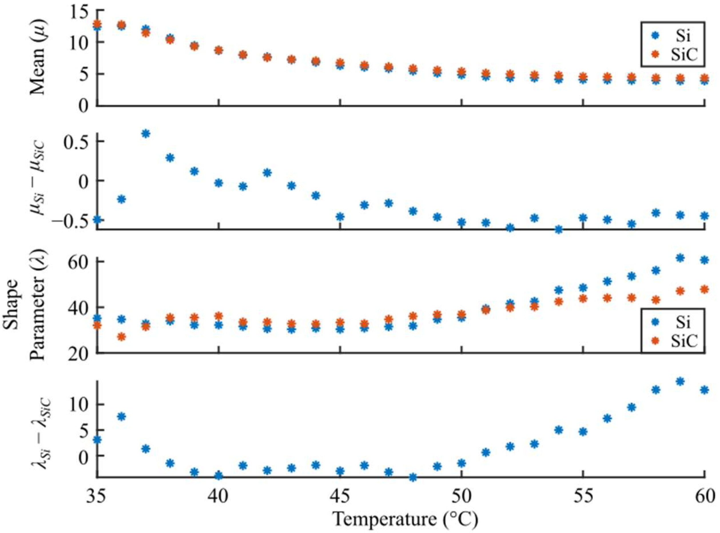
5.4. Inverse Gaussian Analysis

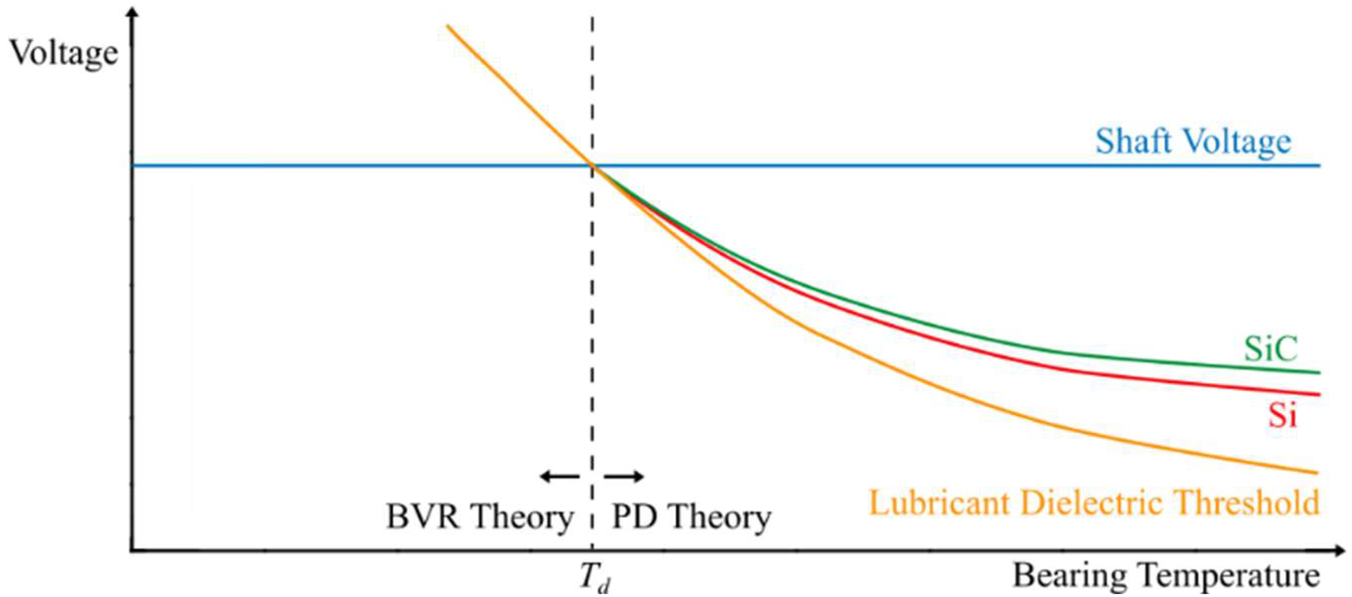
The variation in shaft breakdown voltage and peak bearing current at each operational temperature can be described with an inverse Gaussian distribution, where the sample mean µ and the shape parameter λ describe the distribution. Only the shaft voltage will be considered in this analysis, since it has been demonstrated that the shaft voltage is the causal factor for lubricant film breakdown and EDM bearing currents. The peak apparent bearing current distributions for a given operational temperature can be calculated from the modeling of Section 3 by using the shaft voltage initial breakdown conditions, for both modified and unmodified machines. The generic form of the inverse Gaussian distribution is shown in Equation (8).

$$f\left(V_{shaft},\mu ,\lambda \right)=\sqrt{\frac{\lambda }{2\pi V_{shaft}{}^3}}{e}^{\left(-\frac{\lambda {\left(V_{shaft}-\mu \right)}^2}{2{\mu }^2{V}_{shaft}}\right)}$$

(8)

The inverse Gaussian distributions describing the Si and SiC shaft breakdown voltages can be seen in Figure 18 for various temperatures, while Figure 19 visually demonstrates the inverse Gaussian shape of the raw data for 1000 ms of shaft breakdown voltages at a bearing temperature of 45 °C. From Figure 18, the distributions are dependent on bearing temperature. A comparison of the mean and scale parameter for Si and SiC inverter inverse Gaussian distribution functions at various operational temperatures is summarized in

Table 4. Summary of mean (µ) and shape (λ) parameters for shaft discharge voltage inverse Gaussian distributions over various bearing operational temperatures.

Bearing Temperature (°C)	Si		SiC
	µ	λ	µ	λ
35	12.3527	35.2079	12.8455	32.1061
36	12.4745	34.7524	12.7091	27.1138
37	12.0070	32.8321	11.4103	31.5019
38	10.6137	34.0036	10.3232	35.4892
39	9.4384	32.2878	9.3202	35.5080
40	8.6808	32.2458	8.7105	36.1585
41	7.9537	31.6164	8.0266	33.5604
42	7.6655	30.6267	7.5649	33.5297
43	7.2186	30.3921	7.2825	32.8228
44	6.8500	30.8592	7.0392	32.7083
45	6.3150	30.4267	6.7725	33.4267
46	6.0649	30.9156	6.3739	32.8333
47	5.8453	31.5336	6.1311	34.7440
48	5.4703	31.8667	5.8569	36.0973
49	5.1271	34.7397	5.5887	36.8487
50	4.8606	35.4712	5.3871	36.9513
51	4.5872	39.3704	5.1204	38.7430
52	4.4020	41.6240	4.9985	39.8471
53	4.3783	42.5335	4.8522	40.2537
54	4.1525	47.5079	4.7711	42.4918
55	4.1232	48.5210	4.5945	43.8452
56	4.0623	51.3341	4.5568	44.0631
57	3.9937	53.5966	4.5423	44.1554
58	3.9755	56.1018	4.3837	43.2468
59	3.9337	61.6098	4.3703	47.1179
60	3.9279	60.6665	4.3743	47.8430

, and shown visually in Figure 20.

Difference plots are also provided in Figure 20 to see the difference between the Si and SiC distribution parameters. A slight difference in the distribution mean can be seen at temperatures greater than 45 °C (greater than 50% of machine full load) and a significant difference in the distribution shape parameter develops above 50 °C. For temperatures below 45 °C, the trend of the differences between the distribution parameters are not as strong, although the plots of Figure 17 still suggest that shaft voltages due to SiC inverters have slightly larger magnitudes in this region. As the temperature increases, the decreasing mean shows how the distribution of shaft breakdown voltages are shifted to lower values, while the increasing shape parameter helps account for the discharge voltages being concentrated into a narrower value of voltages, becoming less right skewed with an increase in temperature. When comparing the devices, the relatively larger mean and lower shape parameters of the SiC inverter shows that the distributions cluster more narrowly at a lower shaft breakdown voltage for the Si inverter. The smaller shape parameter exhibited by the SiC inverter at temperatures greater than 50 °C demonstrates that these distributions are more skewed to higher energy values than the Si inverter distributions at the same temperature, which means that the amplitude of shaft breakdown voltages is larger in this region for the SiC inverter. Therefore, although EDM discharges due to shaft voltages and bearing currents are most intense at lightly loaded conditions, the greatest difference between EDM discharges for Si and SiC devices is seen at bearing temperatures greater than 50 °C (>75% of rated machine load). These results indicate that substantial differences in bearing lifetime may be seen when driving a machine at rated load with SiC devices, compared to Si devices.

5.5. Discussion

As previously mentioned, various researchers have demonstrated that the voltage slew rate of a voltage pulse applied across a dielectric significantly affects the breakdown voltage magnitude [32,33,34,35,36]. Wang et al. [32] developed a mathematical model to predict an expectation breakdown voltage given an inception voltage, a maximum possible breakdown voltage, an exponentially probabilistic function that describes the electron delay time of the system, and a slew rate of the applied voltage pulse. Applied to the bearing discharge phenomena, the expectation voltage is the predicted breakdown voltage, the inception voltage is the bearing lubricant dielectric breakdown voltage at dc, and the maximum possible voltage is set by the system’s voltage source, which would be the shaft voltage due to the BVR. The model effectively demonstrates how voltage pulses with higher slew rates produce larger expectation voltages at breakdown, given that all other parameters are fixed. Unfortunately, this mathematical method contains too many degrees of freedom to apply to the physics considered in this paper. Nevertheless, the concept remains a valid framework for analyzing electrical discharge behavior in motor bearings for alterations in the semiconductor device slew rate and contains the underlying principle that connects the BVR theory with the pulsed dielectric theory. As previously discussed, the BVR is a function of the machine parasitic capacitances. The changes of these parasitics that set the BVR are negligible across operational temperature, therefore the voltage that attempts to build on the shaft as produced by the CM voltage remains constant in amplitude throughout bearing temperature. However, the threshold for lubricant dielectric breakdown decreases with an increase in temperature, as has been experimentally and statistically demonstrated in this chapter. The temperature T_d at which the threshold for bearing lubricant dielectric breakdown becomes equal to the maximum shaft voltage is where the first bearing discharges appear, as seen in Figure 21.

In Figure 21, the blue line represents the shaft voltage as set by the BVR. The yellow line represents the dc threshold for bearing lubricant dielectric breakdown. Above T_d the shaft voltage set by the BVR exceeds the lubricant dielectric threshold, resulting in discharges. Therefore, BVR theory explains the shaft voltage amplitude below T_d, while pulse dielectric theory explains shaft voltage amplitude above T_d. Connecting to the work performed by Wang et al., the lubricant dielectric threshold (orange) represents the inception voltage, while the shaft voltage as set by BVR theory represents the maximum possible breakdown voltage. Since the inception voltage of the lubricant is greater than the maximum possible voltage on the shaft in the BVR region (Bearing Temperature < T_d), no discharges occur, the lubricant remains intact, and the shaft voltage is a fraction of the CM voltage as set by the BVR. Above T_d, the inception voltage drops below the maximum possible breakdown voltage, allowing discharges to occur. As the temperature increases, the difference between the maximum possible shaft voltage as set by the BVR and the inception voltage increases, and therefore the slew rate of the semiconductor switching devices begins to affect the expectation voltage for shaft breakdown. The increasing difference between the maximum possible shaft voltage and the lubricant dielectric threshold as the bearing temperature increases is the reason that the difference in expectation breakdown voltage between Si and SiC switching devices becomes more apparent with an increase in temperature. This explains why only a small difference between Si and SiC shaft breakdown voltages can be seen below 50 °C, and the difference between the devices becomes larger and much more significant above 50 °C.

6. Conclusions

This paper presented discharge modeling and a statistical analysis of shaft voltages and EDM bearing currents in a 5 hp IM driven by both Si- and SiC-based PWM inverters.

Through circuit modeling in PSpice, it was shown that the measurement methods researchers use to obtain experimental data of EDM bearing currents alters the discharge profile. The measurement wire introduces a parasitic into the discharge path that dampens the peak value of the discharge. By finding the discharge parasitic component values, a calculation can be made to deduce the EDM bearing current profile in an unmodified machine.

The EDM discharges in an electric machine are often characterized by the worst-case scenario discharge, but in fact follow a distribution, as has been shown. Considering the correlation between EDM discharge energy and the rate of bearing damage and vibration accumulation, and given that the EDM rate is linearly proportional to the PWM switching frequency [14], it becomes necessary to characterize the amplitudes of the EDM discharges over various operating conditions and know the number of discharges that have occurred to enable a bearing lifetime prediction. Therefore, the work presented here is a key step in the development of model predictive research for bearing lifetime. Additionally, the methods developed in this paper can be applied to any motor drive system that produces CM voltages from PWM inverters, including multi-level and multi-phase systems. The advantage of the techniques presented here is that precise discharge energies can be computed from the acquired motor parasitic capacitances, which will vary greatly across hp range and machine type.

The results presented showed that the worst shaft voltages and bearing currents occurred at lightly loaded conditions where the bearing lubricant film is thick, and as the film becomes thinner at higher temperatures, the magnitude of the shaft voltages and EDM bearing currents decreased. Overall, SiC devices cause higher shaft voltages and EDM bearing currents when compared to Si devices, and this phenomenon becomes significant at machine loads greater than 75% of rated load. Therefore, a significant difference in bearing lifetime may be observed between Si- and SiC-driven machines, given that a machine is typically operated above 75% of rated load to maximize its economic investment.

References

1. Ferreira, F.J.T.E.; Baoming, G.; de Almeida, A.T. Reliability and Operation of High-Efficiency Induction Motors. IEEE Trans. Ind. Appl. 2016, 52, 4628–4637. [Google Scholar] [CrossRef]
2. Bonnett, A. Root Cause Methodology for Induction Motors: A Step-by-Step Guide to Examining Failure. IEEE Ind. Appl. Mag. 2012, 18, 50–62. [Google Scholar] [CrossRef]
3. Thorsen, O.V.; Dalva, M. A survey of faults on induction motors in offshore oil industry, petrochemical industry, gas terminals, and oil refineries. IEEE Trans. Ind. Appl. 1995, 31, 1186–1196. [Google Scholar] [CrossRef]
4. Zhang, P.J.; Du, Y.; Habetler, T.G.; Lu, B. A Survey of Condition Monitoring and Protection Methods for Medium-Voltage Induction Motors. IEEE Trans. Ind. Appl. 2011, 47, 34–46. [Google Scholar] [CrossRef]
5. Nandi, S.; Toliyat, H.A.; Li, X. Condition Monitoring and Fault Diagnosis of Electrical Motors—A Review. IEEE Trans. Energy Convers. 2005, 20, 719–729. [Google Scholar] [CrossRef]
6. Muetze, A. Bearing Currents in Inverter-Fed AC-Motors; Darmstadt University of Technology, Shaker Verlag: Aachen, Germany, 2004. [Google Scholar]
7. Erdman, J.M.; Kerkman, R.J.; Schlegel, D.W.; Skibinski, G.L. Effect of PWM inverters on AC motor bearing currents and shaft voltages. IEEE Trans. Ind. Appl. 1996, 32, 250–259. [Google Scholar] [CrossRef]
8. Ogasawara, S.; Akagi, H. Modeling and damping of high-frequency leakage currents in PWM inverter-fed AC motor drive systems. IEEE Trans. Ind. Appl. 1996, 32, 1105–1114. [Google Scholar] [CrossRef] [Green Version]
9. Muetze, A.; Binder, A. Calculation of Motor Capacitances for Prediction of the Voltage Across the Bearings in Machines of Inverter-Based Drive Systems. IEEE Trans. Ind. Appl. 2007, 43, 665–672. [Google Scholar] [CrossRef]
10. Busse, D.; Erdman, J.; Kerkman, R.J.; Schlegel, D.; Skibinski, G. System electrical parameters and their effects on bearing currents. IEEE Trans. Ind. Appl. 1997, 33, 577–584. [Google Scholar] [CrossRef]
11. Chen, S.; Lipo, T.A.; Fitzgerald, D. Source of induction motor bearing currents caused by PWM inverters. IEEE Trans. Energy Convers. 1996, 11, 25–32. [Google Scholar] [CrossRef]
12. Erdman, A.; Binder, A. Calculation of Circulating Bearing Currents in Machines of Inverter-Based Drive Systems. IEEE Trans. Ind. Electron. 2007, 54, 932–938. [Google Scholar]
13. Boyanton, H.E.; Hodges, G. Bearing fluting [motors]. IEEE Ind. Appl. Mag. 2002, 8, 53–57. [Google Scholar] [CrossRef]
14. Muetze, A.; Binder, A.; Vogel, H.; Hering, J. What can bearings bear? IEEE Ind. Appl. Mag. 2006, 12, 57–64. [Google Scholar] [CrossRef]
15. Busse, D.F.; Erdman, J.M.; Kerkman, R.J.; Schlegel, D.W.; Skibinski, G.L. The effects of PWM voltage source inverters on the mechanical performance of rolling bearings. IEEE Trans. Ind. Appl. 1997, 33, 567–576. [Google Scholar] [CrossRef]
16. Muetze, A.; Binder, A. Practical Rules for Assessment of Inverter-Induced Bearing Currents in Inverter-Fed AC Motors up to 500 kW. IEEE Trans. Ind. Electron. 2007, 54, 1614–1622. [Google Scholar] [CrossRef]
17. Busse, D.; Erdman, J.; Kerkman, R.J.; Schlegel, D.; Skibinski, G. Bearing currents and their relationship to PWM drives. IEEE Trans. Power Electron. 1997, 12, 243–252. [Google Scholar] [CrossRef] [Green Version]
18. Morya, A.K.; Gardner, M.C.; Anvari, B.; Liu, L.; Yepes, A.G.; Doval-Gandoy, J.; Toliyat, H.A. Wide Bandgap Devices in AC Electric Drives: Opportunities and Challenges. IEEE Trans. Transp. Electrif. 2019, 5, 3–20. [Google Scholar] [CrossRef]
19. Xu, Y.; Yuan, X.; Ye, F.; Wang, Z.; Zhang, Y.; Diab, M.; Zhou, W. Impact of High Switching Speed and High Switching Frequency of Wide-Bandgap Motor Drives on Electric Machines. IEEE Access 2021, 9, 82866–82880. [Google Scholar] [CrossRef]
20. Xu, Y.; Liang, Y.; Yuan, X.; Wu, X.; Li, Y. Experimental Assessment of High Frequency Bearing Currents in an Induction Motor Driven by a SiC Inverter. IEEE Access 2021, 9, 40540–40549. [Google Scholar] [CrossRef]
21. Magdun, O.; Gemeinder, Y.; Binder, A. Investigation of influence of bearing load and bearing temperature on EDM bearing currents. In Proceedings of the 2010 IEEE Energy Conversion Congress and Exposition, Atlanta, GA, USA, 12–16 September 2010; pp. 2733–2738. [Google Scholar]
22. Schuster, M.; Springer, J.; Binder, A. Comparison of a 1.1 kW-induction machine and a 1.5 kW-PMSM regarding common-mode bearing currents. In Proceedings of the International Symposium on Power Electronics, Electrical Drives, Automation and Motion (SPEEDAM), Amalfi, Italy, 20–22 June 2018; pp. 1–6. [Google Scholar]
23. Schuster, M.; Binder, A. Bearing currents of a 2.4 kW-PM synchronous motor fan drive with integrated frequency inverter. In Proceedings of the 19th European Conference on Power Electronics and Applications (EPE’17 ECCE Europe), Warsaw, Poland, 11–14 September 2017; pp. 1–10. [Google Scholar]
24. Muetze, A.; Binder, A. Don’t lose your bearings. IEEE Ind. Appl. Mag. 2006, 12, 22–31. [Google Scholar] [CrossRef]
25. Schuster, M.; Masendorf, D.; Binder, A. Two PMSMs and the influence of their geometry on common-mode bearing currents. In Proceedings of the XXII International Conference on Electrical Machines (ICEM), Lausanne, Switzerland, 4–7 September 2016; pp. 2126–2132. [Google Scholar]
26. Collin, R.; Von Jouanne, A.; Yokochi, A. Novel Characterization of Si- and SiC-based PWM Inverter Bearing Currents Using Probability Density Functions. In Proceedings of the IEEE Energy Conversion Congress and Exposition, Vancouver, BC, Canada, 10–14 October 2021. [Google Scholar]
27. Zhu, N. Common-Mode Voltage Mitigation by Novel Integrated Chokes and Modulation Techniques in Power Converter Systems. Ph.D. Thesis, Ryerson University, Toronto, ON, Canada, 2013. [Google Scholar]
28. Wei, S.; Zargari, N.; Wu, B.; Rizzo, S. Comparison and mitigation of common mode voltage in power converter topologies. In Conference Record of the 2004 IEEE Industry Applications Conference, 2004. 39th IAS Annual Meeting, Seattle, WA, USA, 3–7 October 2004; IEEE: New York, NY, USA, 2004; Volume 3, pp. 1852–1857. [Google Scholar]
29. Plazenet, T.; Boileau, T.; Caironi, C.; Nahid-Mobarakeh, B. An overview of shaft voltages and bearing currents in rotating machines. In Proceedings of the 2016 IEEE Industry Applications Society Annual Meeting, Portland, OR, USA, 2–6 October 2016; pp. 1–8. [Google Scholar]
30. Jaritz, M.; Jaeger, C.; Bucher, M.; Smajic, J.; Vukovic, D.; Blume, S. An Improved Model for Circulating Bearing Currents in Inverter-Fed AC Machines. In Proceedings of the 2019 IEEE International Conference on Industrial Technology (ICIT), Melbourne, Australia, 13–15 February 2019; pp. 225–230. [Google Scholar]
31. Singleton, R.K.; Strangas, E.G.; Aviyente, S. The Use of Bearing Currents and Vibrations in Lifetime Estimation of Bearings. IEEE Trans. Ind. Inform. 2017, 13, 1301–1309. [Google Scholar] [CrossRef]
32. Wang, P.; Cavallini, A.; Montanari, G.C.; Wu, G. Effect of rise time on PD pulse features under repetitive square wave voltages. IEEE Trans. Dielectr. Electr. Insul. 2013, 20, 245–254. [Google Scholar] [CrossRef]
33. Wilson, M.P.; Timoshkin, I.V.; Given, M.J.; Macgregor, S.J.; Sinclair, M.A.; Thomas, K.J.; Lehr, J.M. Effect of applied field and rate of voltage rise on surface breakdown of oil-immersed polymers. IEEE Trans. Dielectr. Electr. Insul. 2011, 18, 1003–1010. [Google Scholar] [CrossRef] [Green Version]
34. Jadidian, J.; Zahn, M.; Lavesson, N.; Widlund, O.; Borg, K. Effects of Impulse Voltage Polarity, Peak Amplitude, and Rise Time on Streamers Initiated from a Needle Electrode in Transformer Oil. IEEE Trans. Plasma Sci. 2012, 40, 909–918. [Google Scholar] [CrossRef] [Green Version]
35. Wu, S.; Xu, H.; Lu, X.; Pan, Y. Effect of Pulse Rising Time of Pulse dc Voltage on Atmospheric Pressure Non-Equilibrium Plasma. Plasma Process. Polym. 2013, 10, 136–140. [Google Scholar] [CrossRef]
36. Babaeva, N.Y.; Naidis, G.V. Modeling of Streamer Dynamics in Atmospheric-Pressure Air: Influence of Rise Time of Applied Voltage Pulse on Streamer Parameters. IEEE Trans. Plasma Sci. 2016, 44, 899–902. [Google Scholar] [CrossRef]
37. Bubert, A.; Zhang, J.; De Doncker, R.W. Modeling and measurement of capacitive and inductive bearing current in electrical machines. In Proceedings of the 2017 Brazilian Power Electronics Conference, Juiz de Fora, Brazil, 19–22 November 2017; pp. 1–6. [Google Scholar]
38. Collin, R.; Stephens, M.; Von Jouanne, A. Development of SiC-Based Motor Drive Using Typhoon HIL 402 as System-Level Controller. In Proceedings of the IEEE Energy Conversion Congress and Exposition, Detroit, MI, USA, 11–15 October 2020. [Google Scholar]
39. Wittek, E.; Kriese, M.; Tischmacher, H.; Gattermann, S.; Ponick, B.; Poll, G. Capacitances and lubricant film thicknesses of motor bearings under different operating conditions. In Proceedings of the XIX International Conference on Electrical Machines—ICEM, Rome, Italy, 6–8 September 2010; pp. 1–6. [Google Scholar]
40. BenSaida, A. Shapiro-Wilk and Shapiro-Francia Normality Tests, Version 1.1.0.0; MATLAB Central File Exchange: Natick, MA, USA, 2021. [Google Scholar]
Figure 1. The high frequency components of the inverter CM voltage excite a CM current through the parasitic capacitive paths in a machine.
Energies 15 03043 g001
Figure 2. A typical three-phase ac-dc-ac motor drive power electronic converter for lower power applications (<25 hp). The ac grid input voltages are converted to dc via a three-phase diode bridge rectifier. A two-level six-switch inverter then synthesizes the dc bus into the PWM phase voltages necessary to drive the machine, which is depicted with a low frequency RL model. The inverter CM voltage is a result of the PWM phase voltages.
Energies 15 03043 g002
Figure 3. (a) EDM currents produce pits and pillars on the race surface as seen in this scanning electron microscope (SEM) image at 1000× magnification (b) that appears as frosting on a macroscopic level.
Energies 15 03043 g003
Figure 4. Circuit model of EDM bearing current paths in an electric machine with the effects of motor modification for bearing current measurement included. For an unmodified machine, the components Ci and Lw are not a part of the discharge path.
Energies 15 03043 g004
Figure 5. A 17 V, 700 mA discharge measured experimentally at a discharge frequency of 10.33 MHz.
Energies 15 03043 g005
Figure 6. Experimental testbed constructed for the acquisition of shaft voltages and EDM bearing currents for Si- and SiC-based PWM inverters.
Energies 15 03043 g006
Figure 7. Modified induction motor bearing discharge equivalent circuit model.
Energies 15 03043 g007
Figure 8. Equivalent parasitic circuit model for (a) zero speed and (b) rated speed conditions. The bearing is a short circuit at zero speed due to direct contact between the balls and races, while the bearing behaves as a capacitance at rated speed due to the balls riding on a film of lubricant.
Energies 15 03043 g008
Figure 9. Experimental and PSpice simulation waveforms for a 20 V, 1150 mA discharge.
Energies 15 03043 g009
Figure 10. A 23 V shaft voltage discharge that takes ~17 ns to discharge on the unmodified IM.
Energies 15 03043 g010
Figure 11. Unmodified induction motor bearing discharge equivalent circuit model.
Energies 15 03043 g011
Figure 12. Simulated EDM bearing current for a 23 V shaft voltage discharge that dissipates in ~17 ns.
Energies 15 03043 g012
Figure 13. Shaft discharge voltage and peak apparent bearing current data for various bearing operational temperatures: 3D plots for (a) Si and (b) SiC inverters. 2D plots comparing shaft discharge voltages against operational temperature for (c) Si and (d) SiC inverters, and 2D plots displaying the peak apparent bearing currents for a given shaft breakdown voltage for (e) Si and (f) SiC inverters.
Energies 15 03043 g013aEnergies 15 03043 g013b
Figure 14. The resulting peak apparent bearing current follows a normal distribution for any particular shaft breakdown voltage, in this case for the SiC inverter 9.7 V discharges at 42 °C: (a) histogram of experimental data with fitted theoretical normal distribution, (b) cumulative density plot comparing data (blue) with theoretical normal distributions (orange), and (c) probability plot demonstrating the normally distributed data.
Energies 15 03043 g014
Figure 15. Probability plot of the raw SiC 9.7 V, 42 °C peak apparent bearing current data.
Energies 15 03043 g015
Figure 16. The normally distributed peak apparent bearing current is due to a normally distributed bearing discharge resistance.
Energies 15 03043 g016
Figure 17. Comparison of maximum shaft discharge voltages at various bearing operational temperatures for Si and SiC inverters, with line-driven operation included.
Energies 15 03043 g017
Figure 18. Si and SiC inverter shaft breakdown voltage inverse Gaussian distributions for various bearing operational temperatures.
Energies 15 03043 g018
Figure 19. Histogram with inverse Gaussian distribution and probability plot for SiC inverter shaft breakdown voltage data at a bearing temperature of 45 °C. In 1000 ms at fs = 10 kHz, 8006 discharge events were recorded.
Energies 15 03043 g019
Figure 20. Mean and shape parameters of the shaft breakdown voltage inverse Gaussian distributions plotted against temperature.
Energies 15 03043 g020
Figure 21. Comparison of the lubricant dielectric threshold at dc (yellow), and shaft discharge voltages produced by Si (red) and SiC (green) inverters. The shaft voltage amplitude as set by the BVR is shown in blue. The temperature at which discharges are first observed is denoted Td.
Energies 15 03043 g021