
Two-Dimensional Gravity Inversion of Basement Relief for Geothermal Energy Potentials at the Harrat Rahat Volcanic Field, Saudi Arabia, Using Particle Swarm Optimization


Abstract
:1. Introduction
Geological Setting
2. Materials and Methods
2.1. Data Acquisition and Processing
2.2. Methodology
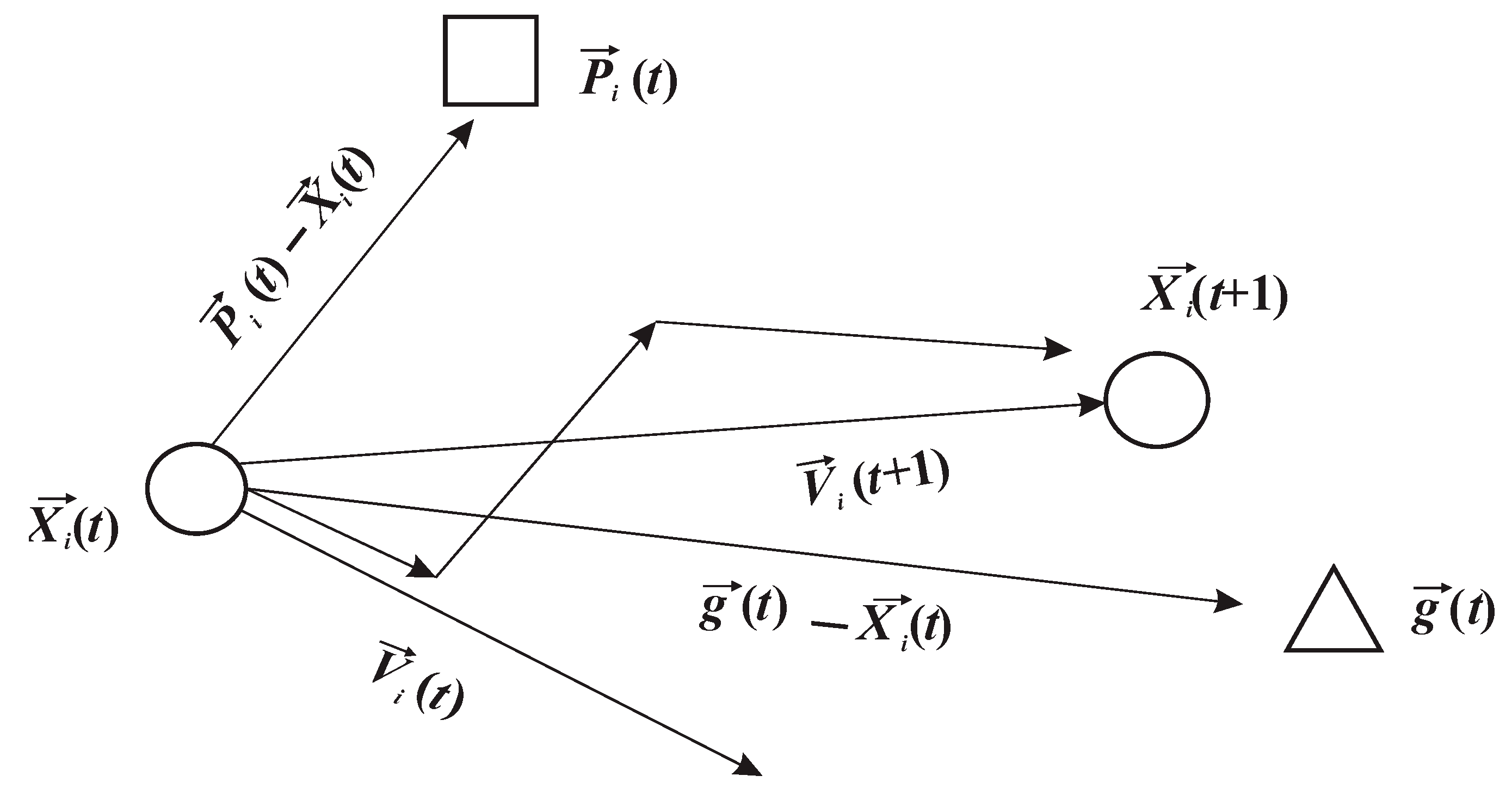
2.3. Particle Swarm Optimization (PSO)
2.4. The Euler Deconvolution of the Aeromagnetic Data
3. Results
4. Discussion
5. Conclusions
Author Contributions
Funding
Institutional Review Board Statement
Informed Consent Statement
Data Availability Statement
Acknowledgments
Conflicts of Interest
References
- Al-Amri, A.M.; Mellors, R.; Harris, D.; El-Sayed, K.A. Geothermal and Volcanic Evaluation of Harrat Rahat, Northwestern Arabian Peninsula; Profect No.: 11-SPA 2208-02; National Plan for Science, Tech. & Innovation; King Saud University: Riyadh, Saudi Arabia, 2016. [Google Scholar]
- Al-Shijbi, Y.; El-Hussain, I.; Deif, A.; Al-Kalbani, A.; Mohamed, A.M.E. Probabilistic Seismic Hazard Assessment for the Arabian Peninsula. Pure Appl. Geophys. 2019, 176, 1503–1530. [Google Scholar] [CrossRef]
- Zahran, H.M.; Sokolov, V.; Roobol, M.J.; Stewart, I.C.F.; Youssef, S.; Elhadidy, M. On the development of a seismic source zonation model for seismic hazard assessment in western Saudi Arabia. J. Seism. 2016, 20, 747–769. [Google Scholar] [CrossRef]
- Wilson, J.W.P.; Roberts, G.G.; Hoggard, M.J.; White, N.J. Cenozoic epeirogeny of the Arabian Peninsula from drainage modeling. Geochem. Geophys. Geosystems 2014, 15, 3723–3761. [Google Scholar] [CrossRef]
- Niazi, M. Crustal Thickness in the Central Saudi Arabian Peninsula. Geophys. J. Int. 1968, 15, 545–547. [Google Scholar] [CrossRef] [Green Version]
- El-Hussain, I.; Al-Shijbi, Y.; Deif, A.; Mohamed, A.M.E.; Ezzelarab, M. Developing a seismic source model for the Arabian Plate. Arab. J. Geosci. 2018, 11, 435. [Google Scholar] [CrossRef]
- Deif, A.; Al-Shijbi, Y.; El-Hussain, I.; Ezzelarab, M.; Mohamed, A.M. Compiling an earthquake catalogue for the Arabian Plate, Western Asia. J. Southeast Asian Earth Sci. 2017, 147, 345–357. [Google Scholar] [CrossRef]
- Stern, R.J.; Johnson, P. Continental lithosphere of the Arabian Plate: A geologic, petrologic, and geophysical synthesis. Earth-Sci. Rev. 2010, 101, 29–67. [Google Scholar] [CrossRef]
- ArRajehi, A.; McClusky, S.; Reilinger, R.; Daoud, M.; Alchalbi, A.; Ergintav, S.; Gomez, F.; Sholan, J.; Bou-Rabee, F.; Ogubazghi, G.; et al. Geodetic constraints on present-day motion of the Arabian Plate: Implications for Red Sea and Gulf of Aden rifting. Tectonics 2010, 29, TC3011. [Google Scholar] [CrossRef] [Green Version]
- Berthier, F.; Demange, J.; Iundt, F.; Verzier, P. Geothermal Resources of the Kingdom of Saudi Arabia; Saudi Arabian Deputy Ministry for Mineral Resources Open-File Report BRGM-OF-01-24; Ministry of Petroleum and Mineral Resources: Jiddah, Saudi Arabia, 1981; p. 116. [Google Scholar]
- Rehman, S.; Shash, A. Geothermal Resources of Saudi Arabia—Country Update Report. In Proceedings of the World Geothermal Congress 2005, Antalya, Turkey, 24–29 April 2005. [Google Scholar]
- Rehman, S. Saudi Arabian Geothermal Energy Resources—An Update. In Proceedings of the World Geothermal Congress 2010, Bali, Indonesia, 25–29 April 2010. [Google Scholar]
- Demirbas, A.; Alidrisi, H.; Ahmad, W.; Sheikh, M.H. Potential of geothermal energy in the Kingdom of Saudi Arabia. Energy Sources Part A Recover. Util. Environ. Eff. 2016, 38, 2238–2243. [Google Scholar] [CrossRef]
- Al-Dayel, M. Geothermal resources in Saudi Arabia. Geothermics 1988, 17, 465–476. [Google Scholar] [CrossRef]
- Roobol, M.J.; Bankher, K.; Bamufleh, S. Geothermal Anomalies along the MMN Volcanic Line Including the Cities of Al Madinah Al Munnawwarah and Makkah Al Mukkarramah; Saudi Geological Survey: Jeddah, Saudi Arabia, 2007. [Google Scholar]
- Lashin, A.; Al Arifi, N. Geothermal energy potential of southwestern of Saudi Arabia “exploration and possible power generation”: A case study at AlKhouba area–Jizan. Renew. Sustain. Energy Rev. 2014, 30, 771–789. [Google Scholar] [CrossRef]
- Lashin, A.; Al Arifi, N.; Chandrasekharam, D.; Al Bassam, A.; Rehman, S.; Pipan, M. Geothermal Energy Resources of Saudi Arabia: Country Update. In Proceedings of the World Geothermal Congress 2015, Melbourne, Australia, 19–25 April 2015. [Google Scholar]
- Hussein, M.T.; Lashin, A.; Al Bassam, A.; Al-Arifi, N.; Al Zahrani, I. Geothermal power potential at the western coastal part of Saudi Arabia. Renew. Sustain. Energy Rev. 2013, 26, 668–684. [Google Scholar] [CrossRef] [Green Version]
- Lashin, A.; Al Arifi, N. The geothermal potential of Jizan area, Southwestern parts of Saudi Arabia. Int. J. Phys. Sci. 2012, 4, 664–675. [Google Scholar]
- Berthier, F.; Demange, J.; Iundt, F. Geothermal Resources of Harrat Khaybar and Harrat Rahat Progress Report 1400-1401 the Kingdom of Saudi Arabia; Saudi Arabian Deputy Ministry for Mineral Resources Open-File Report BRGM-OF-02-44; Ministry of Petroleum and Mineral Resources: Jiddah, Saudi Arabia, 1982; p. 116. [Google Scholar]
- Zahran, H.; Stewart, I.C.F.; Johnson, P.R.; Basahel, M.H. Aeromagnetic-anomaly maps of central and western Saudi Arabia. In Saudi Geological Survey Open-File Report SGS-OF-2002-8; 4 Plates; 2003; p. 6. [Google Scholar]
- Al-Douri, Y.; Waheeb, S.; Johan, M.R. Exploiting of geothermal energy reserve and potential in Saudi Arabia: A case study at Ain Al Harrah. Energy Rep. 2019, 5, 632–638. [Google Scholar] [CrossRef]
- Civilini, F.; Mooney, W.D.; Savage, M.K.; Townend, J.; Zahran, H. Crustal imaging of northern Harrat Rahat, Saudi Arabia, from ambient noise tomography. Geophys. J. Int. 2019, 219, 1532–1549. [Google Scholar] [CrossRef]
- Abdelwahed, M.F.; El-Masry, N.; Moufti, M.R.; Kenedi, C.L.; Zhao, D.; Zahran, H.; Shawali, J. Imaging of magma intrusions beneath Harrat Al-Madinah in Saudi Arabia. J. Southeast Asian Earth Sci. 2016, 120, 17–28. [Google Scholar] [CrossRef]
- Aboud, E.; Wameyo, P.; Alqahtani, F.; Moufti, M. Imaging subsurface northern Rahat Volcanic Field, Madinah city, Saudi Arabia, using Magnetotelluric study. J. Appl. Geophys. 2018, 159, 564–572. [Google Scholar] [CrossRef]
- Murcia, H.; Németh, K.; Moufti, M.R.; Lindsay, J.M.; El-Masry, N.; Cronin, S.; Qaddah, A.; Smith, I.E.M. Late Holocene lava flow morphotypes of northern Harrat Rahat, Kingdom of Saudi Arabia: Implications for the description of continental lava fields. J. Southeast Asian Earth Sci. 2013, 84, 131–145. [Google Scholar] [CrossRef]
- Langenheim, V.E.; Ritzinger, B.T.; Zahran, H.; Shareef, A.; Al-Dahri, M. Crustal structure of the northern Harrat Rahat volcanic field (Saudi Arabia) from gravity and aeromagnetic data. Tectonophysics 2018, 750, 9–21. [Google Scholar] [CrossRef]
- Aboud, E.; El-Masry, N.; Qaddah, A.; Alqahtani, F.; Moufti, M.R.H. Magnetic and gravity data analysis of Rahat volcanic field, El-Madinah city, Saudi Arabia. NRIAG J. Astron. Geophys. 2015, 4, 154–162. [Google Scholar] [CrossRef] [Green Version]
- Blank, H.R.; Sadek, H.S. Spectral Analysis of the 1976 Aeromagnetic Survey of Harrat Rahat, Kingdom of Saudi Arabia; Saudi Arabian Deputy Ministry for Mineral Resources Open-File Report USGS-OF-03-67; Ministry of Petroleum and Mineral Resources: Jiddah, Saudi Arabia, 1983; p. 29. [Google Scholar]
- Roy, A.; Dubey, C.P.; Prasad, M. Gravity inversion of basement relief using Particle Swarm Optimization by automated parameter selection of Fourier coefficients. Comput. Geosci. 2021, 156, 104875. [Google Scholar] [CrossRef]
- Singh, K.K.; Singh, U.K. Application of particle swarm optimization for gravity inversion of 2.5-D sedimentary basins using variable density contrast. Geosci. Instrum. Methods Data Syst. 2017, 6, 193–198. [Google Scholar] [CrossRef] [Green Version]
- Rama Rao, B.S.; Murthy, I.V.R. Gravity and Magnetic Methods of Prospecting; Arnold-Heinemann: New Delhi, India, 1978. [Google Scholar]
- Won, I.J.; Bevis, M. Computing the gravitational and magnetic anomalies due to a polygon: Algorithms and Fortran subroutines. Geophysics 1987, 52, 232–238. [Google Scholar] [CrossRef]
- Rao, C.V.; Pramanik, A.G.; Kumar, G.V.R.K.; Raju, M.L. Gravity interpretation of sedimentary basins with hyperbolic density contrast. Geophys. Prospect. 1994, 42, 825–839. [Google Scholar] [CrossRef]
- Murthy, I.V.R.; Rao, S.J. A FORTRAN 77 program for inverting gravity anomalies of two-dimensional basement structures. Comput. Geosci. 1989, 15, 1149–1156. [Google Scholar] [CrossRef]
- Litinsky, V.A. Concept of effective density: Key to gravity depth determinations for sedimentary basins. Geophysics 1989, 54, 1474–1482. [Google Scholar] [CrossRef]
- Barbosa, V.C.F.; Silva, J.B.C.; Medeiros, W.E. Stable inversion of gravity anomalies of sedimentary basins with non smooth basement reliefs and arbitrary density contrast variations. Geophysics 1999, 64, 754–764. [Google Scholar] [CrossRef]
- Annecchione, M.A.; Chouteau, M.; Keating, P. Gravity interpretation of bedrock topography: The case of the Oak Ridges Moraine, southern Ontario, Canada. J. Appl. Geophys. 2001, 47, 63–81. [Google Scholar] [CrossRef]
- Ekinci, Y.L.; Balkaya, C.; Göktürkler, G.; Özyalın, S. Gravity data inversion for the basement relief delineation through global optimization: A case study from the Aegean Graben System, western Anatolia, Turkey. Geophys. J. Int. 2020, 224, 923–944. [Google Scholar] [CrossRef]
- Silva, J.B.C.; Santos, D.F.; Gomes, K.P. Fast gravity inversion of basement relief. Geophysics 2014, 79, G79–G91. [Google Scholar] [CrossRef]
- Chakravarthi, V.; Shankar, G.B.K.; Muralidharan, D.; Harinarayana, T.; Sundararajan, N. An integrated geophysical approach for imaging subbasalt sedimentary basins: Case study of Jam River Basin, India. Geophysics 2007, 72, B141–B147. [Google Scholar] [CrossRef]
- Qin, P.; Huang, D.; Yuan, Y.; Geng, M.; Liu, J. Integrated gravity and gravity gradient 3D inversion using the non-linear conjugate gradient. J. Appl. Geophys. 2016, 126, 52–73. [Google Scholar] [CrossRef]
- Feng, X.; Wang, W.; Yuan, B. 3D gravity inversion of basement relief for a rift basin based on combined multinorm and normalized vertical derivative of the total horizontal derivative techniques. Geophysics 2018, 83, G107–G118. [Google Scholar] [CrossRef]
- Montesinos, F.G.; Arnoso, J.; Vieira, R. Using a genetic algorithm for 3-D inversion of gravity data in Fuerteventura (Canary Islands). Geol. Rundsch. 2005, 94, 301–316. [Google Scholar] [CrossRef]
- Biswas, A. Interpretation of residual gravity anomaly caused by simple shaped bodies using very fast simulated annealing global optimization. Geosci. Front. 2015, 6, 875–893. [Google Scholar] [CrossRef] [Green Version]
- Toushmalani, R. Gravity inversion of a fault by Particle swarm optimization (PSO). SpringerPlus 2013, 2, 1–7. [Google Scholar] [CrossRef] [Green Version]
- Roy, A.; Kumar, T.S. Gravity inversion of 2D fault having variable density contrast using particle swarm optimization. Geophys. Prospect. 2021, 69, 1358–1374. [Google Scholar] [CrossRef]
- Pallero, J.; Fernández-Martínez, J.; Bonvalot, S.; Fudym, O. Gravity inversion and uncertainty assessment of basement relief via Particle Swarm Optimization. J. Appl. Geophys. 2015, 116, 180–191. [Google Scholar] [CrossRef]
- Pallero, J.L.G.; Fernández-Martínez, J.L.; Fernández-Martínez, Z.; Bonvalot, S.; Gabalda, G.; Nalpas, T. GRAVPSO2D: A Matlab package for 2D gravity inversion in sedimentary basins using the Particle Swarm Optimization algorithm. Comput. Geosci. 2021, 146, 104653. [Google Scholar] [CrossRef]
- Pallero, J.; Fernandez-Martinez, J.L.; Bonvalot, S.; Fudym, O. 3D gravity inversion and uncertainty assessment of basement relief via Particle Swarm Optimization. J. Appl. Geophys. 2017, 139, 338–350. [Google Scholar] [CrossRef]
- Camp, V.E.; Roobol, M.J. The Arabian continental alkali basalt province: Part I. Evolution of Harrat Rahat, Kingdom of Saudi Arabia. GSA Bull. 1989, 101, 71–95. [Google Scholar] [CrossRef]
- Downs, D.T.; Stelten, M.E.; Champion, D.E.; Dietterich, H.R.; Nawab, Z.; Zahran, H.; Hassan, K.; Shawali, J. Volcanic history of the northernmost part of the Harrat Rahat volcanic field, Saudi Arabia. Geosphere 2018, 14, 1253–1282. [Google Scholar] [CrossRef] [Green Version]
- Camp, V.E.; Hooper, P.R.; Roobol, M.J.; White, D.L. The Madinah eruption, Saudi Arabia: Magma mixing and simultaneous extrusion of three basaltic chemical types. Bull. Volcanol. 1987, 49, 489–508. [Google Scholar] [CrossRef]
- Camp, V.E.; Hooper, P.R.; Roobol, M.J.; White, D.L. The Madinah Historical Eruption: Magma Mixing and Simultaneous Extrusion of Three Basaltic Chemical Types; Saudi Arabian Directorate General of Mineral Resources, Open File Report DGMR-OF-06-32; Ministry of Petroleum and Mineral Resources: Jiddah, Saudi Arabia, 1989; p. 52. [Google Scholar]
- Camp, V.E.; Roobol, M.J. Geologic Map of the Cenozoic Lava Field of Harrat Rahat, Kingdom of Saudi Arabia; Saudi Arabian Directorate General of Mineral Resources, Geoscience Map GM-123, scale 1:250,000; Ministry of Petroleum and Mineral Resources: Jiddah, Saudi Arabia, 1991. [Google Scholar]
- Moufti, M.R.; El-Difrawy, M.A.M.; Soliman, M.A.W.; El-Moghazi, A.K.M.; Matsah, M.I. Assessing Volcanic Hazards of a Quaternary Lava Field in the Kingdom of Saudi Arabia; Final Report ARP-26-79; King Abdulaziz City for Science and Technology (KACST): Riyadh, Saudi Arabia, 2010. [Google Scholar]
- Moufti, M.R.; Moghazi, A.M.; Ali, K.A. Geochemistry and Sr–Nd–Pb isotopic composition of the Harrat Al-Madinah Volcanic Field, Saudi Arabia. Gondwana Res. 2012, 21, 670–689. [Google Scholar] [CrossRef]
- Shapiro, N.M.; Campillo, M. Emergence of broadband Rayleigh waves from correlations of the ambient seismic noise. Geophys. Res. Lett. 2004, 31, L07614. [Google Scholar] [CrossRef] [Green Version]
- Bensen, G.D.; Ritzwoller, M.H.; Barmin, M.P.; Levshin, A.L.; Lin, F.-C.; Moschetti, M.P.; Shapiro, N.; Yang, Y. Processing seismic ambient noise data to obtain reliable broad-band surface wave dispersion measurements. Geophys. J. Int. 2007, 169, 1239–1260. [Google Scholar] [CrossRef] [Green Version]
- Brenguier, F.; Shapiro, N.; Campillo, M.; Ferrazzini, V.; Duputel, Z.; Coutant, O.; Nercessian, A. Towards forecasting volcanic eruptions using seismic noise. Nat. Geosci. 2008, 1, 126–130. [Google Scholar] [CrossRef] [Green Version]
- Stankiewicz, J.; Ryberg, T.; Haberland, C.; Natawidjaja, D. Lake Toba volcano magma chamber imaged by ambient seismic noise tomography. Geophys. Res. Lett. 2010, 37, L17306. [Google Scholar] [CrossRef] [Green Version]
- Nagy, D. The gravitational attraction of a right rectangular prism. Geophysics 1966, 31, 362–371. [Google Scholar] [CrossRef]
- Kane, M.F. A comprehensive system of terrain corrections using a digital computer. Geophysics 1962, 27, 455–462. [Google Scholar] [CrossRef]
- Dobrin, M.B.; Savit, C.H. Introduction to Geophysical Prospecting, 4th ed.; McGraw-Hill Book Co.: New York, NY, USA, 1988; 867p. [Google Scholar]
- Gupta, V.K.; Ramani, N. Some aspects of regional-residual separation of gravity anomalies in a Precambrian terrain. Geophysics 1980, 45, 1412–1426. [Google Scholar] [CrossRef]
- Mickus, K.; Aiken, C.L.V.; Kennedy, W.D. Regional-residual gravity anomaly separation using the minimum-curvature technique. Geophysics 1991, 56, 279–283. [Google Scholar] [CrossRef]
- Guglielmetti, L.; Moscariello, A. On the use of gravity data in delineating geologic features of interest for geothermal exploration in the Geneva Basin (Switzerland): Prospects and limitations. Swiss J. Geosci. 2021, 114, 1–20. [Google Scholar] [CrossRef]
- Elhussein, M. New Inversion Approach for Interpreting Gravity Data Caused by Dipping Faults. Earth Space Sci. 2021, 8, e2020EA001075. [Google Scholar] [CrossRef]
- Ekinci, Y.L.; Balkaya, Ç.; Göktürkler, G.; Turan, S. Model parameter estimations from residual gravity anomalies due to simple-shaped sources using Differential Evolution Algorithm. J. Appl. Geophys. 2016, 129, 133–147. [Google Scholar] [CrossRef]
- Biswas, A.; Sharma, S.P. Interpretation of self-potential anomaly over idealized bodies and analysis of ambiguity using very fast simulated annealing global optimization technique. Near Surf. Geophys. 2015, 13, 179–195. [Google Scholar] [CrossRef]
- Heppner, H.; Grenander, U. Stochastic non-linear model for coordinated bird flocks. In The Ubiquity of Chaos; Krasner, S., Ed.; AAAS: Washington, DC, USA, 1990; pp. 233–238. [Google Scholar]
- Reynolds, C.W. Flocks, herds and schools: A distributed behavioral model. ACM SiggraphComput. Graph. 1987, 21, 25–34. [Google Scholar] [CrossRef] [Green Version]
- Kennedy, J.; Eberhart, R. Particle Swarm Optimization. In Proceedings of the ICNN’95—International Conference on Neural Networks, Perth, Australia, 27 November–1 December 1995; Volume 4, pp. 1942–1948. [Google Scholar] [CrossRef]
- Gao, Y.-L.; An, X.-H.; Liu, J.-M. A particle swarm optimization algorithm with logarithm decreasing inertia weight and chaos mutation. In Proceedings of the 2008 International Conference on Computational Intelligence and Security, Suzhou, China, 13–17 December2008; Volume 1, pp. 61–65. [Google Scholar]
- Chai, Y.; Hinze, W.J. Gravity inversion of an interface above which the density contrast varies exponentially with depth. Geophysics 1988, 53, 837–845. [Google Scholar] [CrossRef]
- Cordell, L. Gravity analysis using an exponential density-depth function—San Jacinto Graben, California. Geophysics 1973, 38, 684–690. [Google Scholar] [CrossRef]
- Kaso, A. Computation of the normalized cross-correlation by fast Fourier transform. PLoS ONE 2018, 13, e0203434. [Google Scholar] [CrossRef]
- Perez, R.; Behdinan, K. Particle swarm approach for structural design optimization. Comput. Struct. 2007, 85, 1579–1588. [Google Scholar] [CrossRef]
- Nickabadi, A.; Ebadzadeh, M.M.; Safabakhsh, R. A novel particle swarm optimization algorithm with adaptive inertia weight. Appl. Soft Comput. 2011, 11, 3658–3670. [Google Scholar] [CrossRef]
- Xin, J.; Chen, G.; Hai, Y. A particle swarm optimizer with multi-stage linearly-decreasing inertia weight. In Proceedings of the 2009 International Joint Conference on Computational Sciences and Optimization, Sanya, China, 24–26 April 2009; Volume 1, pp. 505–508. [Google Scholar]
- Malik, R.F.; Rahman, T.A.; Hashim, S.Z.M.; Ngah, R. New particle swarm optimizer with sigmoid increasing inertia weight. Int. J. Comput. Sci. Secur. 2007, 1, 35–44. [Google Scholar]
- Thompson, D.T. Euldph: A new technique, for making computer-assisted, depth- estimates, from magnetic data. Geophysics 1982, 47, 31–37. [Google Scholar] [CrossRef]
- Whitehead, N.; Musselman, C. Montaj Gravity/Magnetic Interpretation: Processing, Analysis, and Visualization System, for 3-D Inversion of Potential Field Data, for Oasis Montaj v6.1; Geosoft Inc.: Toronto, ON, Canada, 2005. [Google Scholar]
- Reid, A.B.; Allsop, J.M.; Grauser, H.; Millet, A.J.; Somerton, I.N. Magnetic interpretation in 3D using Euler Deconvolution. Geophysics 1990, 55, 80–91. [Google Scholar] [CrossRef] [Green Version]
- Abraham, E.M.; Alile, O.M. Modelling Subsurface Geologic Structures at Ikogosi Geothermal Field, Southwestern Nigeria, using Gravity, Magnetics, and Seismic Interferometry Techniques. J. Geophys. Eng. 2019, 16, 729–741. Available online: https://academic.oup.com/jge/advance-article-bstract/doi/10.1093/jge/gxz034/5531815 (accessed on 3 September 2019). [CrossRef]
- Rasmussen, R.; Pedersen, L.B. End corrections in potential field modeling. Geophys. Prospect. 1979, 27, 749–760. [Google Scholar] [CrossRef]
- Blaikie, T.N.; Ailleres, L.; Betts, P.G.; Cas, R.A.F. Interpreting subsurface volcanic structures using geologically constrained 3-D gravity inversions: Examples of maar-diatremes, Newer Volcanics Province, southeastern Australia. J. Geophys. Res. Solid Earth 2014, 119, 3857–3878. [Google Scholar] [CrossRef]
- Silva, J.B.C.; Teixeira, W.A.; Barbosa, V.C.F. Gravity data as a tool for landfill study. Environ. Geol. 2009, 57, 749. [Google Scholar] [CrossRef]
- Chen, Z.; Meng, X.; Zhang, S. 3D gravity interface inversion constrained by a few points and its GPU acceleration. Comput. Geosci. 2015, 84, 20–28. [Google Scholar] [CrossRef]
- Pellaton, C. Geologic Map of the Al Madinah Quadrangle, Sheet 24D; Kingdom of Saudi Arabia (with Text): Saudi Arabian Directorate General of Mineral Resources Geologic Map GM-52C, Scale 1:250,000; Ministry of Petroleum and Mineral Resources: Jiddah, Saudi Arabia, 1981; 19p. [Google Scholar]
- Camp, V.E. Geologic Map of the Umm Al Birak Quadrangle, Sheet 23D; Kingdom of Saudi Arabia (with Text): Saudi Arabian Directorate General of Mineral Resources Geologic Map Map GM-87C, Scale 1:250,000; Ministry of Petroleum and Mineral Resources: Jiddah, Saudi Arabia, 1986; 40p. [Google Scholar]


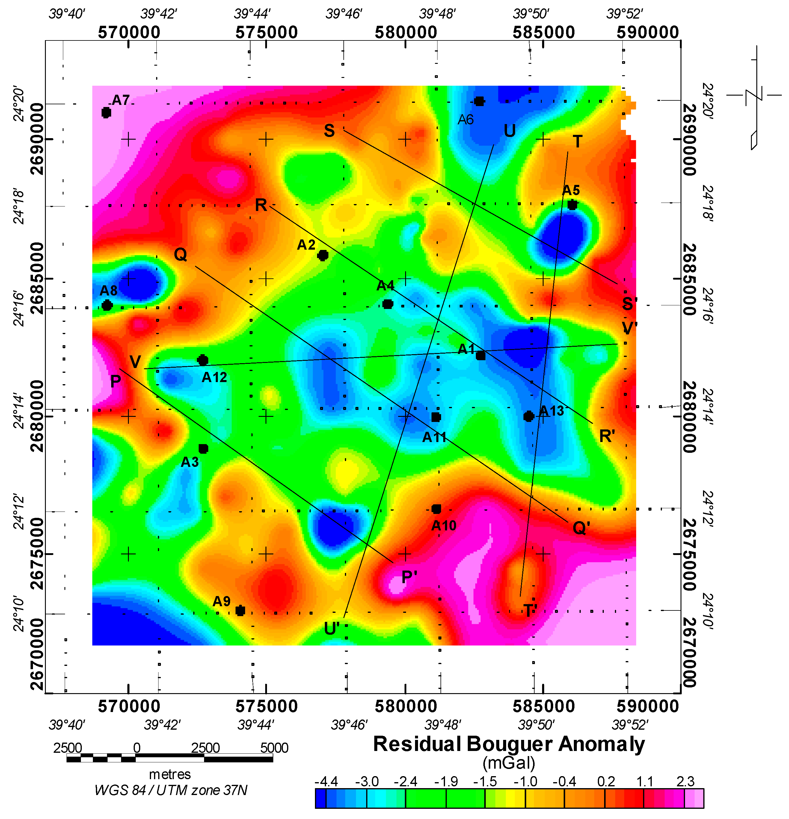
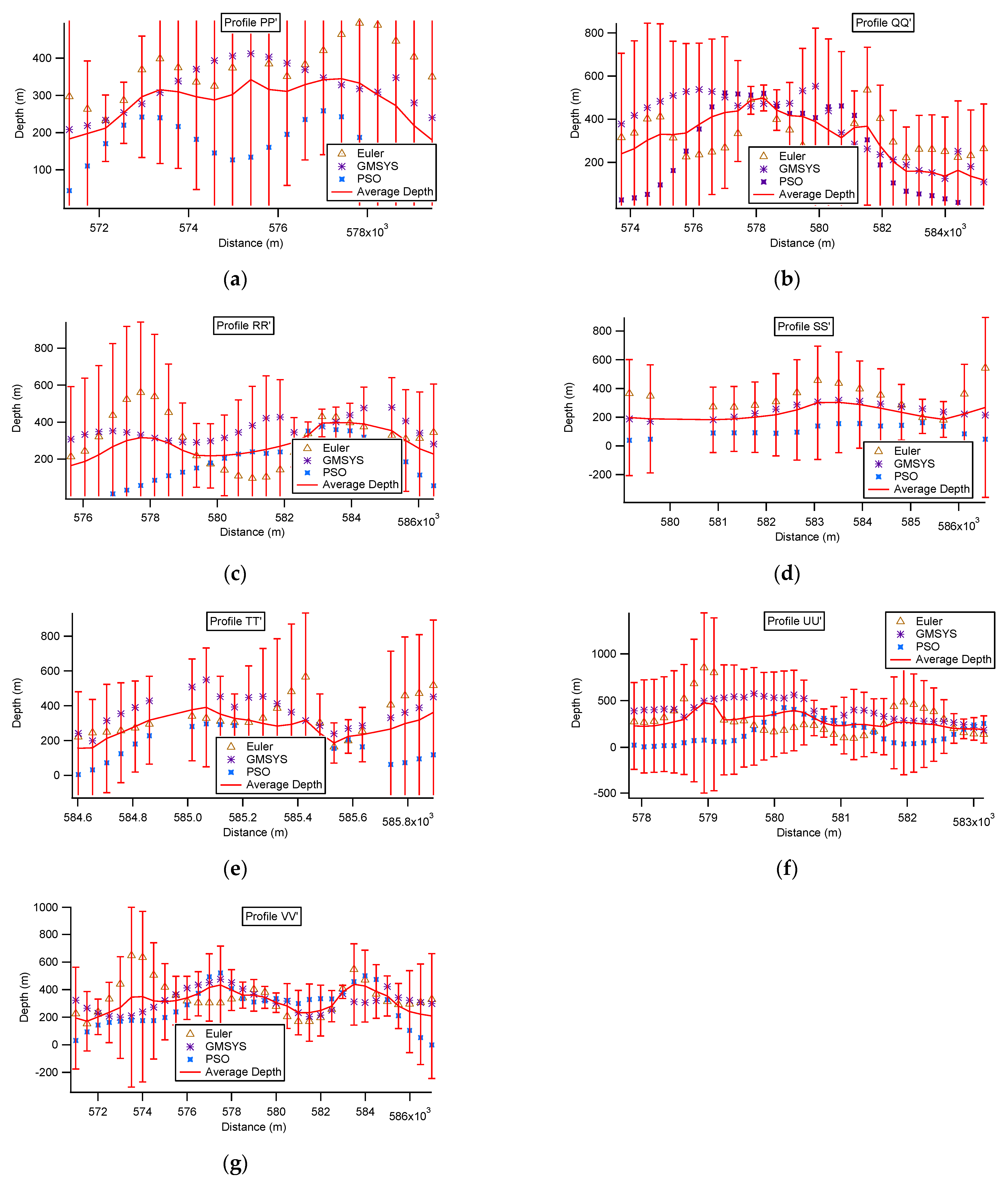
| Profile | Longitude (°) | Latitude (°) | Length (km) | Azimuth (°) |
|---|---|---|---|---|
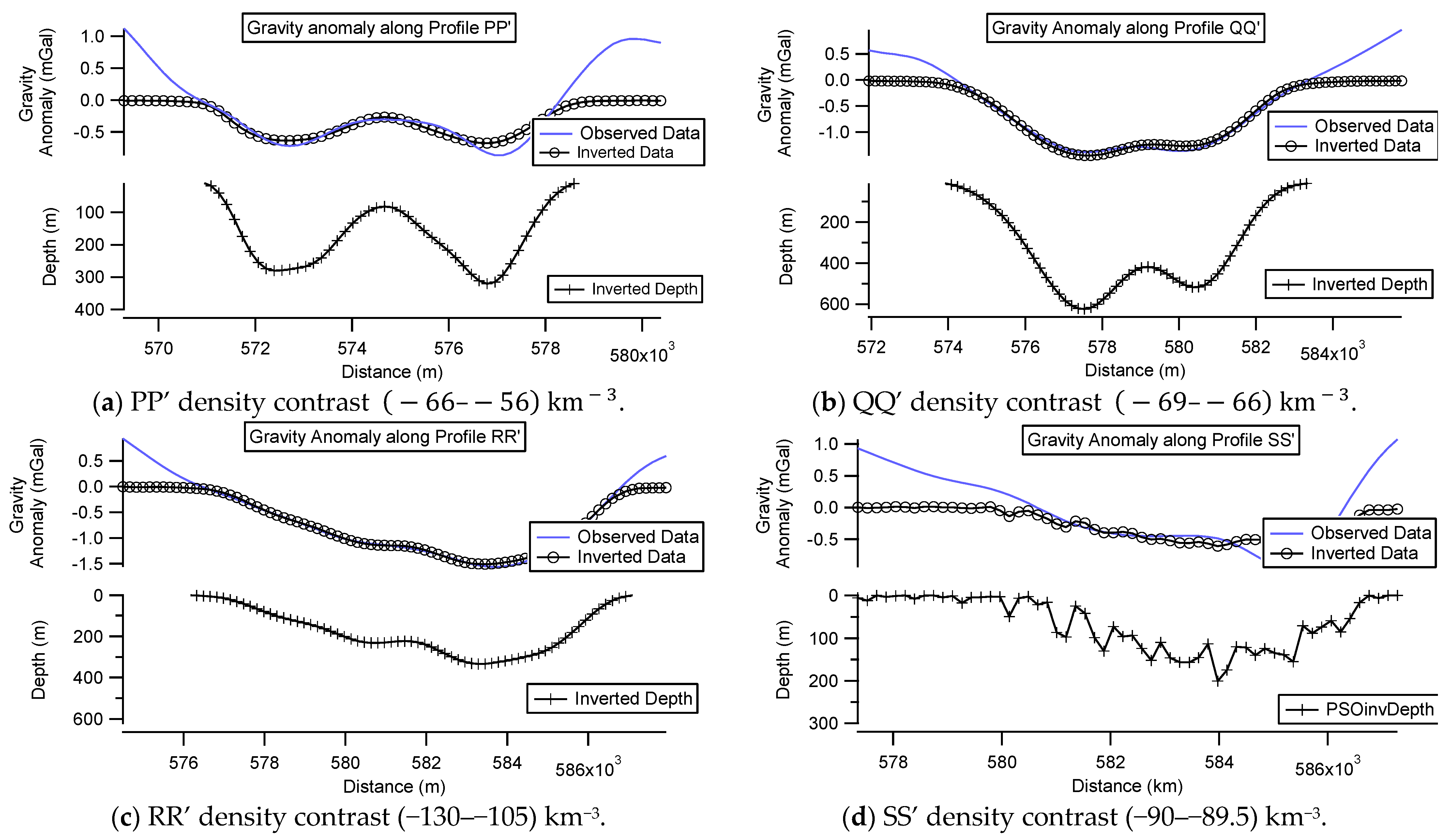
| PP’ | 39.69 39.79 | 24.25 24.18 | 12.74 | 144.3 |
| QQ’ | 39.71 39.85 | 24.28 24.20 | 16.89 | 145.6 |
| RR’ | 39.74 39.87 | 24.30 24.22 | 16.35 | 145.8 |
| SS’ | 39.76 39.86 | 24.33 24.27 | 13.52 | 150.4 |
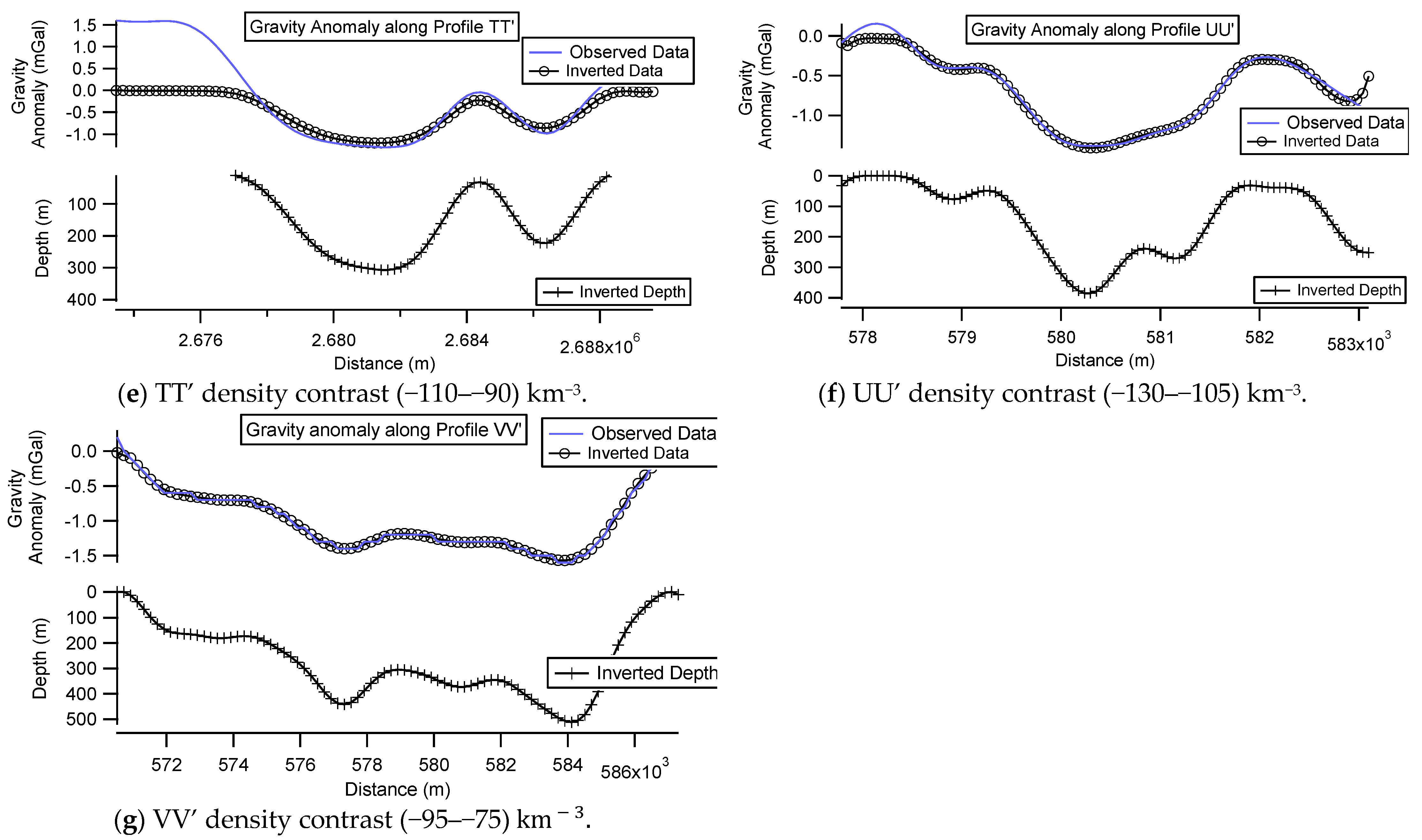
| TT’ | 39.83 39.85 | 24.32 24.16 | 16.37 | 83.1 |
| UU’ | 39.77 39.82 | 24.33 24.16 | 18.13 | 43.5 |
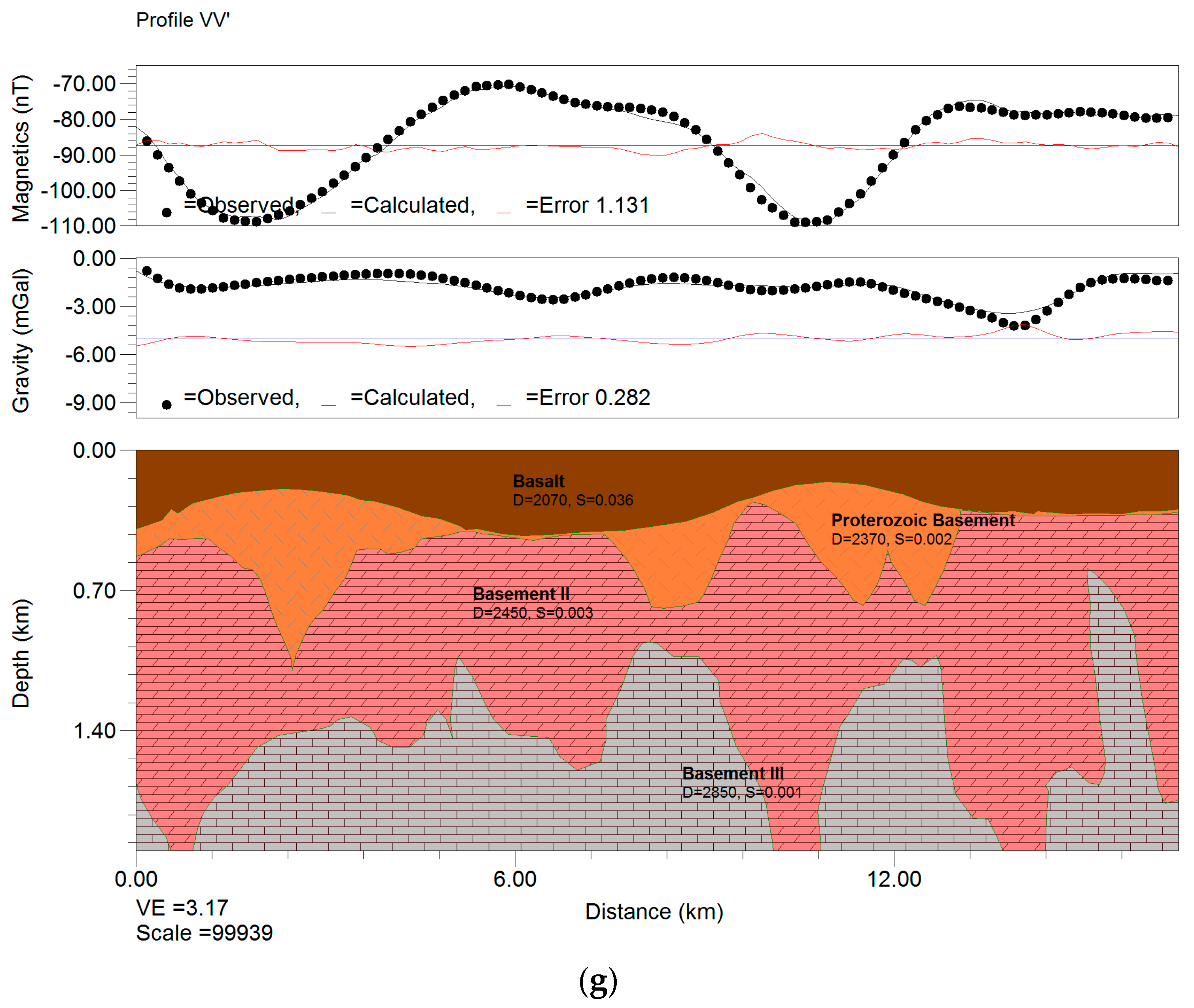
| VV’ | 39.69 39.87 | 24.25 24.25 | 18.53 | 0.1 |
| Profile | No. of Parameters | RMS Error in Gravity Anomaly (mGal) | Depth Range (m) | Mean Depth (m) |
|---|---|---|---|---|
| PP’ | 19 | 0.215391 | 320.59 | 121.29 |
| QQ’ | 12 | 0.130457 | 624.29 | 224.18 |
| RR’ | 12 | 0.098459 | 333.75 | 146.26 |
| SS’ | 99 | 0.212882 | 200.54 | 65.04 |
| TT’ | 11 | 0.241633 | 306.96 | 115.14 |
| UU’ | 14 | 0.046893 | 385.77 | 142.69 |
| VV’ | 18 | 0.033018 | 511.41 | 269.83 |
Publisher’s Note: MDPI stays neutral with regard to jurisdictional claims in published maps and institutional affiliations. |
© 2022 by the authors. Licensee MDPI, Basel, Switzerland. This article is an open access article distributed under the terms and conditions of the Creative Commons Attribution (CC BY) license (https://creativecommons.org/licenses/by/4.0/).
Share and Cite
Alqahtani, F.; Abraham, E.M.; Aboud, E.; Rajab, M. Two-Dimensional Gravity Inversion of Basement Relief for Geothermal Energy Potentials at the Harrat Rahat Volcanic Field, Saudi Arabia, Using Particle Swarm Optimization. Energies 2022, 15, 2887. https://doi.org/10.3390/en15082887
Alqahtani F, Abraham EM, Aboud E, Rajab M. Two-Dimensional Gravity Inversion of Basement Relief for Geothermal Energy Potentials at the Harrat Rahat Volcanic Field, Saudi Arabia, Using Particle Swarm Optimization. Energies. 2022; 15(8):2887. https://doi.org/10.3390/en15082887
Chicago/Turabian StyleAlqahtani, Faisal, Ema Michael Abraham, Essam Aboud, and Murad Rajab. 2022. "Two-Dimensional Gravity Inversion of Basement Relief for Geothermal Energy Potentials at the Harrat Rahat Volcanic Field, Saudi Arabia, Using Particle Swarm Optimization" Energies 15, no. 8: 2887. https://doi.org/10.3390/en15082887