Nested Decomposition Approach for Dispatch Optimization of Large-Scale, Integrated Electricity, Methane and Hydrogen Infrastructures

Abstract

Energy system integration enables raising operational synergies by coupling the energy infrastructures for electricity, methane, and hydrogen. However, this coupling reinforces the infrastructure interdependencies, increasing the need for integrated modeling of these infrastructures. To analyze the cost-efficient, sustainable, and secure dispatch of applied, large-scale energy infrastructures, an extensive and non-linear optimization problem needs to be solved. This paper introduces a nested decomposition approach with three stages. The method enables an integrated and full-year consideration of large-scale multi-energy systems in hourly resolution, taking into account physical laws of power flows in electricity and gas transmission systems as boundary conditions. For this purpose, a zooming technique successively reduces the temporal scope while first increasing the spatial and last the technical resolution. A use case proves the applicability of the presented approach to large-scale energy systems. To this end, the model is applied to an integrated European energy system model with a detailed focus on Germany in a challenging transport situation. The use case demonstrates the temporal, regional, and cross-sectoral interdependencies in the dispatch of integrated energy infrastructures and thus the benefits of the introduced approach.

1. Introduction

1.1. Motivation

In order to achieve greenhouse gas neutrality, energy policies like the Green Deal of the European Commission aim for energy system integration [1]. Besides high energy efficiency, integrated energy systems are characterized by a versatile energy mix that includes molecule-based energy carriers in addition to electricity [2]. These include natural gas transitionally and hydrogen, as well as biogenic and synthetic methane in the long term. Moreover, a coordinated and cross-sectoral operation of the energy infrastructures, hereinafter referred to as integrated energy infrastructures (IEI), is an important property of integrated energy systems [2].

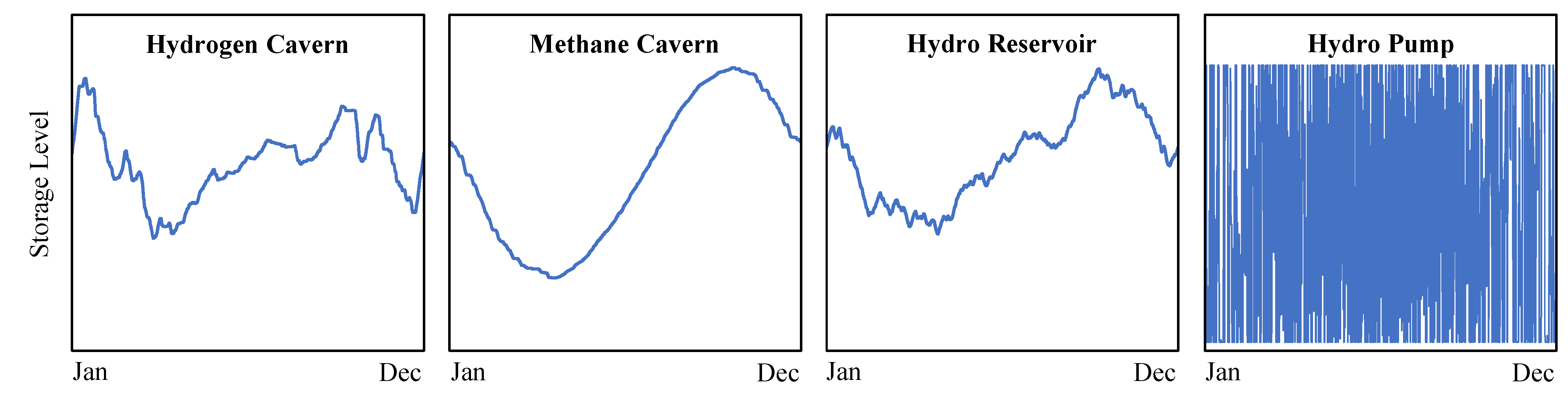
In renewable energy systems, the electricity infrastructure needs to integrate large amounts of intermittent renewable energy sources (RES). This results in high demand for spatial and temporal flexibility in terms of transport as well as short-term and seasonal storage options [3]. A bidirectional coupling with the existing gas infrastructure by gas-fired power plants and power-to-gas plants can provide this flexibility [4]. In addition to the existing natural gas infrastructure, dedicated hydrogen infrastructures are supposed to integrate RES and supply a future hydrogen economy [5].

In order to derive design principles for the future system, a comprehensive understanding of interactions between these infrastructures in operation is required. For example, cost-benefit analyses can be applied to analyze, evaluate, and compare different concepts of IEI. Such analyses require a dispatch simulation in order to determine key indicators such as costs, emissions or energy not served [6,7].

For modeling the dispatch of IEI, different requirements arise. IEI enable raising system-wide synergies to operate the energy system cost-efficiently, sustainably, and securely. However, interdependencies between the coupled infrastructures increase. To adequately address these, an integrated modeling approach rather than a co-simulation approach is necessary [8]. Furthermore, the provision of temporal flexibility by IEI requires the modeling of a full year in at least hourly resolution [9]. Besides temporal resolution, the choice of spatial resolution has a strong impact on the results of energy system modeling [10]. To sufficiently model spatial flexibility, its transmission losses, and operating limits, the physical laws determining the power flows must be considered [8,11]. Finally, the modeling should be applicable to real interconnected energy systems, such as the European energy system to draw application-related conclusions. Thus, the following criteria serve as requirements for this paper:

• Integrated modeling of multi-energy-infrastructures
• Consideration of a full year in at least hourly resolution
• Consideration of transmission systems in nodal resolution and the physical laws determining their power flows (electricity and gas flows)
• Application on real, large-scale energy systems

1.2. Literature Review on Dispatch Models for IEI

In the following, selected models are analyzed with respect to the raised requirements. They either explicitly or implicitly simulate and optimize the dispatch of energy infrastructures. Table 1 provides an overview of selected models. The discussed models consider at least two coupled infrastructures and pursue an integrated modeling approach. This list does not claim to be complete but is intended to provide a broad overview of the literature.

Integrated electricity and gas market models represent a model class of dispatch models that focus on simulating the dispatch of power plants (Unit Commitment and Economic Dispatch) and gas supply [12,13,14,15,16]. Due to present dependencies on district heating systems, these are mostly modeled as additional boundary conditions for dispatch. Market simulations have a high application orientation and are therefore usually applied to real energy systems such as the European or American energy markets [12,14]. These models focus on a full-year consideration with high temporal resolution (1 h or 15 min) as well as a high level of technical detail in the modeling of power plants.

In contrast, the modeling of transmission networks for electricity is often simplified by considering exchange capacities between bidding zones, following the zonal electricity market design [12,13,16]. Transport within a bidding zone is then assumed to be free of congestion. Alternatively, market simulations can model the nodal electricity market design such as the commercial software PLEXOS [16]. PLEXOS applies the DC power flow approximation. In market simulations, the transmission networks for gas are usually modeled with a network flow algorithm with linear transfer capacities neglecting fluid mechanics. Market simulations often apply decomposition approaches such as Lagrange relaxation [17] to solve the resulting linear (LP) or mixed-integer problem (MIP) [13,16].

Investment models have similar qualities to market simulations since this model class needs to model the system dispatch to adequately derive investment decisions. In contrast to market simulations, investment models inherently consider the energy system as a whole, so that interactions between all relevant energy carriers are taken into account. In addition to aggregation in the spatial dimension, investment models such as DIMENSION+ [18], REMod-D [19], IKARUS [20], and PRIMES [21] often aggregate in the temporal dimension to extrapolate the operating costs from type days or weeks. Other investment models like TIMES [22], REMix [23,24], and PyPSA [25] increase their spatial resolution by modeling smaller regions or even network nodes and applying a DC power flow (see next paragraph) between its interconnectors. Nemec-Begluk [26] develops a nested decomposition approach that allows modeling the transmission grid in nodal resolution with a DC power flow. Subsequent to the investment decisions, the total period is sliced into smaller sections. Again, gas infrastructures are not physically modeled in these approaches. Nonetheless, REMix uses a more detailed representation of the gas infrastructure compared to other investment models. It considers additional operational aspects of gas infrastructure dispatch such as estimations for driving energy of compressors [24].

Optimal power and gas flow models (OPGF) represent a class of dispatch models, which model the physical laws of power and gas flows in detail. Thus, they consider the physical potentials voltage and pressure. Since the integrated operation of the networks also includes the dispatch of conversion plants such as power-to-gas plants or gas-fired power plants, these models often optimize the dispatch of these plants in addition to network optimization. For these models, modeling the non-linear physical laws resulting from power and gas flows is the main challenge. The AC power flow equations describe the trigonometric and quadratic dependence of active and reactive power flow from voltage magnitude and phase angle. By assuming flat voltage profiles, small voltage angle differences and small resistance to reactance ratios (R/X), linear dependencies arise for modeling the active power flow [27]. This so-called DC power flow approximation is a permissible and common simplification for planning issues at transmission grid level [11]. Gas flows are determined by fluid mechanics and described by three differential equations for mass, momentum, and energy conservation [8]. Thus, transient modeling of dynamic gas flows requires high spatial and temporal resolution. Complexity can be reduced by assuming steady-state conditions, which is a common simplification for planning issues of gas transmission networks [28]. However, this still results in a non-linear system of equations [29]. Under so called quasi-steady-state conditions, slow dynamics of mass conservation of gases and linepack flexibility can be simplified considered in hourly resolution [29,30,31,32].

The commercial software SAInt [8,33] provides an integrated modeling approach with AC power flows and transient gas flows. Source [30,34] also model the physical flows in detail. Other approaches like [31,35,36,37,38,39] apply the DC power flow approximation as well as steady-state gas flow assumptions to reduce the complexity of the OPGF problem. Sources [29,30,31,32] consider simplified gas dynamics by using a quasi-steady-state formulation. The non-linear optimization problem is often solved by applying piecewise linearization approaches like in [35,38,39] or non-linear solvers like in [30,34,37]. The resulting problem is often applied to small test systems and periods of usually 24 h since these approaches are difficult to scale up for large problem sizes [29]. Chaudry et al. [36] solve the OPGF problem for large-scale systems and 24 h using a commercial solver based on successive linear programming (SLP). However, they also address problems with further scalability. Löhr et al. [29] introduce a SLP-based approach showing good scaling properties. It is applied to a power and gas transmission system with over 500 nodes each for a 24 h period.

The OPGF problem commonly considers the electricity and natural gas infrastructure. A bidirectional coupling of electricity and gas infrastructure is a comparatively new aspect. Therefore, power-to-gas plants are only modeled in [29,30,33]. Schwele et al. [40] additionally consider heat infrastructures with physical thermal power flows. Hydrogen transport grids are a new research topic in energy system analysis and are not considered explicitly in the presented literature. The Energy Hub Concept by Geidl [41,42] basically allows modeling any number of infrastructures and conversion processes between different energy carriers as well as AC power and steady-state gas flows.

Therefore, this literature review shows a research gap. On the one hand, there are energy system models, that can be applied for long periods and large-scale systems but have a low spatial and technical resolution when modeling transmission infrastructures. On the other hand, there are models with high spatial and technical detail, but can only be applied to short periods and small systems. Thus, to the best of the author’s knowledge, no model that meets all listed requirements for dispatch simulation of IEI exists.

Table 1. Overview of selected existing dispatch models for integrated energy infrastructures.

References	Name	Model Class	Energy Carrier	Physics Power/Gas	Spatial Scope/Resolution	Temporal Scope/Resolution
[12]	Riepin et al.	Market	electricity, gas	network flow	Europe/country	year/1 h
[13]	Baumann	Market	electricity, gas	network flow	Europe/country	year/1 h (1 d)
[14,15]	Quelhas et al.	Market	electricity, gas, coal	network flow	USA/US regions	year/1 h
[16]	PLEXOS	Market	electricity, gas, heat	DC/network flow	USA/Europe/nodal	year/(≥1 min)
[21]	PRIMES	Invest	total energy system	DC/network flow	Europe /country	years/1 h (type)
[23,24]	REMix	Invest	total energy system	DC/network flow	Germany/regions	years/1 h
[25]	PyPSA	Invest	total energy system	DC/network flow	Europe/nodal	years/1 h
[26]	Nemec-Begluk	Invest	electricity, gas, heat	DC/network flow	Austria/nodal	year/1 h
[41,42]	Geidl	OPGF	all (modular)	AC/steady state	3 × 3 test/nodal	day/1 h
[38]	Correa-P. et al.	OPGF	electricity, gas	DC/steady state	24 × 20 test/nodal	day/1 h
[30]	Sun et al.	OPGF	electricity, gas	AC/q.-steady state	24 × 20 test/nodal	day/1 h
[40]	Schwele et al.	OPGF	electricity, gas, heat	DC/steady state	24 × 12 × 3 test/nodal	day/1 h
[8,33]	SAInt, Pambour	OPGF	electricity, gas	AC/transient	30 × 25 test/nodal	day/1 h
[36]	Chaudry et al.	OPGF	electricity, gas	DC/steady state	16 × 168 UK/nodal	day/1 h
[29]	Löhr et al.	OPGF	electricity, gas	DC/q.-steady state	542 × 524 GER/nodal	day/1 h

Table 1. Overview of selected existing dispatch models for integrated energy infrastructures.

References	Name	Model Class	Energy Carrier	Physics Power/Gas	Spatial Scope/Resolution	Temporal Scope/Resolution
[12]	Riepin et al.	Market	electricity, gas	network flow	Europe/country	year/1 h
[13]	Baumann	Market	electricity, gas	network flow	Europe/country	year/1 h (1 d)
[14,15]	Quelhas et al.	Market	electricity, gas, coal	network flow	USA/US regions	year/1 h
[16]	PLEXOS	Market	electricity, gas, heat	DC/network flow	USA/Europe/nodal	year/(≥1 min)
[21]	PRIMES	Invest	total energy system	DC/network flow	Europe /country	years/1 h (type)
[23,24]	REMix	Invest	total energy system	DC/network flow	Germany/regions	years/1 h
[25]	PyPSA	Invest	total energy system	DC/network flow	Europe/nodal	years/1 h
[26]	Nemec-Begluk	Invest	electricity, gas, heat	DC/network flow	Austria/nodal	year/1 h
[41,42]	Geidl	OPGF	all (modular)	AC/steady state	3 × 3 test/nodal	day/1 h
[38]	Correa-P. et al.	OPGF	electricity, gas	DC/steady state	24 × 20 test/nodal	day/1 h
[30]	Sun et al.	OPGF	electricity, gas	AC/q.-steady state	24 × 20 test/nodal	day/1 h
[40]	Schwele et al.	OPGF	electricity, gas, heat	DC/steady state	24 × 12 × 3 test/nodal	day/1 h
[8,33]	SAInt, Pambour	OPGF	electricity, gas	AC/transient	30 × 25 test/nodal	day/1 h
[36]	Chaudry et al.	OPGF	electricity, gas	DC/steady state	16 × 168 UK/nodal	day/1 h
[29]	Löhr et al.	OPGF	electricity, gas	DC/q.-steady state	542 × 524 GER/nodal	day/1 h

1.3. Contribution and Paper Organization

Hence, the purpose of this paper is to introduce a method that enables dispatch modeling for IEI meeting the requirements listed in Section 1.1. The novelty of this method is the combined capability of modeling non-linear physical power and gas flows while allowing applicability to large-scale systems and long periods.

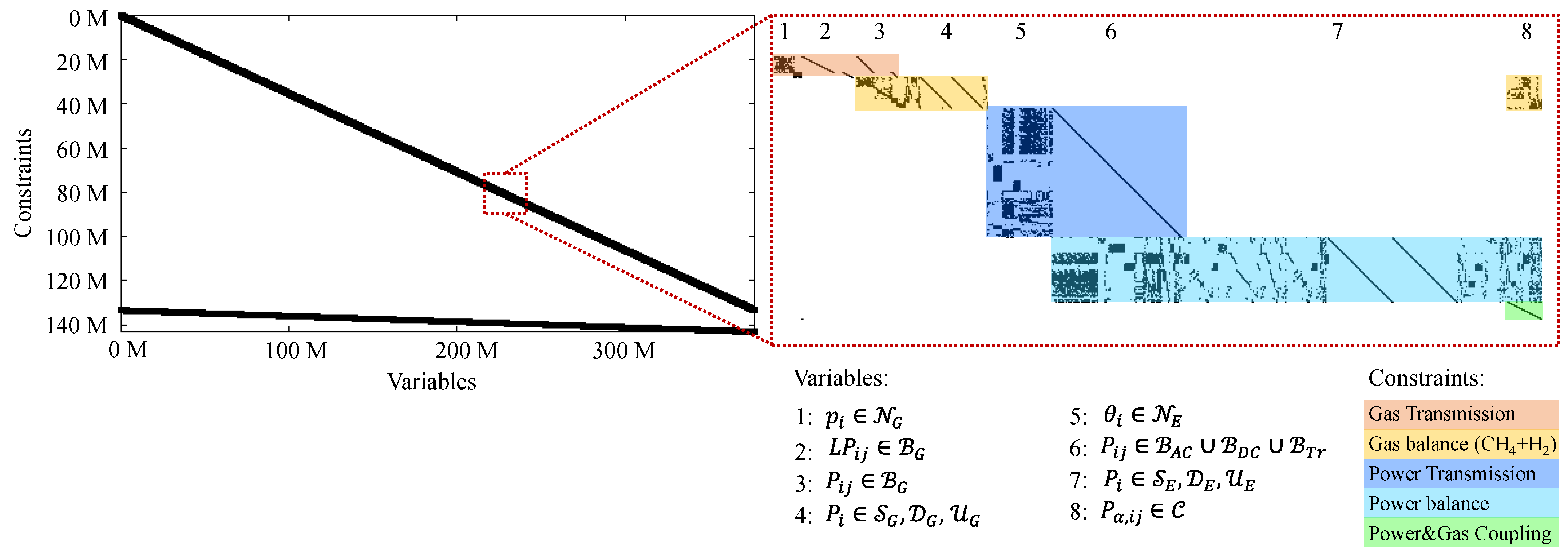
The introduced model is based on an integrated optimization approach that models electricity, methane, and hydrogen infrastructures “as a whole” integrated energy infrastructure. A DC-power flow and a quasi-steady-state gas flow formulation allow detailed analyses of IEI on grid node level. Thus, network bottlenecks and transport losses can be determined and the temporal flexibility of gas infrastructures through linepacking can be considered. The basic optimization problem describing the dispatch problem for IEI is formulated in Appendix A.

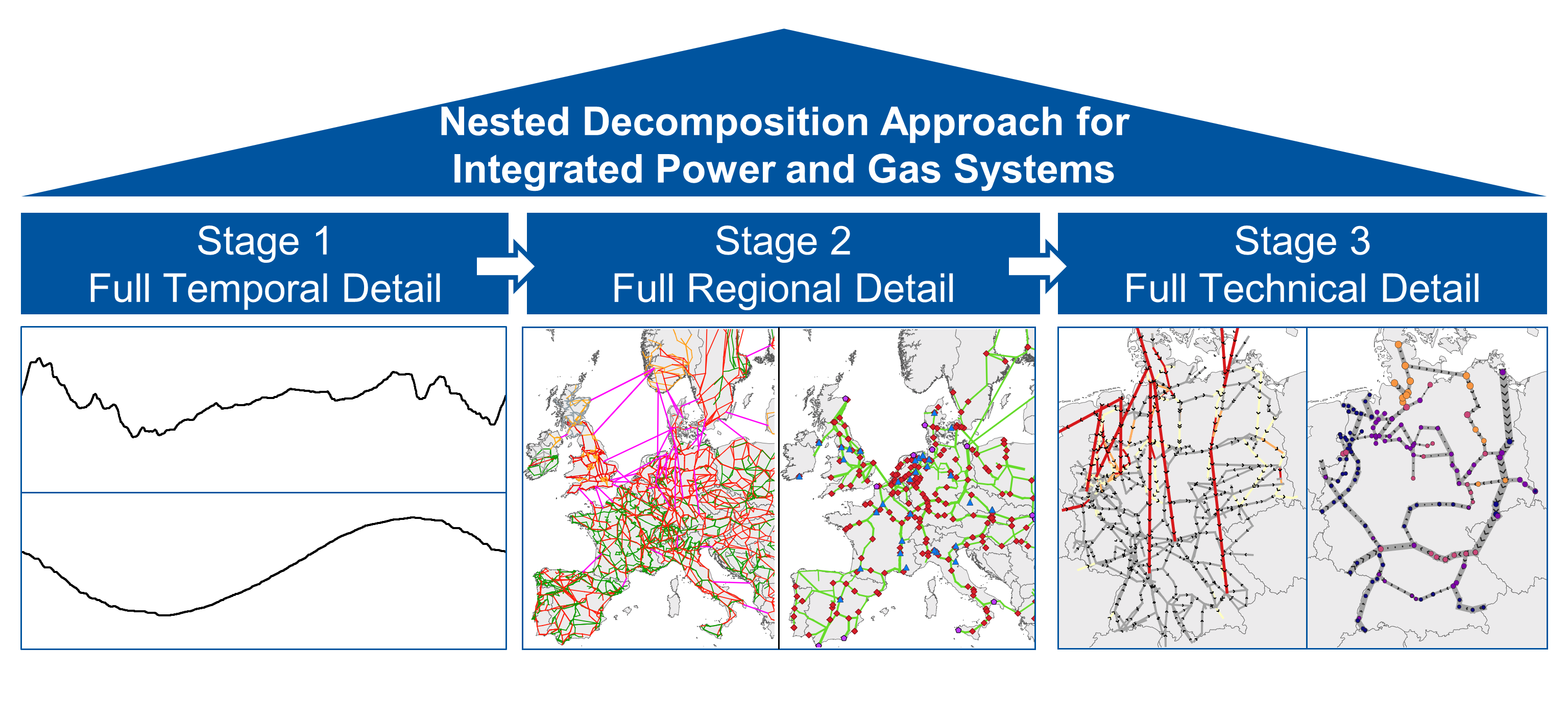
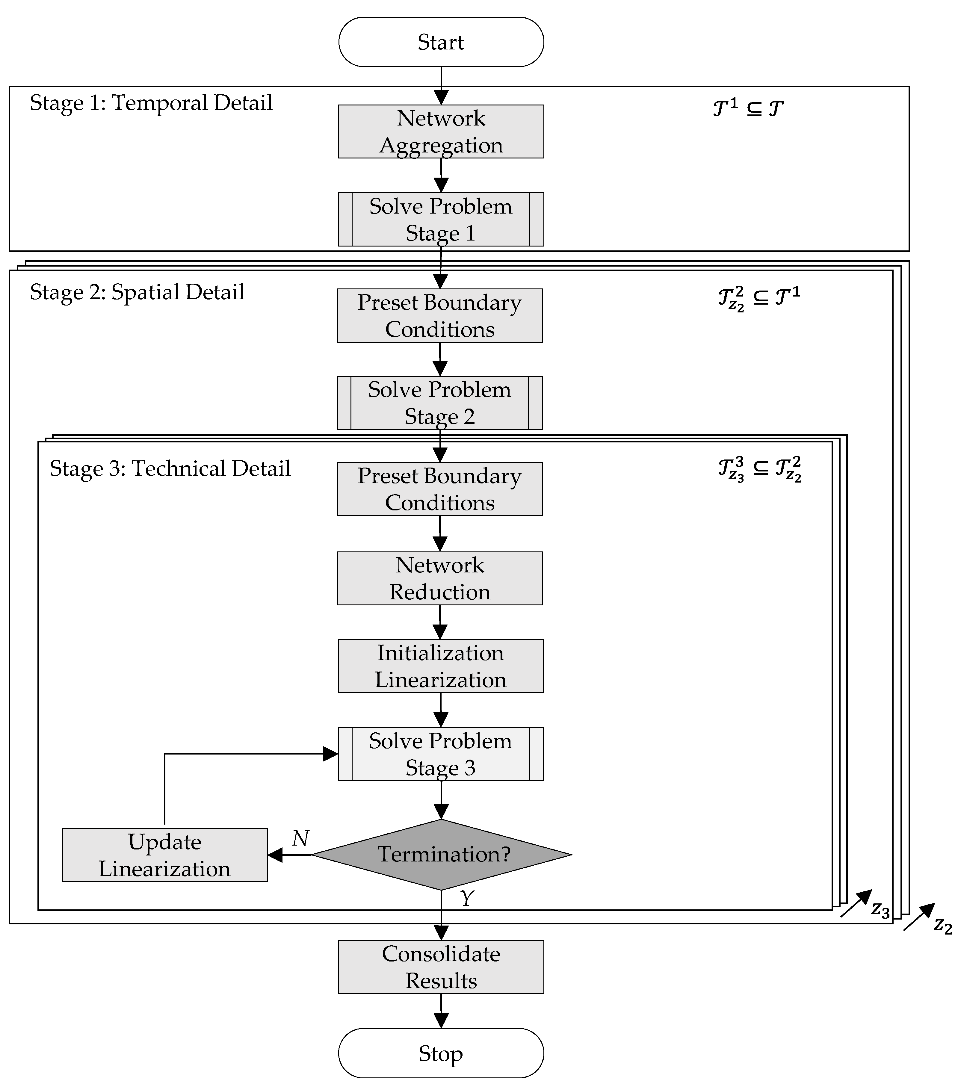
These specifications result in a complex mathematical problem, that cannot be solved in a closed-loop optimization with currently available solvers and resources. To enable this level of detail, various model reduction and decomposition techniques are applied. The approach of this paper builds on the SLP-based OPGF model introduced in [29]. This model is integrated into a three-staged nested heuristic. The nested decomposition approach applies successive zooming techniques that focus first on the temporal, then on the spatial, and finally on the technical dimension. Complexity is handled by model reductions of the other dimensions in each stage, which enables scalability to an entire year in hourly resolution and large-scale systems in high technical detail. The main contribution of this paper is to demonstrate the combined application of several model reduction and decomposition techniques to handle application-oriented, large-scale problems. Therefore, it focuses on the methodology presented in Section 2.

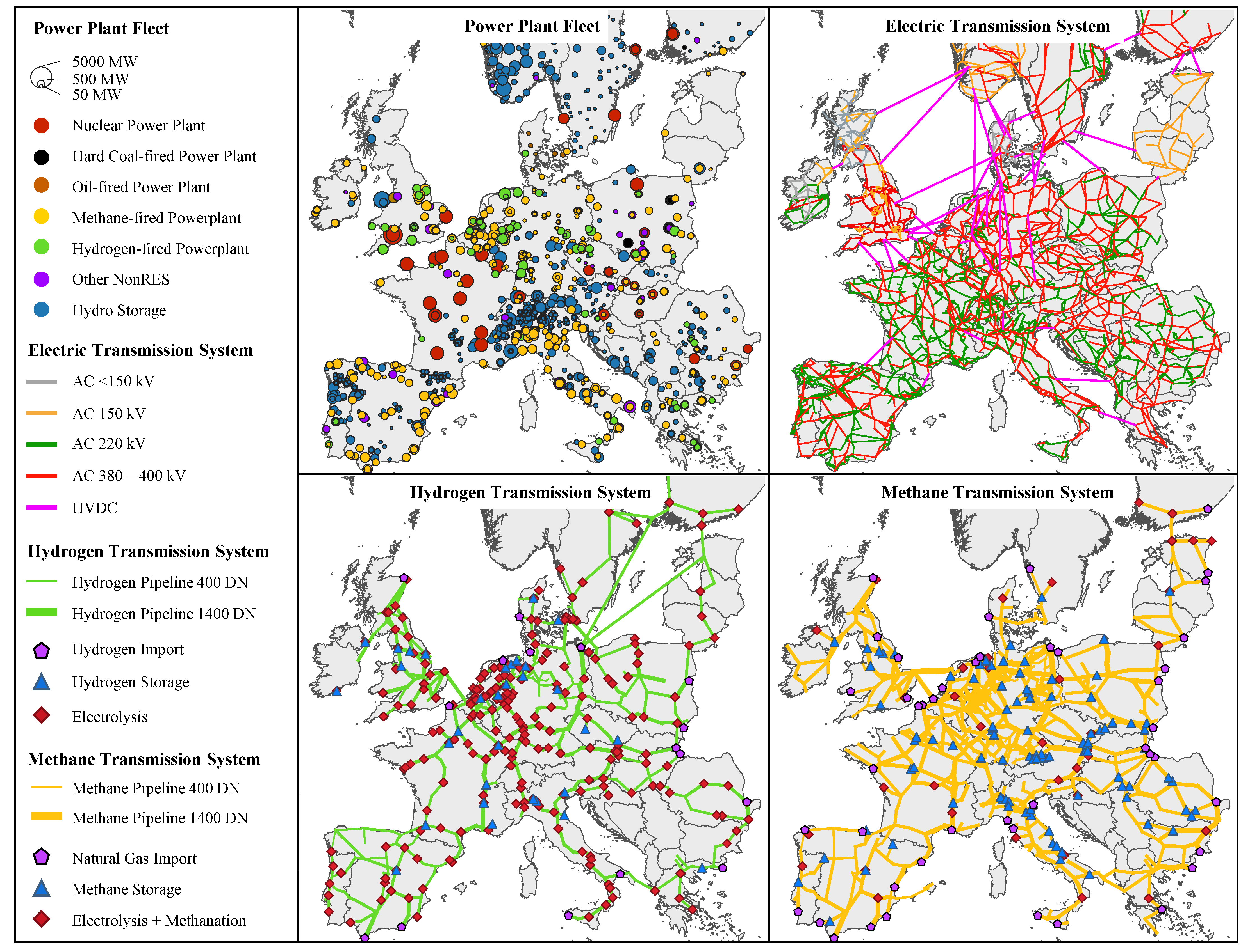
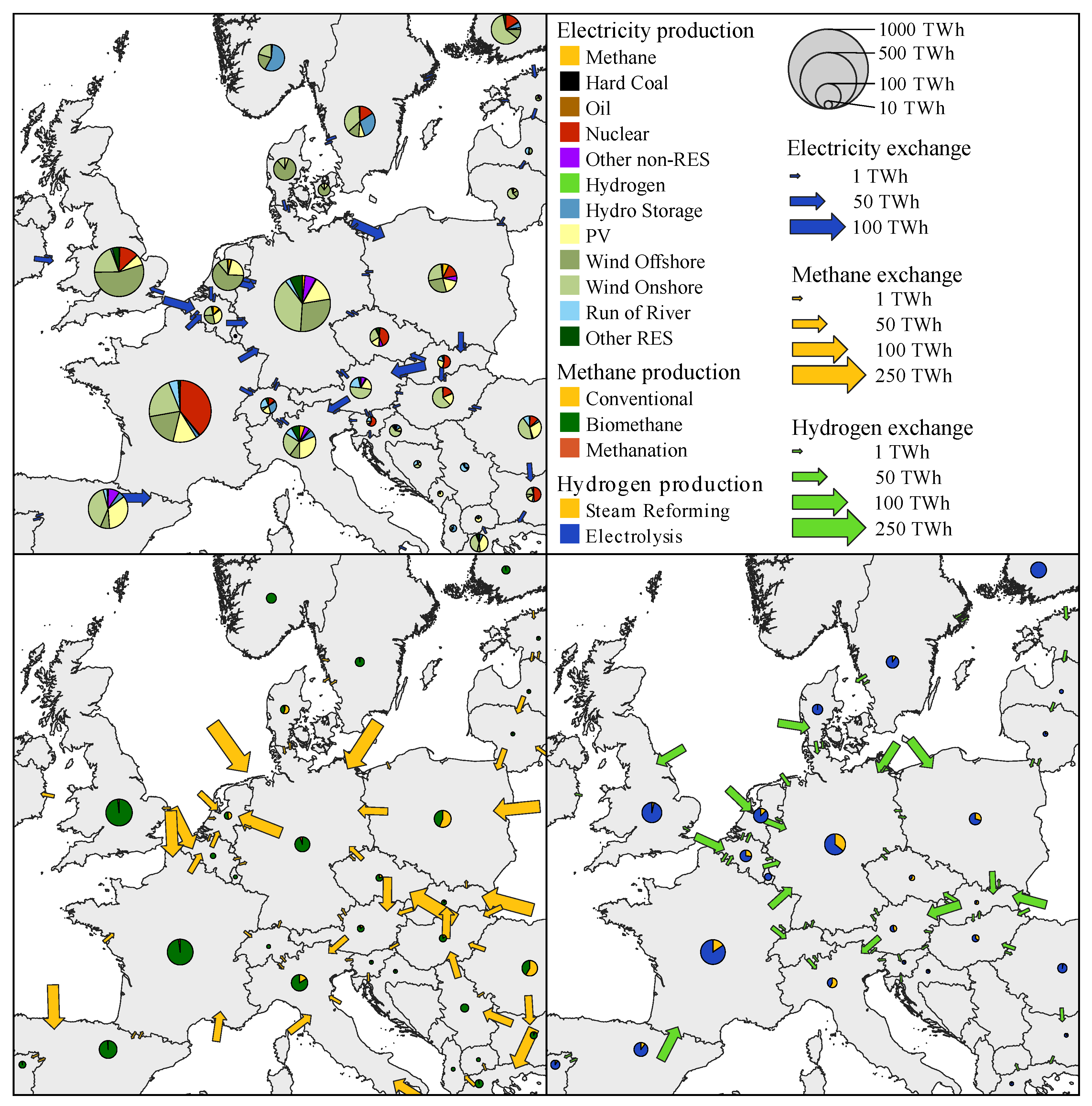
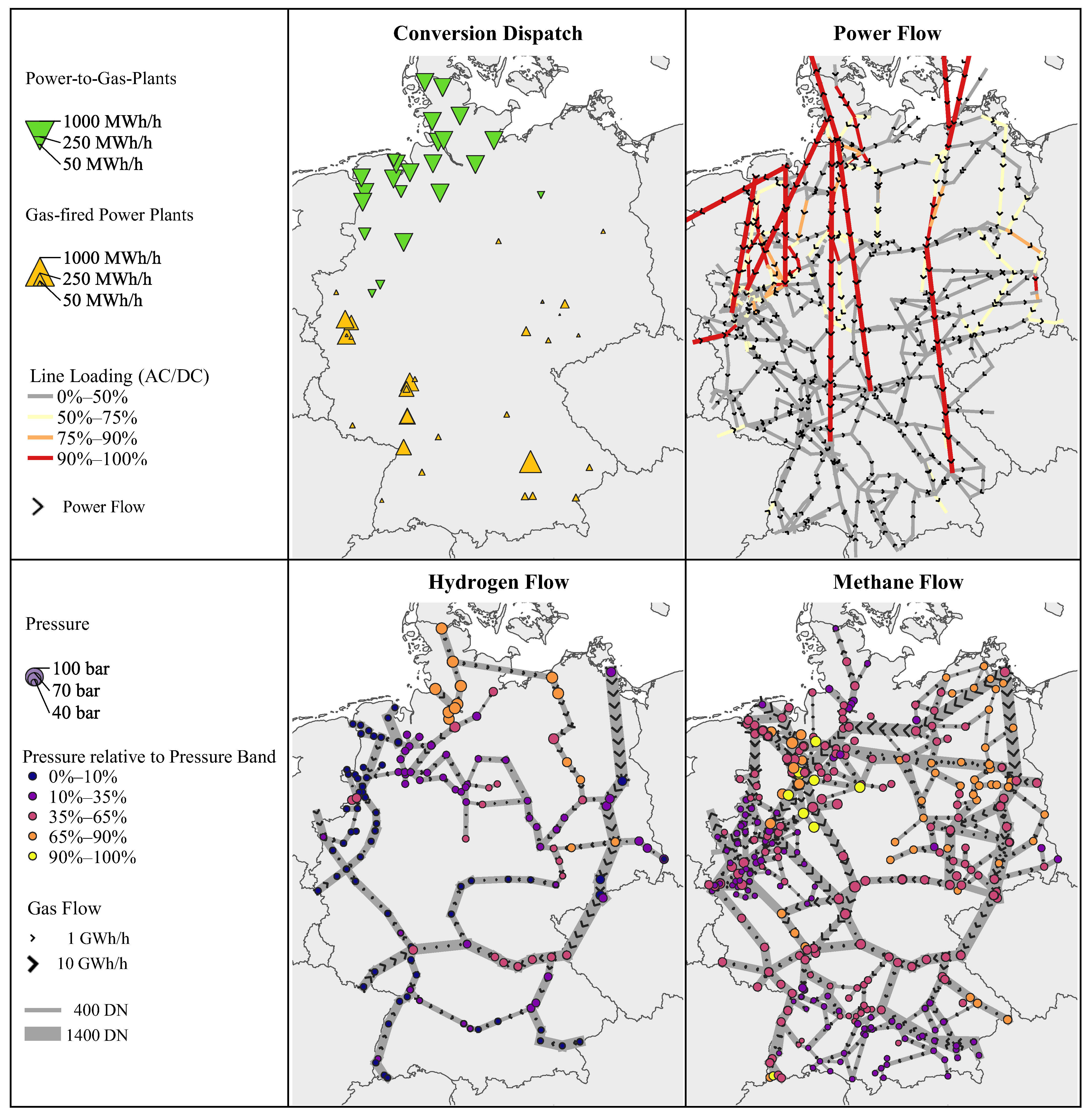
The closing investigations in Section 3 are intended to prove the applicability of the approach to large-scale systems and illustrate the temporal, spatial, and cross-sectoral interdependencies in IEI and therefore the benefits of the introduced approach. For this purpose, a use case of the future interconnected European energy system in 2040 with a focused analysis of the dispatch in Germany is considered. Application-oriented analyses of European energy infrastructure with the presented spatial, temporal, and technical scope also represent a novelty. Section 4 concludes the main findings of this paper.

2. Nested Decomposition Approach

2.1. Integrated Dispatch Optimization Problem

The nested decomposition approach is based on an integrated dispatch optimization problem. For reasons of clarity, this is only briefly characterized in this section and is presented mathematically in Appendix A.

The dispatch optimization problem considers the energy infrastructure in an integrated manner as a coherent graph for the energy carrier electricity (AC and DC), hydrogen, and methane. The nodes of the IEI graph describe busbars and gas stations. Branches either connect two nodes within an infrastructure or connect two infrastructures with each other (conversion plants). In the power system, branches represent AC lines, DC lines, and (phase-shifting) transformers. In the infrastructures for gases, branches model pipelines, compressors, and pressure regulating valves. The considered conversion plants are electrolyzers, gas-fired power plants, fuel cells, steam methane reforming, and methanation plants. Power and gas storage, as well as other feed-in and feed-out plants, are connected to nodes. Degrees of freedom of other feed-in and feed-out plants is the dispatch of power plants, gas imports, RES curtailment, or demand-side response (DSR).

The objective (A25) of the optimization is to minimize dispatch costs. These are in particular fuel costs, costs for DSR, and costs for loss of load (energy not served). Perfect foresight is assumed. The following constraints must be considered when dispatching the system:

• Node balance equation in each infrastructure (A1)
• DC power flow Equations (A3) and (A5)
• Electrical transmission loss Equation (non-linear) (A6)
• Steady-state pressure loss Equation (non-linear) (A7)
• Linepack Equations (non-linear) (A8)–(A11)
• Horsepower equations for losses in compression (non-linear) (A16)–(A18)
• Conversion continuity Equation (A19)
• Storage continuity Equation (A20)
• Technical operation limits in Equations (A2), (A4), (A12)–(A15), (A21)–(A24)

The resulting OPGF problem thus uses the DC load flow approximation including transmission losses and a quasi-steady state gas flow formulation. The formulated optimization problem has a linear objective function, linear and non-linear constraints, and no integer variables.

2.2. Analysis of Complexity Drivers

In energy system modeling, complexity can result due to various drivers in technological, temporal, and spatial dimension [43]. One driver is the pure size of the problem, which results from considering multiple infrastructures, large-scale systems, or large periods [44]. Linking variables and constraints, which increase dependencies between different technologies, regions, and time steps, make it difficult to decompose the problem [43]. Another complexity driver results from non-linear and integer relations, which make the problem harder and complicate the application of efficient algorithms [43,45].

The formulated dispatch optimization problem already avoids some complexity drivers such as integer decisions and non-linear objective functions. Nevertheless, non-linear constraints remain to model the hydraulic gas flows, linepack, compressors, as well as electrical losses. Moreover, the problem is extensive for large network sizes and periods. If the stated problem is applied to the European scenario in Section 3, this results in nearly 400 million variables and over 140 million constraints. Among them are several linking constraints. The population of the coefficient matrix is suitable to identify and visualize the structure of the optimization problem and its linking constraints [43,44]. Figure 1 shows the population of the coefficient matrix of the linearized integrated dispatch problem in full technical detail (see Section 2.7) when applied to the European scenario.

The coefficient matrix shows at the top a diagonal block structure, which is typical for energy system models [44]. A block represents a discrete time step $t\in \mathcal{T}$, that consists of constraints for nodal balances and physical transport for electricity and gases, respectively. In addition, a block contains coupling constraints between the infrastructures. Electrical or thermal power flows on the lines is included in both the transport constraints and the nodal balance. In contrast, physical potentials and linepack variables are only incorporated into the transport equations, feed-ins, and feed-outs only into the nodal balance. Conversion plants are an exception as they are additionally present in coupling constraints. These constraints represent spatial and technological linking constraints. Temporal linking constraints, which result from storages and linepack, form a second diagonal at the bottom of the matrix. These connect variables of different blocks with each other.

2.3. Overview on Model Reduction and Decomposition Techniques

Various techniques exist for reducing modeling complexity. First, model reduction techniques are briefly introduced. According to [46], model reduction techniques can be subdivided into techniques of slicing and aggregation in the dimensions of time, space, and technology. Slicing approaches consider a subproblem of the original problem, reducing its scope and neglecting interactions between subproblems. Slicing is especially effective to decompose linking constraints and variables. In contrast, aggregation approaches reduce the model detail while keeping the full scope of the problem. Among others, aggregation can be useful to relax non-linear or integer relations.

Table 2. Model reduction techniques based on [46].

Dimension	Slicing	Aggregation
Time	Division of periods in subperiods Analysis of type-hours/days/weeks	Down sampling temporal resolution
Space	Neglection of peripheral systems Decoupling of interconnected systems	Clustering of network nodes Network reduction algorithms
Technology	Neglection of technologies and infrastructures	Merging single plants to classes Simplified models (e.g., linearization)

presents an overview of common model reduction techniques.

Accordingly, slicing narrows the scope of the problem, for example by considering subperiods or subregions and neglecting whole infrastructures or technologies. Aggregation reduces temporal or spatial granularity and simplifies technological models. Network reduction algorithms such as the Ward-method for power systems represent an example of spatial aggregation [47]. This method aims to reduce network nodes in peripheral areas while still representing the physical power flows within the focus area. For this purpose, suitable virtual lines and feed-in/outs that correspond to the electrical behavior of the peripheral area are determined. The simplified physical power and gas flow formulations introduced in Section 1.2 represent technical aggregation methods.

According to the principle “divide and conquer”, decomposition techniques intend to make model size and complexity manageable by dividing the problem. A distinction can be made between mathematically exact methods and heuristic approaches [46]. Mathematically exact methods reformulate the problem and solve it in an iterative process. Examples are the Dantzig-Wolfe—or the Benders Decomposition, which divides the problem into one main and (various) sub-problems [48,49]. Lagrange Relaxation transfers linking constraints into the objective function [17]. Lagrange Relaxation and Dantzig-Wolfe Decomposition are commonly used to deal with linking constraints, whereas Benders Decomposition is more promising to reduce computation time dealing with linking variables. While these methods maintain the guarantee for optimality, they are also not applicable to large-scale problems with heterogeneous complexity drivers, such as those resulting from the stated requirements. In contrast, heuristic approaches such as nested decomposition approaches can be specifically designed to find a near-optimal, but not guaranteed optimal, solution for an individual problem [46]. However, such a solution may be sufficient for the purpose of energy system analysis. In nested decomposition approaches, the problem is sequentially and coordinately solved multiple times by applying different model reduction techniques in each stage [46]. The solutions of each stage can serve as boundary conditions for the subsequent stages. Zooming techniques represent an example of nested decomposition approaches. Thereby, wide scopes are first modeled in low resolution to afterward model subsections in greater detail. The interactions between the subsections are transferred from the previous stages. Zooming techniques are often applied in temporal dimensions [44] but can also be applied in spatial or technological dimensions. For a detailed description of reduction and decomposition techniques, please refer to [43,44,46].

2.4. Applied Model Reduction and Decomposition Techniques

The developed nested approach primarily decomposes the optimization problem in the temporal dimension due to the shown structure of the coefficient matrix. It applies a zooming technique, where first the total period is considered by performing model reductions in technical and spatial dimension. In two following stages, the technical and spatial level of detail is increased successively by slicing the total period into smaller subperiods. This approach enables parallel computing, resulting in advantages in computation time.

Table 3. Applied model reduction techniques.

Dimension	Stage 1	Stage 2	Stage 3
Time		Slicing to subperiods	Further slicing in subperiods
Space	Aggregation on country level		Aggregation by network reduction
Technology	Aggregation to plant classes Aggregation to network flow (power and gas)	Aggregation to network flow (gas)

summarizes the model reduction techniques of the three stages applied. Figure 2 gives a schematic overview of the nested decomposition approach. In the following, the three stages are described in detail.

2.5. Stage 1: Storage Level Optimization in Full Temporal Detail

The first stage aims to adequately model the dispatch of seasonal storage for electricity and gases. Thus, the focus of this stage is on the temporal dimension. It considers a full year ${\mathcal{T}}_1=\mathcal{T}$ in hourly resolution. To solve this large-scale optimization problem, nodes are aggregated in the spatial dimension to defined regions $ℛ$ (“Network Aggregation”). In this paper, regions are defined at the country level. This aggregation is done for all electricity nodes and gas nodes of each gas type in one region. Further model reductions are applied in the technical dimension. On the one hand, physical laws for power and gas flows are neglected. Instead, the exchange between regions is modeled using a network flow algorithm and network losses are roughly estimated as additional feed-out depending on the residual load of each region. Thus, Equations (A3)–(A18) are not considered in this stage. Exchange capacities result from aggregating interconnector capacities. In the power system, only 70% of the (already reduced) transport capacity of each line is considered as exchange capacity to account for loop flows. Capacities in gas networks are estimated depending on the pipe geometry (pipe length $l$ and diameter $d$), maximum velocity $w_{max}$ and heating value $h_u$ of the gas. The thermodynamic state of the gas such as the compressibility factor $K$ is estimated based on nominal quantities such as the rated pressure $p_N$ of the pipeline.

$$P_{G,ij}^{max}=\frac{p_N}{p_n}·\frac{T_n}{T_m}·\frac{1}{K_m}·w_{max}·\frac{\pi }{4}·d^2·h_u$$

(1)

On the other hand, plants such as power plants or conversion plants are aggregated into plant classes to further reduce complexity. Storages are an exception to this principle. All model reductions result in a linear optimization problem that can be solved in manageable computing time (“Solve Problem Stage 1”).

2.6. Stage 2: Simplified Dispatch Optimization in Full Spatial Detail

The objective of the second stage is still a linear but more detailed estimation of the dispatch of IEI compared to stage 1. Stage 2 derives further constraints for the subsequent final dispatch optimization. Full complexity in spatial and higher complexity in technical dimensions is enabled by slicing the total period $\mathcal{T}$ into subperiods ${\mathcal{T}}_z^2$. An applicable period duration in stage 2 is 168 h (1 week).

$$\underset{z_2\in {\mathcal{Z}}^2}{{\displaystyle \cup }}{\mathcal{T}}_{z_2}^2={\mathcal{T}}^{},\underset{z_2\in {\mathcal{Z}}^2}{{\displaystyle \cap }}{\mathcal{T}}_{z_2}^2=\varnothing$$

(2)

The target storage level at the beginning and end of a sub-period is transferred from the first stage solution (“Preset Boundary Conditions”). This maintains the information about the total period dispatch of storage. In stage 2, all plants are modeled individually, and the transport networks are considered on a nodal level in all defined regions $ℛ$. The DC power flow approximation is applied in the electricity network. In the gas network, a network flow under consideration of (1) is still assumed. Again, electric network losses are estimated as additional feed-outs. Thus, Equations (A6)–(A18) are not considered in this stage. The resulting linear optimization problem is solved (“Solve Problem Stage 2”).

2.7. Stage 3: Dispatch Optimization in Full Technical Detail

The third stage identifies the final dispatch considering the full detail of the formulated optimization problem in Appendix A. To allow this level of detail, model reductions must be made in other dimensions. In the temporal dimension, the subperiods of the second stage are further divided. An applicable period duration in stage 3 is 24 h (1 day).

$$\underset{z_3\in {\mathcal{Z}}^3}{{\displaystyle \cup }}{\mathcal{T}}_{z_3}^3={\mathcal{T}}^{}, \underset{z_3\in {\mathcal{Z}}^3}{{\displaystyle \cap }}{\mathcal{T}}_{z_3}^3=\varnothing$$

(3)

In spatial dimension, the considered regions are divided into focus regions ${ℛ}_{focus}\subseteq ℛ$ and external regions ${ℛ}_{ex}\subseteq ℛ$. The dispatch of plants in external regions is captured from the second stage. Thus, the exchange with the focus area serves as a boundary condition. In addition, storage levels at the beginning and end of a sub-period are transferred from stage 2 solution (“Preset Boundary Conditions”). A network reduction is performed around the focus area (“Network Reduction”). In the electricity network, the Ward method is applied to reduce external nodes but maintain the electric behavior of the network in the focus area. In contrast, hydraulic interdependencies with the external system are neglected in the gas network, since gas flows can be dispatched well by controllers. The full technical model scope is considered in the focus region. This includes in particular the consideration of physical gas flows, electric network losses, and linepack in addition to the DC power flow. Thus, the conservation of mass in the gas network is considered within the periods. Since the time-coupled constraints of the linepack are of short-term nature, dependencies between subperiods are neglected to reduce complexity. The resulting non-linear optimization problem is solved using the successive linearization approach introduced and validated in [29]. In the focus region, the results from stage 2 serve as starting solution for the SLP algorithm (“Initialize Linearization”). The problem is solved successively (“Solve Problem Stage 3”). In each iteration, the linearization is updated, and the intervals of variable bounds are reduced to achieve convergence of the SLP algorithm (“Update Linearization”). The SLP algorithm is terminated when the linearization error of the pressure losses and electrical losses becomes marginal, and the value of the objective function no longer changes significantly. The results of the nested decomposition approach are consolidated by updating the results from stage 2 by the results from stage 3 in the focus regions (“Consolidate Results”).

3. Application of the Approach

The introduced nested decomposition approach is applied to an integrated European energy system scenario for the year 2040 to demonstrate its applicability to large-scale systems. The European states are defined as regions. In the third stage, Germany is considered a focus region to analyze the operational restrictions for long-distance transport in detail. The problem is calculated for a full year in hourly resolution. Therefore, stage 1 considers 8760 h time coupled. Stage 2 slices the year into weekly periods (~52 × 168 h), stage 3 in daily periods (365 × 24 h). Parallel computing on the HPC infrastructure of RWTH Aachen University enables a total calculation time of about 3 h. Stage 1 requires about half of the time (100 min). Subsequently, the subperiods in stage 2 and seven successive periods in stage 3 are calculated in one instance. A total of 53 instances are calculated in parallel. The average computation time of an instance is about 90 min since a subperiod of stage 2 requires 15 min, a subperiod of stage 3 requires 10 min on average. It usually takes 10 iterations until the convergence of the SLP algorithm. The approach is implemented in C++ using Gurobi 9.1.1 (Gurobi Optimization, LLC., Beaverton, OR, USA).

3.1. Scenario Description

The considered scenario is based on the Global Ambition 2040 scenario of TYNDP 2022 (draft) [50]. This scenario assumes ambitious RES expansion targets that enable large-scale hydrogen production and transport in Europe.

Table 4. Costs assumption (modified based on [50,54]).

Type	Costs
Nuclear	1.7 €/MWhth
Hard Coal	6.9 €/MWhth
Oil	34.6 €/MWhth
Biomethane	61.0 €/MWhth
Natural Gas imports	14.7 €/MWhth
Green Hydrogen Imports	57.9 €/MWhth
Demand Side Response	1000 €/MWhel
Value of Lost Load Electricity	5000 €/MWhel
Value of Lost Load Gases	1000 €/MWhth
CO2	123 €/tCO2

,

Table 5. Scenario data (modified based on [50]).

Scenario 2040	Europe	Germany
Final Energy Demand Electricity	3994 TWh/a	718 TWh/a
Final Energy Demand Methane	2439 TWh/a	435 TWh/a
Final Energy Demand Hydrogen	1391 TWh/a	345 TWh/a
Installed Capacity Nuclear	120 GW	0 GW
Installed Capacity Hard Coal	3 GW	0 GW
Installed Capacity Methane	233 GW	35 GW
Installed Capacity Hydrogen	0.5 GW	0 GW
Installed Capacity Oil	8 GW	3 GW
Installed Capacity Other Non-RES	38 GW	9 GW
Installed Capacity PV	828 GW	124 GW
Installed Capacity Wind Onshore	630 GW	117 GW
Installed Capacity Wind Offshore	341 GW	52 GW
Installed Capacity Run of River	58 GW	5 GW
Installed Capacity Hydro Storage	190 GW	10 GW
Installed Capacity Other RES	35 GW	9 GW
Installed Capacity Battery	40 GW	7 GW
Installed Capacity Electrolysis	160 GW	20 GW
Installed Capacity Methanation	10 GW	3 GW
Installed Capacity DSR	18 GW	3 GW
Biomethane Potential	749 TWh/a	51 TWh/a
Conventional Methane Production	106 TWh/a	0 TWh/a

and

Table 6. Import potentials in Europe (modified based on [50]).

Source	Natural Gas	Hydrogen
Russia	2044 TWh/a	216 TWh/a
Norway	818 TWh/a	244 TWh/a
North Africa	337 TWh/a	291 TWh/a
South East	514 TWh/a	0 TWh/a
LNG	1515 TWh/a	-

show the framework data of the scenario. Table 4 shows the commodity and CO₂ prices. In Table 5, demand data for Europe and the focus area Germany are given as well as installed capacities of RES and flexibility options such as power plants, storages, electrolyzers or DSR. In addition, domestic biomethane and conventional natural gas potentials are given. Table 6 provides import potentials for natural gas and green hydrogen in Europe. The import potentials of [50] are scaled upward according to the additional hydrogen demand, due to a larger spatial scope in this scenario. Figure 3 presents the applied European infrastructure models. These include the electric transmission grid and its power plant fleet, the natural gas transmission grid, and a visionary hydrogen grid. RES capacities from photovoltaic (PV), wind, biomass and run of river are not shown for clarity. The infrastructure models build on databases and models of IAEW at RWTH Aachen University. The electric transmission grid model and power plant fleet are based on publicly available sources, in particular the ENTSO-E Grid map [51] and decentralized data research. Expansion projects up to 2040 are integrated and remaining structural bottlenecks are eliminated by further line expansion. The natural gas transmission grid is also built on several publicly available sources, most notably ENTSOG Grid Map [52] and Rövekamp [53]. The hydrogen network is based on current designs of the European Hydrogen backbone [5].

3.2. Analysis of Dispatch Costs

The dispatch costs represent the value of the objective function (A25) of the integrated dispatch optimization problem. It is composed of the dispatch costs of stage 2 of the nested optimization process updated by the costs of stage 3 for the focus region.

Table 7. European dispatch costs (model result).

Type	Costs
Nuclear Power Plants	3.07 bn €/a
Hard Coal-fired Power Plants 1	0.06 bn €/a
Oil Power Plants 1	0.02 bn €/a
Biomass Power Plants	9.90 bn €/a
Natural Gas Imports 1	73.12 bn €/a
Natural Gas Conventional Production 1	4.19 bn €/a
Biomethane Production	45.60 bn €/a
Green Hydrogen Imports	37.35 bn €/a
Demand Side Response	0.66 bn €/a
Value of Lost Load Electricity	0.98 bn €/a
Value of Lost Load Gases	0.00 bn €/a
SUM	147.97 bn €/a

¹ including CO₂ costs.

shows the different types of dispatch costs for all considered regions.

Power generation from power plants excluding gas-fired power plants accounts for only 7.5% of the system’s total dispatch costs. This is remarkable since electricity demand constitutes more than 50% of the total final energy demand considered. This can be explained by the high share of RES generation without marginal costs and high nuclear power generation with low fuel costs (see Section 3.4). In contrast, methane supply accounts for 70% of the total system costs with a final demand of only 30%. The high costs result from fuel and CO₂ costs for natural gas imports and conventional production as well as biomethane production. Unlike hydrogen supply, renewable methane production at a low marginal cost is small. Low-cost electricity is mainly used for hydrogen production due to higher hydrogen import costs and better efficiency at conversion. Therefore, hydrogen supply accounts for 21% of the total dispatch costs by 18% of the total final energy demand. Additional dispatch costs arise from DSR with scheduled load shedding. However, these are low at below 1% of the total system costs. Moreover, unscheduled load shedding (ENS) is necessary for the power system. A structural bottleneck in Poland’s electricity transmission system results in dispatch costs of 1 bn. €. There is no ENS in the methane and hydrogen system.

The analysis of the total system dispatch costs, e.g., on a European scale, thus represents an output of the presented method.

3.3. Analysis of Seasonal Dispatch

The introduced nested decomposition approach allows for examination of an entire year in hourly resolution. Thus, the annual dispatch of seasonal storage can be optimized. This represents the added value of stage 1. Its result is updated in stage 2 and stage 3. These provide additional information on the optimal storage dispatch resulting from more detailed modeling of spatial and technical scope within the time slices. It must be stated, that due to this decomposition there is a loss of guarantee of optimality. However, it can be assumed that the seasonal storage levels are largely independent of the detailed modeling of grids and plants. Figure 4 shows the annual storage level of representative storages of different technologies as a result of all three stages of the nested decomposition approach.

The storage level of hydrogen, methane and reservoir storages show a seasonal pattern, where the storage tends to be discharged in winter and charged in summer. However, since hydrogen demand, unlike methane demand, does not have a seasonal pattern in this scenario, this behavior is determined by the hydrogen supply side, especially wind energy. The cavern is filled in situations of high hydrogen production from electrolysis and is discharged in situations of low hydrogen production. Methane storages show a typical pattern to supply seasonal heat demand in winter. Hydro reservoirs have similar patterns to hydrogen caverns, as the dispatch of electrolysis and electric storage both are highly dependent on RES generation. Moreover, snowmelt and a slightly seasonal electric load affect the hydro reservoir level. In contrast, pump storages and batteries have a daily pattern due to their relatively low capacity to power ratio.

The analysis of the storage dispatch shows that due to the highly seasonal pattern of hydro and gas storage, optimization with a full-year horizon is necessary. The nested approach can use this information in the following detailed spatial and technical analyses. It must be noted that the optimality guarantee is lost due to the nested optimization of storage levels. Detailed spatial and technical information such as network congestion close to the storage cannot be included in the seasonal pattern. However, in the subsequent iterations, there is the chance to adjust the storage levels within a time slice using the more detailed spatial and technical information.

3.4. European Infrastructure Analysis

The nested decomposition method enables the analysis of large-scale energy systems such as the European electricity, methane, and hydrogen infrastructures. The annual dispatch of IEI includes both the supply of the mentioned energy sources by different plants and the modeling of the transport networks on-grid node and unit level. This corresponds to the resolution of Figure 3. For reasons of clarity, Figure 5 shows the electricity, methane, and hydrogen supply as well as energy exchange aggregated on a regional level. The energy flows reflect mainly the result of stage 2, however, it is updated by the result of stage 3 for the focus region. The results are available in hourly resolution. The electricity system is characterized by a high share of domestic generation. Exchanges are low compared to gas systems due to limited exchange capacities. Electricity generation is dominated by intermittent generation from PV and wind. In Scandinavia and the Alpine region, hydropower also accounts for a large share of electricity generation. This results in shares between 51% and 100% of renewable power generation in the European countries. In addition, nuclear power accounts for up to 49% of electricity generation, especially in France, the UK, and Eastern Europe. Electricity generation from hydrogen and natural gas is low in energy terms, due to high fuel costs. However, these power plants are required as secured capacity during peak loads and “Dunkelflauten”. Fossil baseload power plants fired by lignite and hard coal have largely been phased out. Therefore, CO₂-intensive power generation is below 13% in all and close to 0% in many considered countries. Compared to historical conditions, this shifts the net positions of countries that had a high coal-fired generation in the past. For example, Germany imports 88 TWh_el (net), mainly from offshore wind from the north and nuclear power from the west. Italy is the largest importer with 125 TWh_el (net). In contrast, France is the biggest exporter of nuclear and RES with a net export of 152 TWh_el (net), which supplies all neighboring countries.

The hydrogen system has a balanced mix of domestic production (54%, 764 TWh_th) and imports (46%, 647 TWh_th). Electrolysis takes a share of 83% of the domestic generation. Hydrogen imports enter Europe from all directions: from the north from Norway (208 TWh_th), from the south from North Africa (223 TWh_th), and from the east from Russia (216 TWh_th). The import potential is thus largely exploited. Germany is the central sink of hydrogen flows. It is the largest net importer with 243 TWh_th (net) and produces 66 TWh_th from electrolysis and 37 TWh_th from steam reforming. Denmark (12 TWh_th (net)) and France (8 TWh_th (net)) are besides Norway the only net exporters. France has the largest domestic hydrogen production of 148 TWh_th. The European hydrogen demand of the conversion sector is only 10 TWh_th.

The natural gas system continues to be supplied primarily by imports (68%). Domestic production from biomethane has a share of 28%, conventional production 4%. The share of methanation (0.5%) is small, since the use of hydrogen in the hydrogen system is favored in terms of efficiency. Pipeline imports enter Europe mainly from the northeast from Russia (592 TWh_th) and the north from Norway (728 TWh_th). Other imports are provided from the south from North Africa (83 TWh_th) and from the southeast (106 TWh_th). Moreover, LNG imports (224 TWh_th) enter the system at the coasts mainly in western Europe. Due to lower fuel costs, power generation from natural gas is preferred (122 TWh_th). The methane demand of the conversion sector is 279 TWh_th in total.

The analysis of the European dispatch shows high energy exchanges between the heterogeneous regions. Thus, these interactions must be considered in the dispatch analysis of individual countries. Due to the nested approach, exchanges can be used as boundary conditions in the detailed dispatch analysis in the focus region. By this approach there is again no guarantee for optimality, since the optimal energy exchanges could change due to additional information from the detailed technical analysis in stage 3. For example, bottlenecks in the gas network can be detected by modeling pressures or previous linear loss estimations can have errors, leading to a different optimal exchange. However, the influence of these changed constraints is small compared to the overall dispatch of the system and can be minimized by suitable linear estimations in stage 2 (see Section 2.6).

3.5. Snapshot Analysis for Germany

In the focus region Germany, the nested decomposition approach allows to update the annual dispatch on grid node and unit level from stage 2 to a higher level of technical detail. Network losses in the power and gas system as well as hydraulic gas flows and linepack can be modeled. In order to exemplify the results, a particularly stressful situation with a high need for transportation is shown in Figure 6. The following analyses can be performed for all 8760 h of the year.

This snapshot represents an hour on a winter evening. There is simultaneously high generation from wind power (70.0 GWh_el), especially in the north, and high demand (87.1 GWh_el), especially in the load centers in the southwest. Figure 6 shows the electrical and thermal power flows in the system for the three infrastructures considered. The utilization of the power system is illustrated by showing the loading of the lines. In the gas systems, pressures at nodes are presented absolutely by their thickness and in relation to their pressure limits by color. Moreover, sector coupling is illustrated as triangles by feed-in or feed-out of gas-fired power plants and power-to-gas plants.

The supply task of the described snapshot results in high transport demand from the north to the south in the power system. Thus, all DC lines and several AC lines in north to south direction must be operated at their operating limits. This results in grid losses of 2.8 GWh_el. Overloads are not feasible due to the modeling. Instead, there is a partial shift of the transport task from the electricity grid to the gas grid. This is indicated by the simultaneous dispatch of power-to-gas plants (12.2 GWh_el) and gas-fired power plants (6.2 GWh_el), which show a clear north-south separation between the bottlenecks in the power system in Figure 6. Simultaneous dispatch of these conversion plants should be avoided from a cost and energy efficiency perspective. However, it is necessary in this snapshot to avoid load shedding due to congestion in the electricity transmission system. Although a temporal shifting of the transportation task is more efficient than sectoral shifting, electrical storage can only supply 2.2 GWh_el. This is because the remaining stored energy is needed in adjacent hours. In addition, a part of the transportation task is avoided by curtailing 5.0 GWh_el of electricity from wind power in the north. Other power plants contribute 15.0 GWh_el. The remaining electricity demand is mainly imported from France.

From a hydrogen infrastructure perspective, the IEI dispatch results in a feed-in of 8.1 GW_th of hydrogen from electrolysis in the north. In this snapshot, there is no demand for power generation from hydrogen. 4.6 GW_th is supplied by steam methane reforming. The majority of the 38.5 GWh_th final energy demand must therefore be covered by imports. These are provided mainly by Russia in the northeast of Germany (7.9 GWh_th), followed by France (6.4 GWh_th) Belgium (3.0 GWh_th) and the Netherlands (2.6 GWh_th) in the west (1.7 GWh_th). In addition, Denmark (2.0 GWh_th) and Norway (1.7 GWh_th) export from the north. The rest is imported in the south, supplied by southwestern and southeastern Europe. The linepack supplies 1.2 GWh_th, hydrogen storages demand 0.8 GWh_th (net). This results in energy flows mainly from north to southwest. These can be visualized by the flow directions as well as the hydraulic potentials (pressures) in Figure 6. To keep the pressures within the technical and contractual operating limits, 151 MWh_th and 40 MWh_el of driving energy is necessary from gas-fired and electric compressors, respectively. Only a few of the assumed compressor stations are operated in this snapshot, indicating that the hydrogen network is not fully utilized. Despite this, some pressures are operated at their minimal limits to minimize driving energy. Relatively high pressures are required in the north to transport electrolysis production.

Last, the methane infrastructure is discussed. The demand of 57.3 GWh_th is relatively high compared to the scenario year, but a significant decrease in absolute terms compared to current levels [51]. Power plants demand 10.8 GWh_th. In total, about 65.0 GWh_th are imported mainly from Norway (33.6 GWh_th) and Russia (19.6 GWh_th). 15.0 GWh_th are exported mainly to the Netherlands. 7.6 GWh_th are provided as biomethane, 14.7 GWh_th by storages and 3.9 GWh_th by linepack. This results in a northeast to southwest flow. However, the transmission grid for methane is underutilized as well. In particular, the transit pipelines with large diameters are operated at relatively low pressures. The methane network is mainly operated close to its lower limits to minimize driving energy. This results in 90 MWh_th and 47 MWh_el driving losses for compression. Due to the thermodynamic properties of methane, the driving losses are lower than in the hydrogen network despite higher demand.

The snapshot analysis illustrates the cross-sectoral interactions in dispatch of IEI. The added value of modeling physical power and gas flow is particularly evident in the dispatch of conversion plants, which can avoid grid congestion if necessary. All in all, the application of the nested decomposition approach thus successfully demonstrates its applicability to large-scale IEI and its potential use cases. These represent dispatch costs analysis, analysis of annual dispatch of storage and other plants in hourly resolution, as well as physical flows and losses in the electricity and gas grids.

4. Conclusions

Energy system integration enables to raise synergies, but also increases interdependencies between electricity, methane, and hydrogen infrastructures. As IEI are increasingly based on RES, which are often located far from demand, requirements for adequately modeling of long-distance transports in electricity and gas systems are rising. For these reasons, this paper introduced a dispatch model, that combines the following features:

• Integrated energy system modeling
• Scalability to full-year modeling in hourly resolution
• Applicability to large-scale energy system model in nodal resolution
• Detailed modeling of non-linear physical laws:

  o

  Electric power flows with DC approximation and electric losses

  o

  Quasi-steady state methane and hydrogen flows and compression losses

The novelty of this method is therefore the combined capability of considering non-linear physics in dispatch optimization, while allowing applicability to large-scale systems and long periods. Since a mathematically exact optimization is not manageable with current computing capabilities, a three-stage nested decomposition approach is developed. It successively applies different model reduction techniques based on aggregation and slicing in each stage.

However, the nested decomposition approach results in the following limitations:

• Loss of optimality guarantee due to successive decomposition, but a near-optimal solution may be sufficient for the purpose of energy system analysis. The optimality gap cannot be quantified due to the complexity of the problem. However, this gap can be rationally estimated as small as important interactions are taken into account by the applied problem-specific decomposition.
• Reduced spatial scope for high detailed technical analysis, however, the achievable regional scope can still be classified as large-scale compared to other applications in literature.
• Remaining model simplifications like DC power flow, quasi-steady-state gas flow, a rough estimation of contingencies and the neglect of non-linear operating constraints, but they appear to be largely justified in long-term system planning.
• No inherent consideration of uncertainties, but this can be addressed through scenario analysis.
• The presented approach will have the following use cases and enhancements:
• Annual dispatch analysis of IEI including cost and emissions analysis taking into account technical constraints and losses of energy transmission and conversion.
• Application in cost-benefit analyses to assess system design principles or single infrastructure projects such as HVDC-links, pipelines or electrolyzers. For this purpose, a delta consideration of two scenarios can be performed.
• Planned model enhancements include the integration of district heating infrastructures and additional linearized dispatch constraints of plants.

In addition to the applicability to large-scale energy systems, the use case demonstrates the temporal, regional and cross-sectoral interdependencies in the dispatch of IEI. This shows that the requirements for energy system models stated in this paper are justified.

References

1. European Commission. The European Green Deal. Brussels. 2019. Available online: https://eur-lex.europa.eu/legal-content/EN/TXT/?qid=1576150542719&uri=COM%3A2019%3A640%3AFIN (accessed on 20 February 2022).
2. European Commission. Powering a Climate-Neutral Economy: An EU Strategy for Energy System Integration. Brussels. 2020. Available online: https://ec.europa.eu/commission/presscorner/detail/en/ip_20_1259 (accessed on 20 February 2022).
3. Kondziella, H.; Bruckner, T. Flexibility requirements of renewable energy based electricity systems—A review of research results and methodologies. Renew. Sustain. Energy Rev. 2016, 53, 10–22. [Google Scholar] [CrossRef]
4. Sterner, M. Bioenergy and Renewable Power Methane in Integrated 100% Renewable Energy Systems; Kassel University Press: Kassel, Germany, 2009; Volume 14. [Google Scholar]
5. Guidehouse. Extending the European Hydrogen Backbone—A European Hydrogen Infrastructure Vision Covering 21 Countries. Utrecht, The Netherlands. 2021. Available online: https://gasforclimate2050.eu/sdm_downloads/extending-the-european-hydrogen-backbone/ (accessed on 20 February 2022).
6. ENTSO-E. 2nd ENTSO-E Guideline for Cost Benefit Analysis of Grid Development Projects. 2018. Available online: https://tyndp.entsoe.eu/cba (accessed on 20 February 2022).
7. ENTSOG. 2nd ENTSOG Methodology for Cost-Benefit Analysis of Gas Infrastructure Projects. 2018. Available online: https://www.entsog.eu/methodologies-and-modelling#2nd-cba-methodology (accessed on 20 February 2022).
8. Pambour, K.A. Modelling, Simulation and Analysis of Security of Supply Scenarios in Integrated Gas and Electricity Transmission Networks. Ph.D. Thesis, University of Groningen, Groningen, The Netherlands, 2018. [Google Scholar]
9. Pfenninger, S.; Hawkes, A.; Keirstead, J. Energy systems modeling for twenty-first century energy challenges. Renew. Sustain. Energy Rev. 2014, 33, 74–86. [Google Scholar] [CrossRef]
10. Frysztacki, M.M.; Hörsch, J.; Hagenmeyer, V.; Brown, T. The strong effect of network resolution on electricity system models with high shares of wind and solar. Appl. Energy 2021, 291, 116726. [Google Scholar] [CrossRef]
11. Nolden, C.; Schönfelder, M.; Eßer-Frey, A.; Bertsch, V.; Fichtner, W. Network constraints in techno-economic energy system models: Towards more accurate modeling of power flows in long-term energy system models. Energy Syst. 2013, 4, 267–287. [Google Scholar] [CrossRef] [Green Version]
12. Riepin, I.; Möbius, T.; Müsgens, F. Integrated Electricity and Gas Market Modeling—Effects of Gas Demand Uncertainty. In Proceedings of the 15th International Conference on the European Energy Market (EEM), Lodz, Poland, 27–29 June 2018. [Google Scholar] [CrossRef]
13. Baumann, C. Simulation der europäischen Märkte für Erdgas und Strom. Aachener Beiträge zur Energieversorgung. Ph.D. Thesis, RWTH Aachen University, Aachen, Germany, 2015. [Google Scholar]
14. Quelhas, A.; Gil, E.; McCalley, J.D.; Ryan, S.M. A Multiperiod Generalized Network Flow Model of the U.S. Integrated Energy System: Part I—Model Description. IEEE Trans. Power Syst. 2007, 22, 829–836. [Google Scholar] [CrossRef]
15. Quelhas, A.; Gil, E.; McCalley, J.D.; Ryan, S.M. A Multiperiod Generalized Network Flow Model of the U.S. Integrated Energy System: Part II—Simulation Results. IEEE Trans. Power Syst. 2007, 22, 837–844. [Google Scholar] [CrossRef]
16. Deane, J.P.; Ciaráin, M.Ó.; Gallachóir, B.P.Ó. An integrated gas and electricity model of the EU energy system to examine supply interruptions. Appl. Energy 2017, 193, 479–490. [Google Scholar] [CrossRef]
17. Lemaréchal, C. Lagrangian Relaxation, Computational Combinatorial Optimization, Optimal or Provably Near-Optimal Solutions. In Lecture Notes in Computer Science; Springer: Berlin, Germany, 2000; pp. 112–156. [Google Scholar]
18. Deutsche Energie-Agentur GmbH (DENA). DENA-Leitstudie Integrierte Energiewende: Impulse für die Gestaltung des Energiesystems bis 2050. 2018. Available online: https://www.dena.de/integrierte-energiewende/ (accessed on 20 February 2022).
19. Henning, H.-M.; Palzer, A. Energiesystem Deutschland 2050: Sektor- und Energieträgerübergreifende, modellbasierte, ganzheitliche Untersuchung zur langfristigen Reduktion energie-bedingter CO2-Emissionen durch Energieeffizienz und den Einsatz Erneuerbarer Energien; Fraunhofer ISE: Freiburg, Germany, 2013. [Google Scholar]
20. Markewitz, P.; Stein, G. Das IKARUS-Projekt: Energietechnische Perspektiven für Deutschland: Abschlussbericht des Projektes IKARUS; Forschungszentrum Jülich: Jülich, Germany, 2003. [Google Scholar]
21. E3MLab. Primes Model Version 6 2016–2017, Detailed Model Description; E3MLab: Athens, Grecee, 2017. [Google Scholar]
22. Loulou, R.; Lehtilä, A.; Kanudia, A.; Remme, U.; Goldstein, G. Documentation for the TIMES Model; ETSAP: Stuttgart, Germany, 2021. [Google Scholar]
23. Gils, H.C.; Scholz, Y.; Pregger, T.; Luca de Tena, D.; Heide, D. Integrated modelling of variable renewable energy-based power supply in Europe. Energy 2017, 123, 173–188. [Google Scholar] [CrossRef] [Green Version]
24. Fette, M.; Brandstätt, C.; Gils, H.C.; Gardian, H.; Pregger, T.; Schaffert, J.; Tali, E.; Brücken, N. Multi Sektor Kopplung: Modellbasierte Analyse der Integration erneuerbarer Stromerzeugung durch die Kopplung der Stromversorgung mit dem Wärme, Gas- und Verkehrssektor—Endbericht. 2020. Available online: https://elib.dlr.de/135971/ (accessed on 20 February 2022).
25. Brown, T.; Hörsch, J.; Schlachtenberger, D. PyPSA: Python for Power System Analysis. J. Open Res. Softw. 2018, 6, 4. [Google Scholar] [CrossRef] [Green Version]
26. Nemec-Begluk, S. Modeling and Optimization of Multi-Energy Systems and the Future Role of Storage and Coupling Technologies. Ph.D. Thesis, TU Wien, Vienna, Austria, 2020. [Google Scholar]
27. Purchala, K. Modeling and Analysis of Techno-Economic Interactions in Meshed High Voltage Grids Exhibiting Congestion. Ph.D. Thesis, University of Leuven, Leuven, Belgium, 2005. [Google Scholar]
28. Mischner, J.; Fasold, H.G.; Heymer, J. gas2energy.net. Systemplanerische Grundlagen der Gasversorgung; Deutscher Industrieverlag: München, Germany, 2015. [Google Scholar]
29. Löhr, L.; Houben, R.; Moser, A. Optimal power and gas flow for large-scale transmission systems. Electr. Power Syst. Res. 2020, 189, 106724. [Google Scholar] [CrossRef]
30. Sun, G.; Chen, S.; Wei, Z.; Chen, S. Multi-period integrated natural gas and electric power system probabilistic optimal power flow incorporating power-to-gas units. J. Mod. Power Syst. Clean Energy 2017, 5, 412–423. [Google Scholar] [CrossRef] [Green Version]
31. Ordoudis, C.; Pinson, P.; Morales, J.M. An integrated market for electricity and natural gas systems with stochastic power producers. Eur. J. Oper. Res. 2019, 272, 642–654. [Google Scholar] [CrossRef] [Green Version]
32. Schwele, A.; Ordoudis, C.; Kazempour, J.; Pinson, P. Coordination of Power and Natural Gas Systems: Convexification Approaches for Linepack Modeling. In Proceedings of the IEEE PowerTech, Milan, Italy, 23–27 June 2019. [Google Scholar] [CrossRef]
33. Pambour, K.A.; Erdener, B.C.; Bolado-Lavin, R.; Dijkema, G.P.J. SAInt—A novel quasi-dynamic model for assessing security of supply in coupled gas and electricity transmission networks. Appl. Energy 2017, 203, 829–857. [Google Scholar] [CrossRef]
34. An, S.; Li, Q.; Gedra, T.W. Natural gas and electricity optimal power flow. In Proceedings of the IEEE/PES Transmission and Distribution Conference and Exposition, Dallas, TX, USA, 7–12 September 2003. [Google Scholar] [CrossRef]
35. Urbina, M.; Li, Z. A Combined Model for Analyzing the Interdependency of Electrical and Gas Systems. In Proceedings of the IEEE-39, North American Power Symposium, Las Cruces, NM, USA, 30 September–2 November 2007. [Google Scholar] [CrossRef]
36. Chaudry, M.; Jenkins, N.; Strbac, G. Multi-time period combined gas and electricity network optimization. Electr. Power Syst. Res. 2008, 78, 1265–1279. [Google Scholar] [CrossRef]
37. Chiang, N.-Y.; Zavala, V.M. Large-scale optimal control of interconnected natural gas and electrical transmission systems. Appl. Energy 2016, 168, 226–235. [Google Scholar] [CrossRef] [Green Version]
38. Correa-Posada, C.; Sanchez-Martin, P.; Lumbreras, S. Security-constrained model for integrated power and natural-gas system. J. Mod. Power Syst. Clean Energy 2017, 5, 326–336. [Google Scholar] [CrossRef] [Green Version]
39. Ojeda-Esteybar, D.M.; Rubio-Barros, R.G.; Vargas, A. Integrated operational planning of hydrothermal power and natural gas systems with large scale storage. J. Mod. Power Syst. Clean Energy 2017, 5, 299–313. [Google Scholar] [CrossRef] [Green Version]
40. Schwele, A.; Arrigo, A.; Vervaeren, C.; Kazempour, J.; Vallée, F. Coordination of Electricity, Heat, and Natural Gas Systems Accounting for Network Flexibility. Electr. Power Syst. Res. 2020, 189, 106776. [Google Scholar] [CrossRef]
41. Geidl, M.; Koeppel, G.; Favre-Perrod, P.; Klöckl, B.; Andersson, G.; Fröhlich, K. The Energy Hub—A Powerful Concept for Future Energy Systems. In Proceedings of the Third Annual Carnegie Mellon Conference on the Electricity Industry, Pittsburgh, PA, USA, 13–14 March 2007. [Google Scholar]
42. Geidl, M. Integrated Modeling and Optimization of Multi-Carrier Energy Systems. Ph.D. Thesis, ETH Zürich, Zürich, Switzerland, 2007. [Google Scholar] [CrossRef]
43. Kotzur, L.; Nolting, L.; Hoffmann, M.; Groß, T.; Smolenko, A.; Priesmann, J.; Busing, H.; Beer, R.; Kullmann, F.; Singh, B.; et al. A modeler’s guide to handle complexity in energy systems optimization. Adv. Appl. Energy 2021, 4, 100063. [Google Scholar] [CrossRef]
44. Scholz, Y.; Fuchs, B.; Borggrefe, F.; Cao, K.K.; Wetzel, M.; von Krbek, K.; Cebulla, F.; Gils, H.C.; Fiand, F.; Bussieck, M.; et al. Speeding up Energy System Models—A Best Practice Guide. 2020. Available online: https://elib.dlr.de/135507/ (accessed on 20 February 2022).
45. Traub, J.F.; Woniakowski, H. Complexity of linear programming. Oper. Res. Lett. 1982, 1, 59–62. [Google Scholar] [CrossRef] [Green Version]
46. Cao, K.; von Krbel, K.; Wetzel, M.; Cebulla, F.; Schreck, S. Classification and Evaluation of Concepts for Improving the Performance of Applied Energy System Optimization Models. Energies 2019, 12, 4656. [Google Scholar] [CrossRef] [Green Version]
47. Ward, J.B. Equivalent Circuits for Power Flow Studies. AIEE Trans. Power Appl. Syst. 1949, 68, 373–382. [Google Scholar] [CrossRef]
48. Dantzig, G.B.; Wolfe, P. Decomposition Principle for Linear Programs. Oper. Res. 1960, 8, 101–111. [Google Scholar] [CrossRef]
49. Benders, J.F. Partitioning Procedures for Solving Mixed-Variable Programming Problems. Numer. Math. 1962, 4, 238–252. [Google Scholar] [CrossRef]
50. ENTSO-E; ENTSOG. TYNDP 2022 Draft Scenario Report, Brussels. 2021. Available online: https://2022.entsos-tyndp-scenarios.eu/ (accessed on 20 February 2022).
51. ENTSO-E. Grid Map. 2021. Available online: https://www.entsoe.eu/data/map/ (accessed on 20 February 2022).
52. ENTOG. Transparency Platform. 2021. Available online: https://transparency.entsog.eu/#/map (accessed on 20 February 2022).
53. Rövekamp, J. Transportnetzberechnung zur Feststellung der Erdgasversorgungssicherheit in Deutschland unter Regulatorischem Einfluss. Ph.D. Thesis, TU Clausthal, Clausthal, Germany, 2014. [Google Scholar]
54. Gils, H.C. Balancing of Intermittent Renewable Power Generation by Demand Response and Thermal Energy Storage. Ph.D. Thesis, Universität Stuttgart, Stuttgart, Germany, 2015. [Google Scholar] [CrossRef]
55. Hörsch, J.; Ronellenfitsch, H.; Witthaut, D.; Brown, T. Linear optimal power flow using cycle flows. Electr. Power Syst. Res. 2018, 158, 126–135. [Google Scholar] [CrossRef] [Green Version]
Figure 1. Structure of coefficient matrix (model input).
Energies 15 02716 g001
Figure 2. Flowchart of the nested decomposition approach.
Energies 15 02716 g002
Figure 3. Considered infrastructure models: power plant fleet (top left), electric transmission system (top right), hydrogen transmission system (bottom left), natural gas (methane) transmission system (bottom right).
Energies 15 02716 g003
Figure 4. Annual storage levels for different storage technologies (model result).
Energies 15 02716 g004
Figure 5. European production and exchange of electricity (top), methane (bottom left) and hydrogen (bottom right), (model result).
Energies 15 02716 g005
Figure 6. Detailed dispatch results for stressful snapshot in Germany: conversion dispatch (top left), electric power flow (top right), hydrogen gas flow (bottom left), natural gas (methane) gas flow (bottom right), (model result).
Energies 15 02716 g006