
A Novel Approach to Assess Power Transformer Winding Conditions Using Regression Analysis and Frequency Response Measurements


Abstract
:1. Introduction
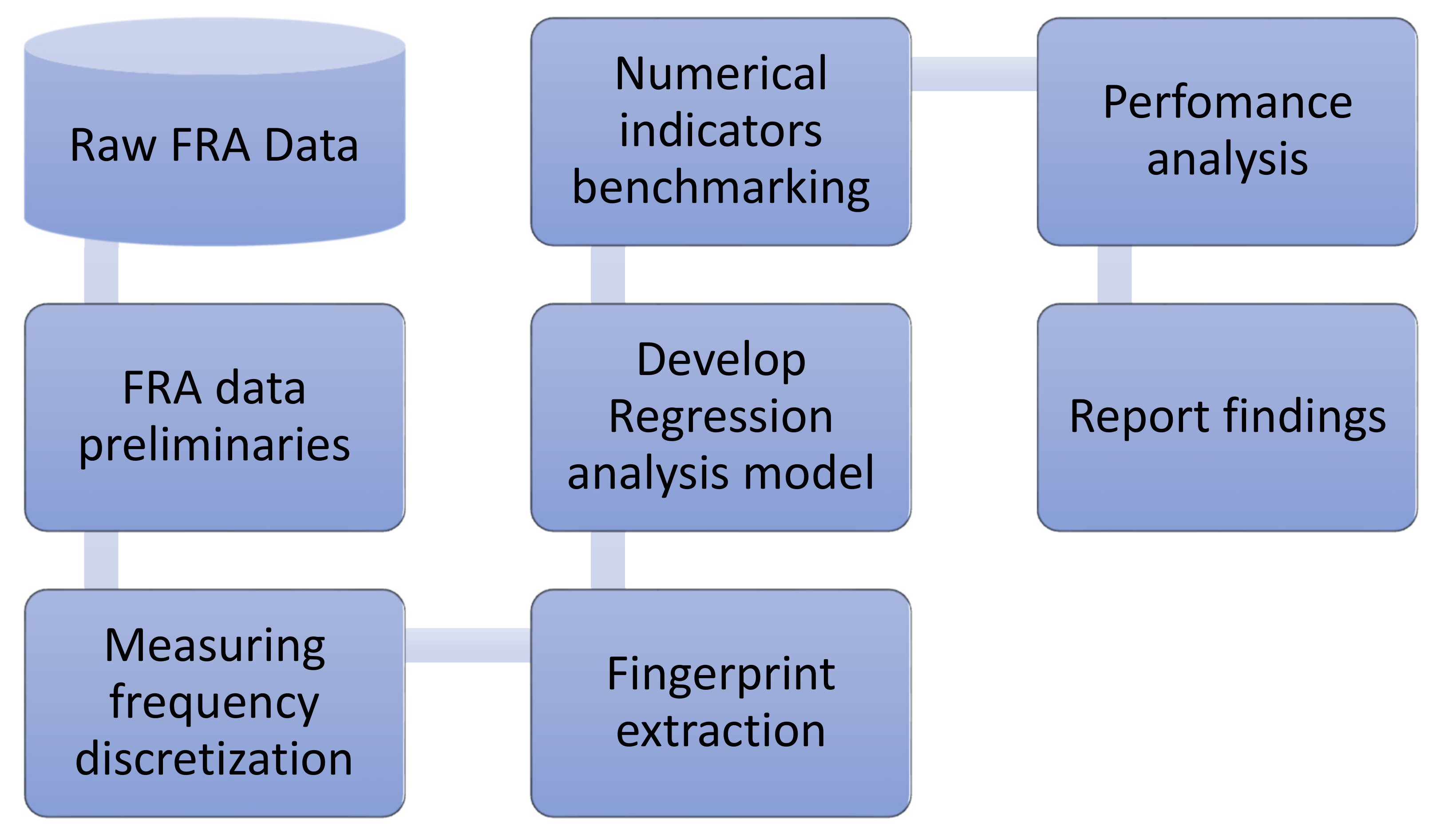
2. Materials and Methods
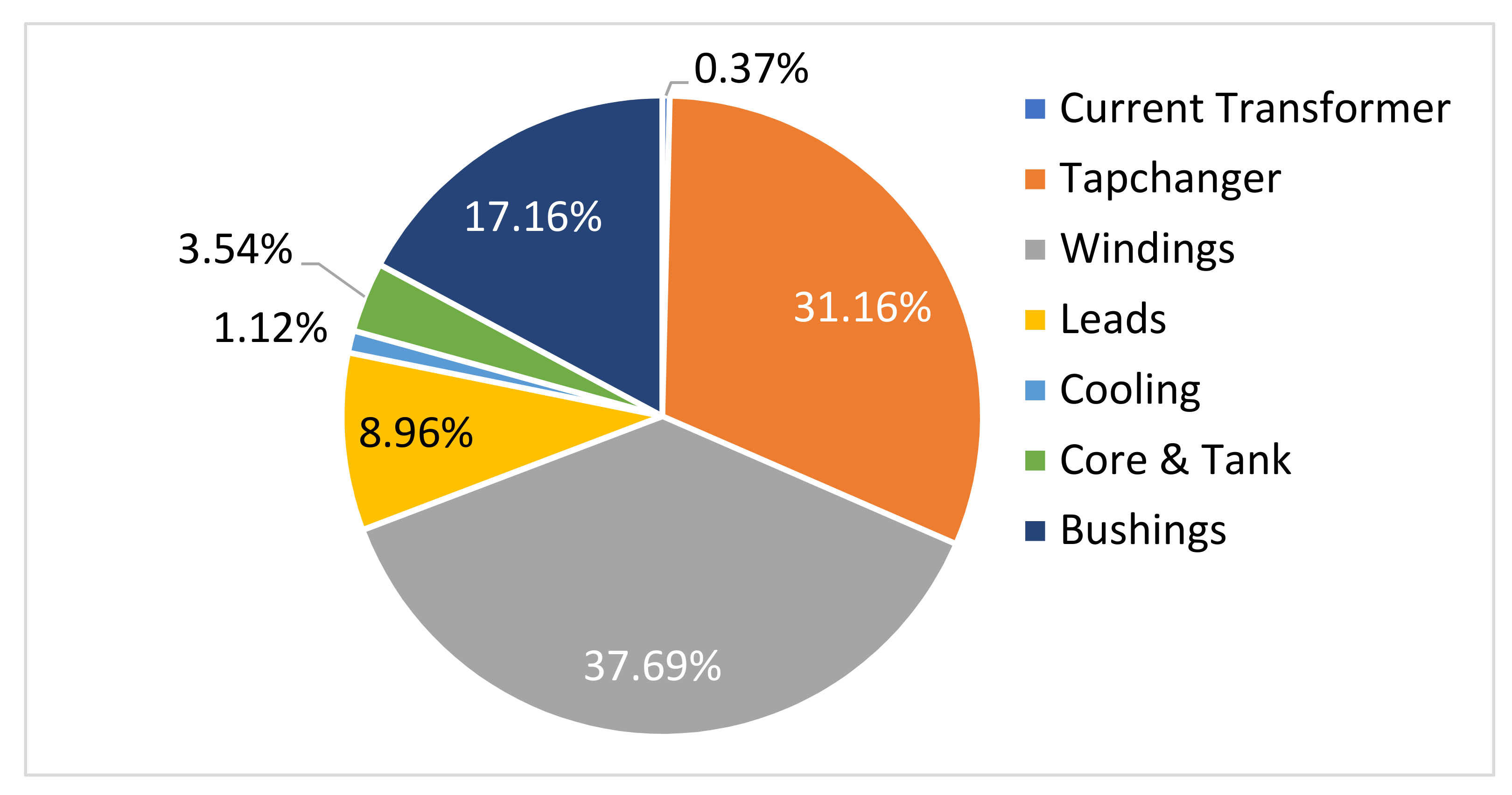
2.1. Fault Recognition Algorithm (FRA) Database
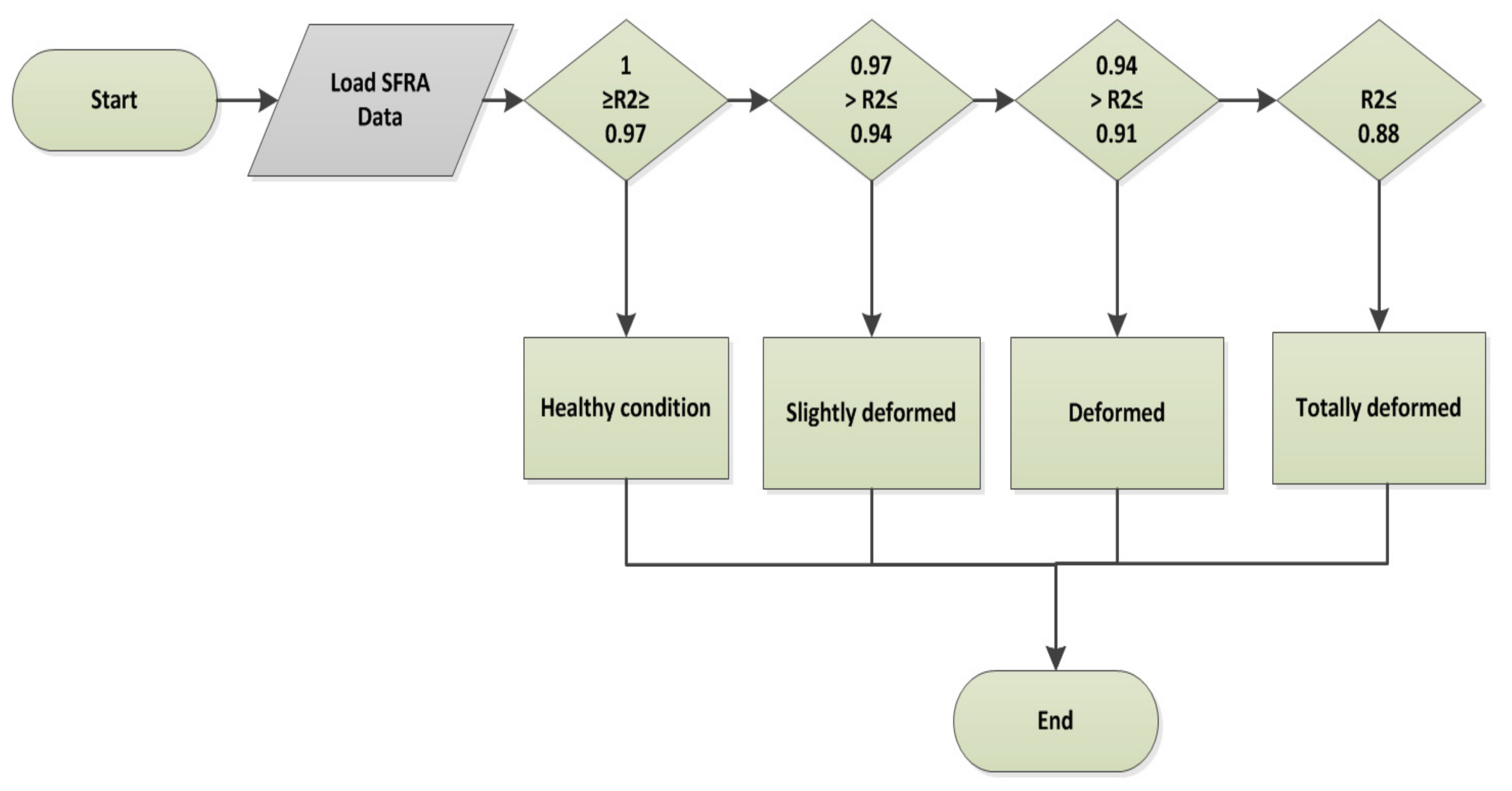
2.2. Fault Recognition Algorithm (FRA) Data Preliminaries
2.3. Fault Recognition Algorithm (FRA) Measuring Frequency Discretisation
- The FRA data of investigated transformers with known faults were compared with previous FRA data of the same unit.
- In the case where the fingerprint of the same unit was not available, the latest FRA data was compared with the same MVA unit designed according to the same technical specification.
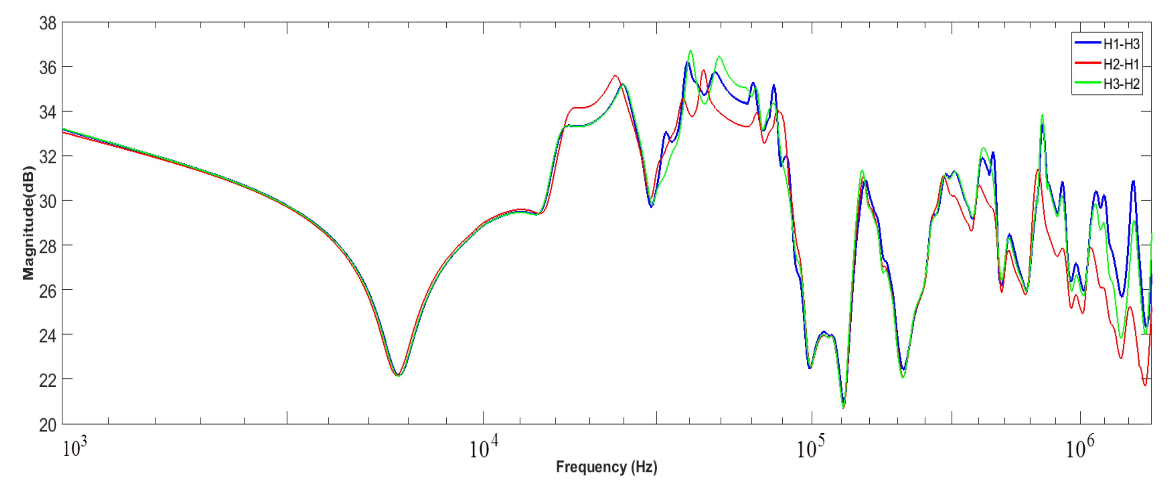
- The FRA data of one phase were compared with those of another phase of the same unit.
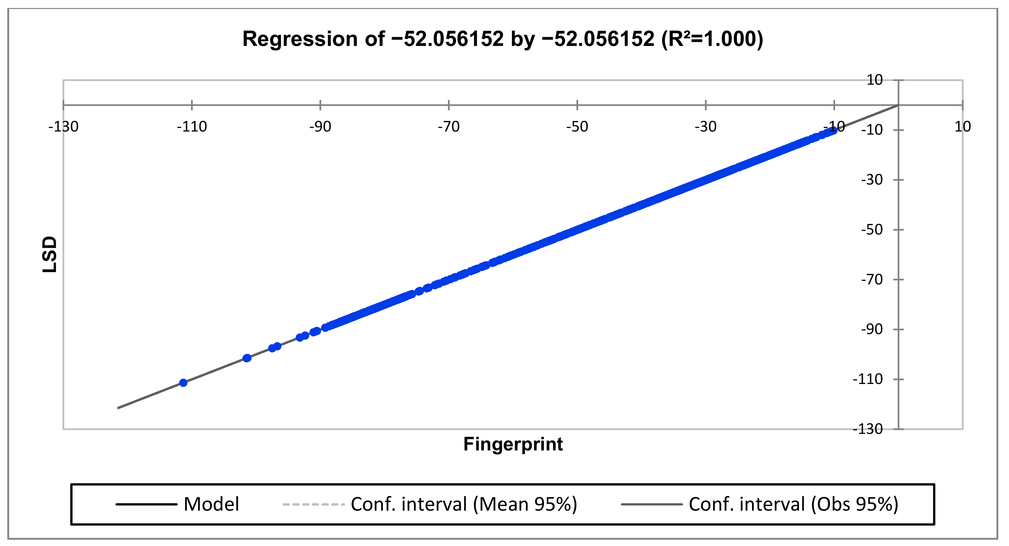
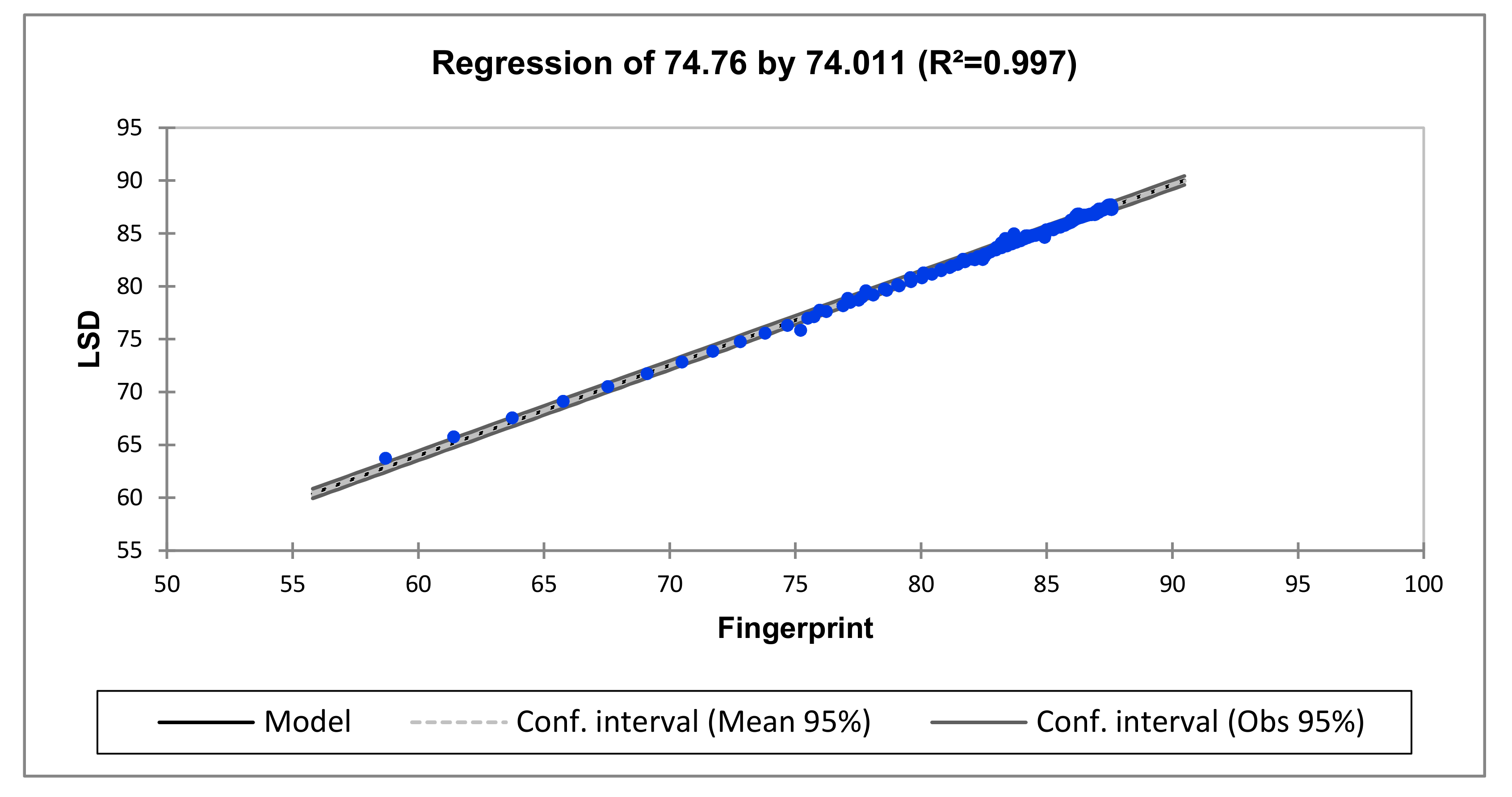
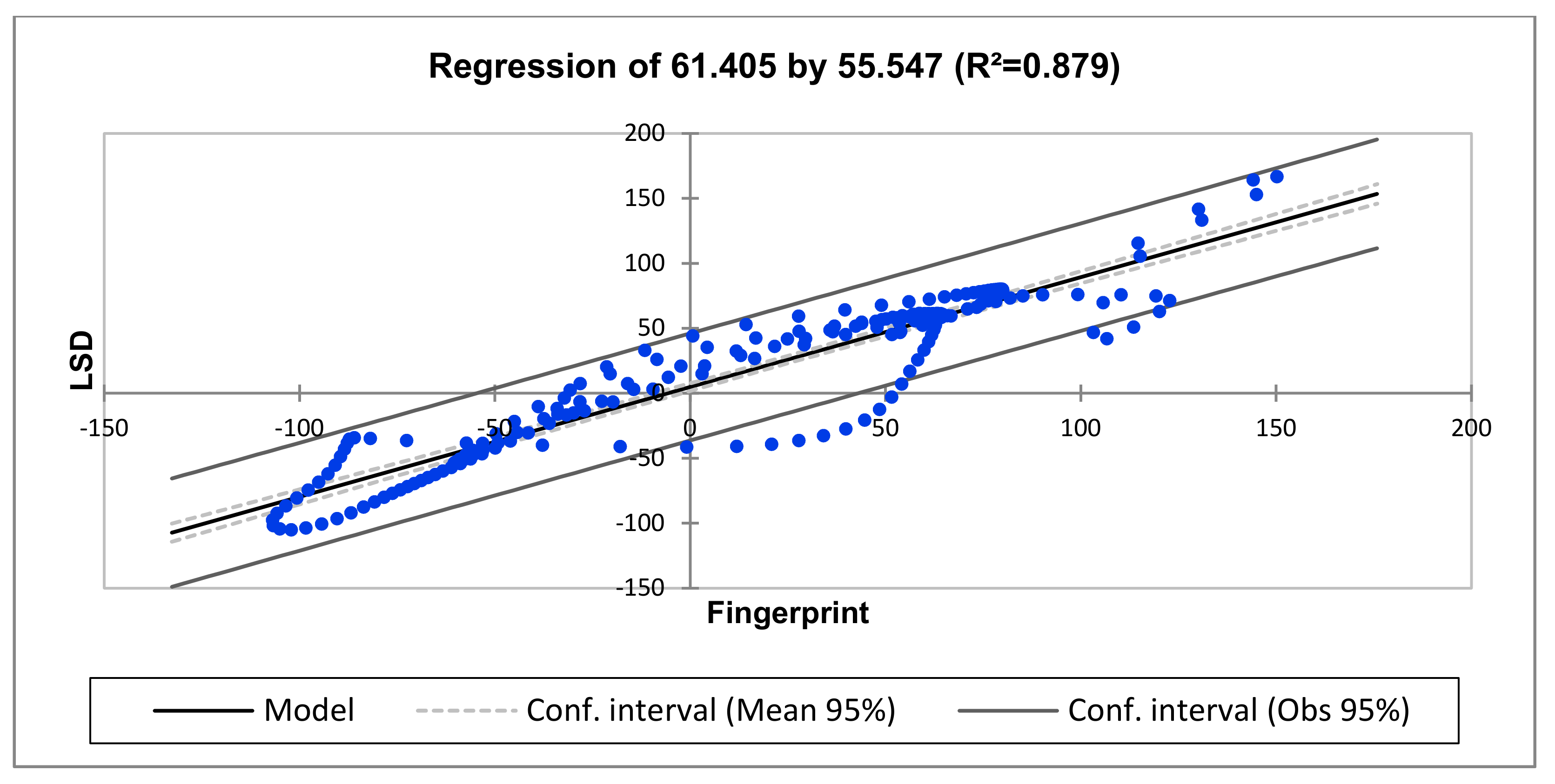
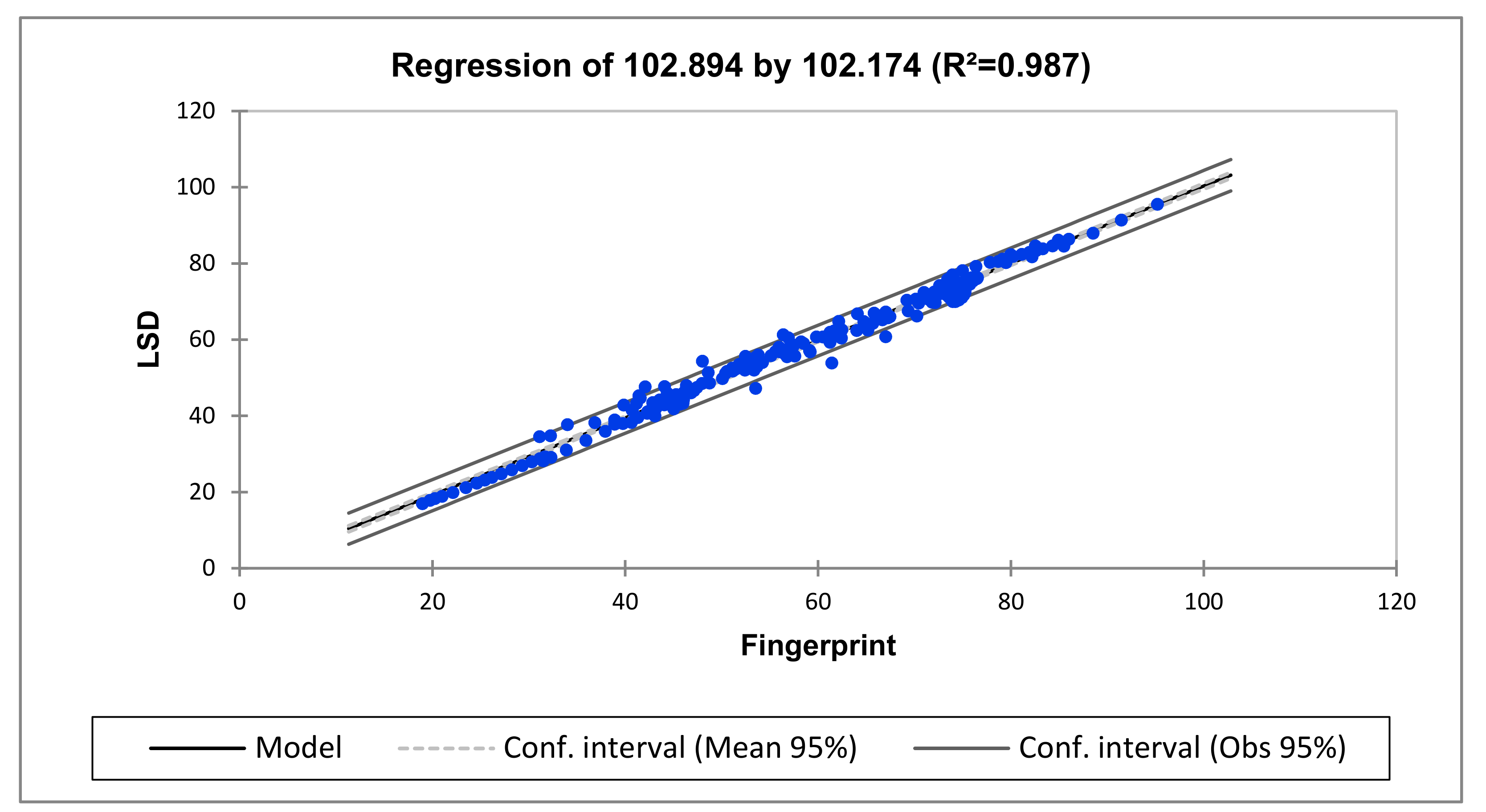
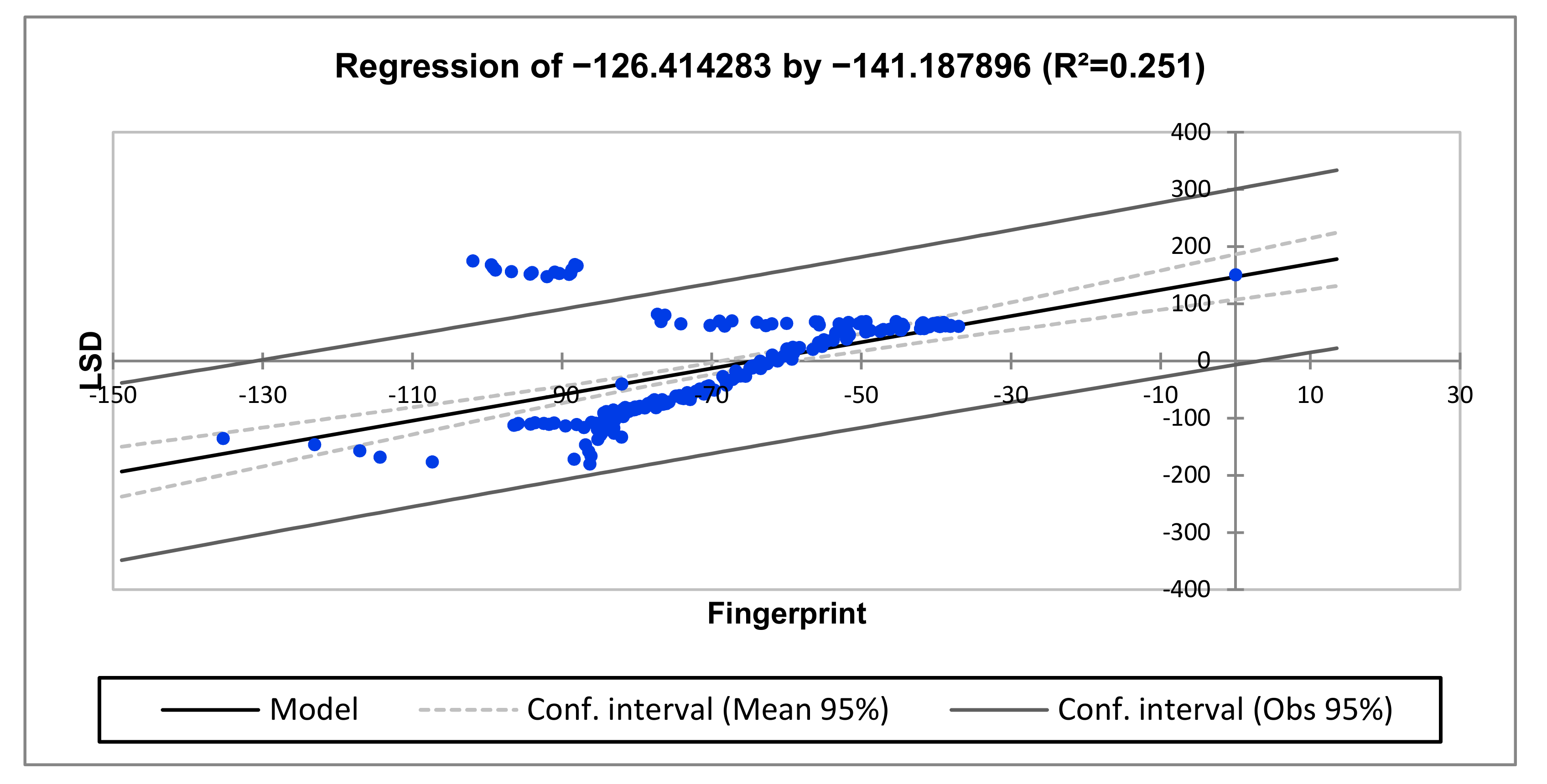
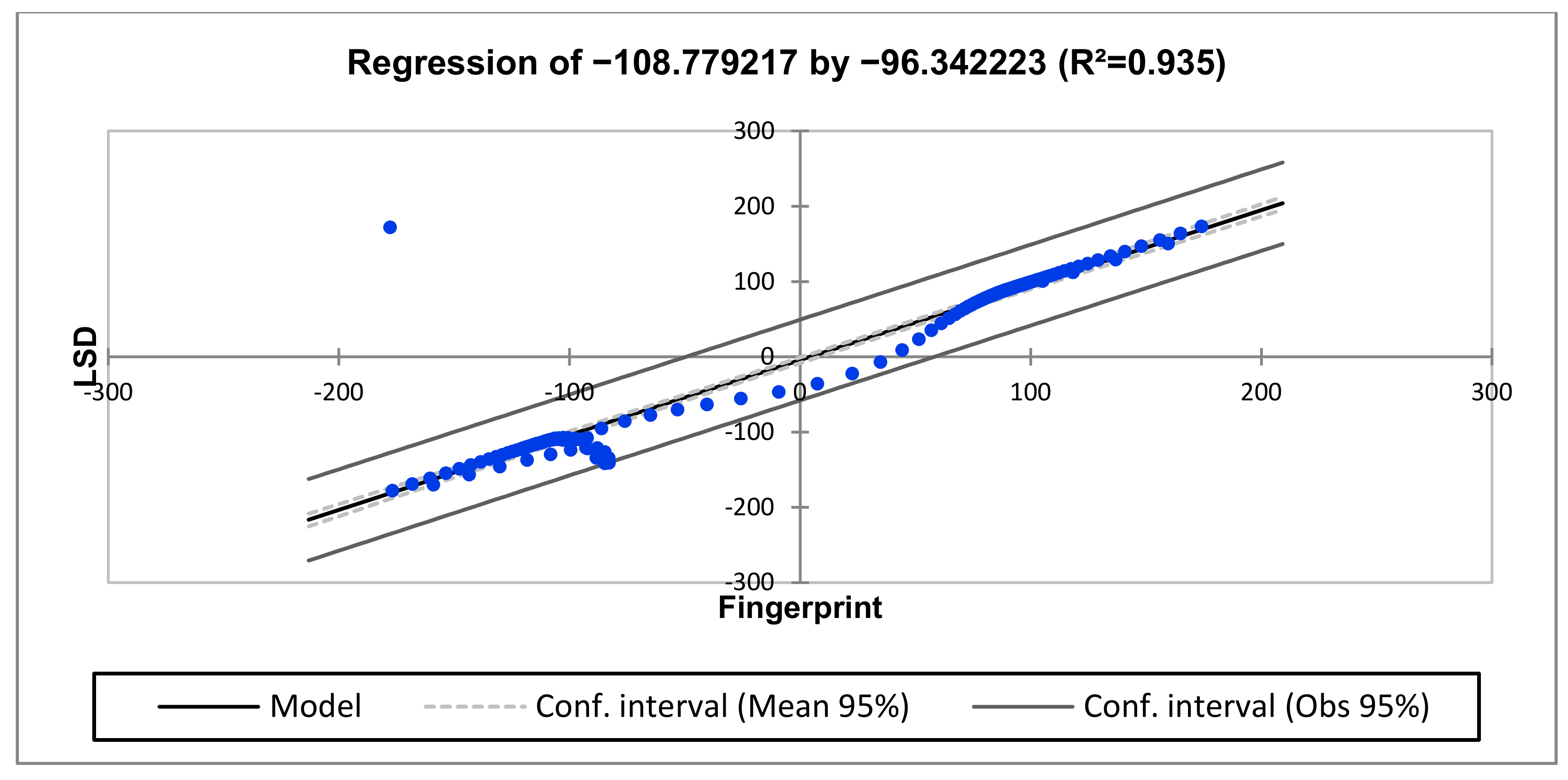
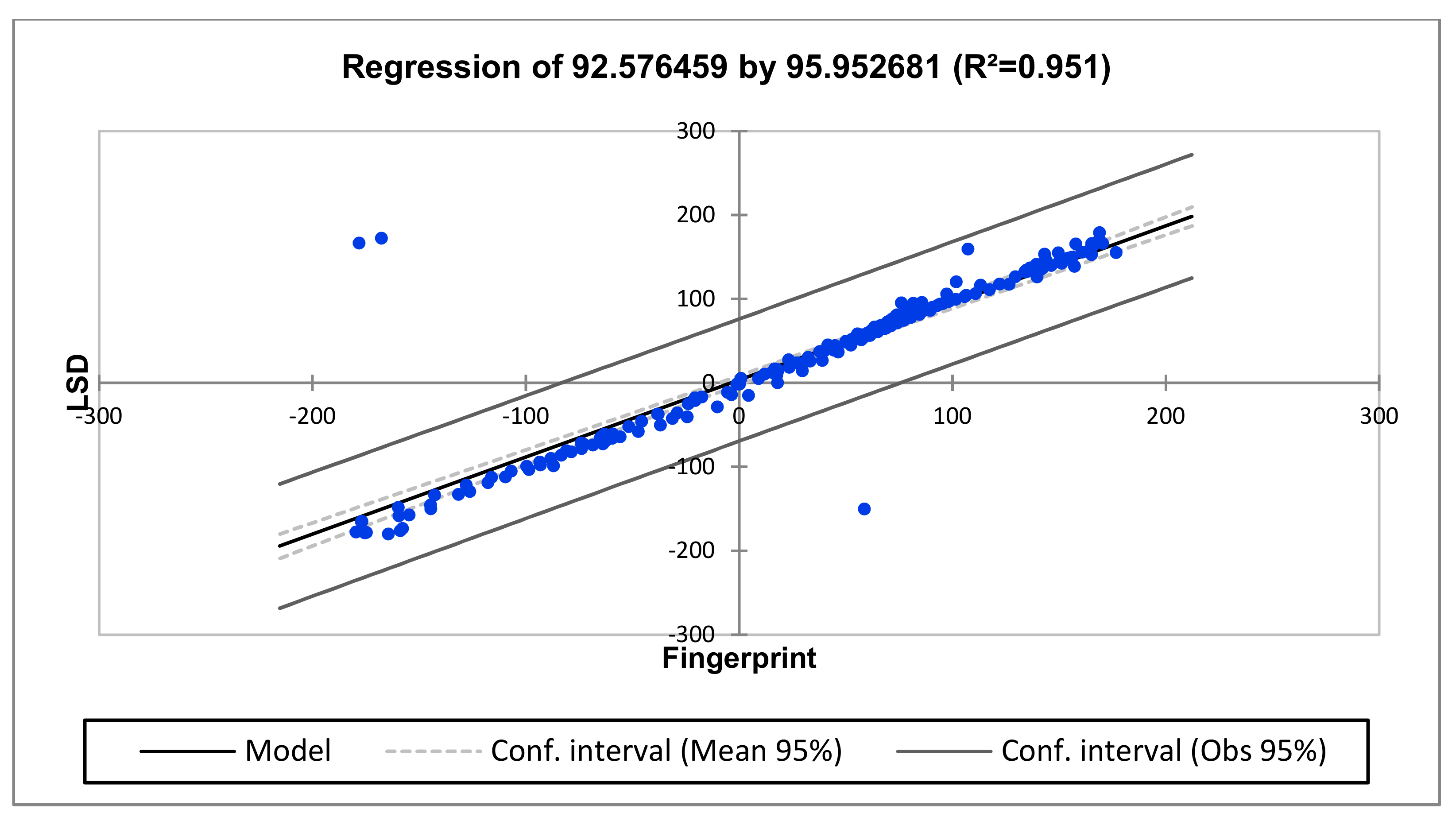
2.4. Development of Regression Analysis Model
2.5. Numerical Indicators Benchmarking
2.6. Performance Analysis
3. Results
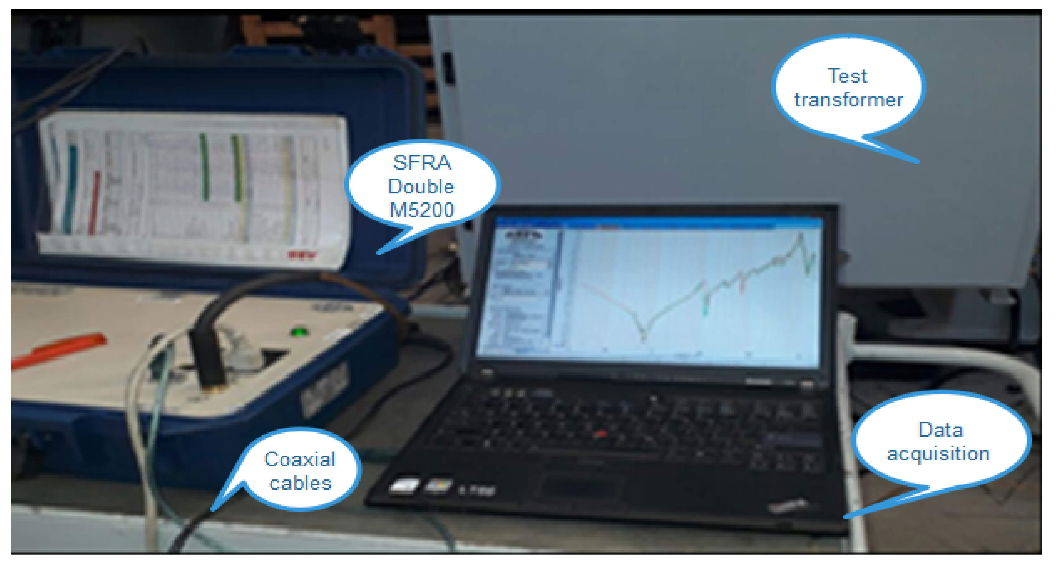
3.1. Measurement Setup
3.2. Case Studies
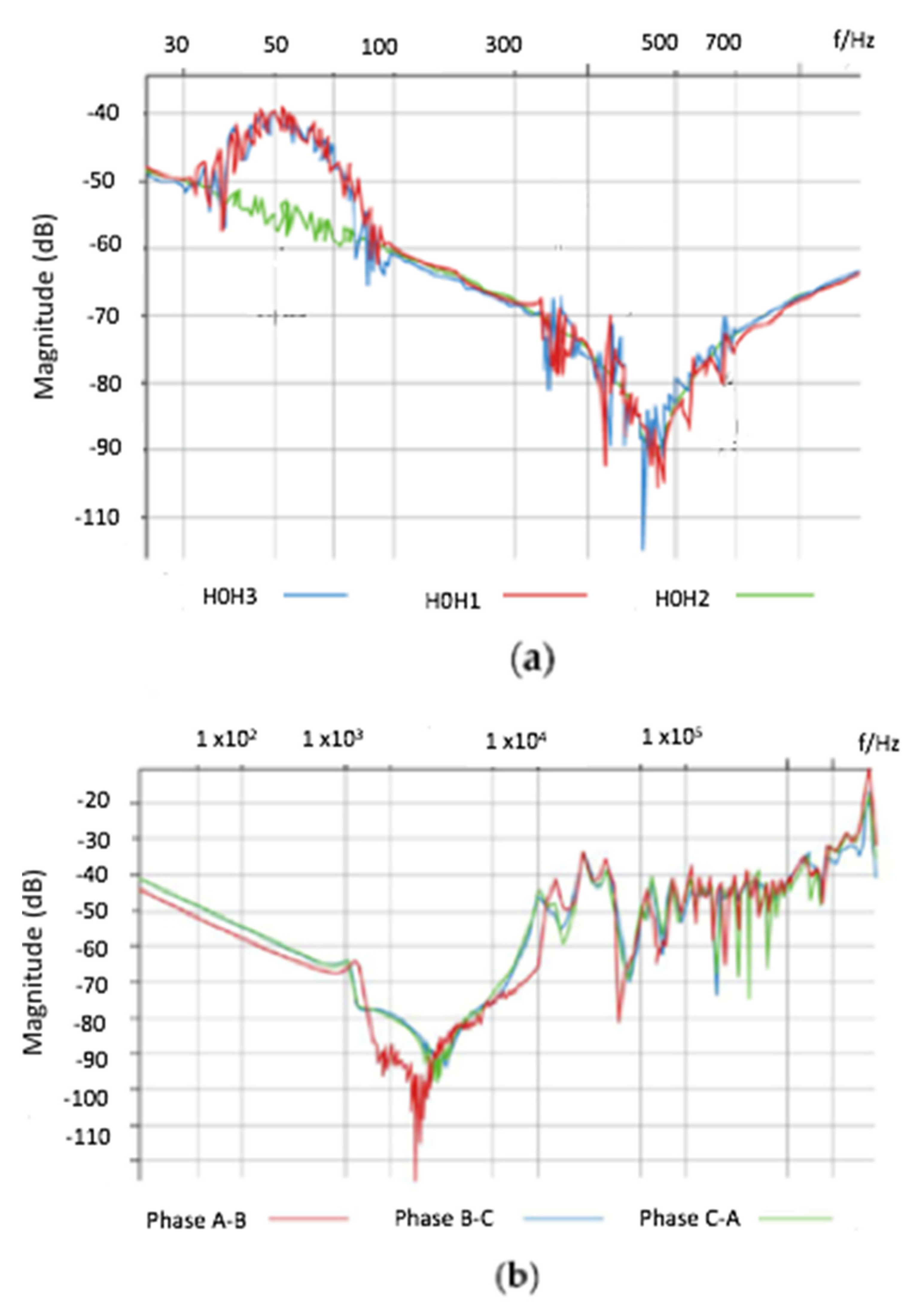
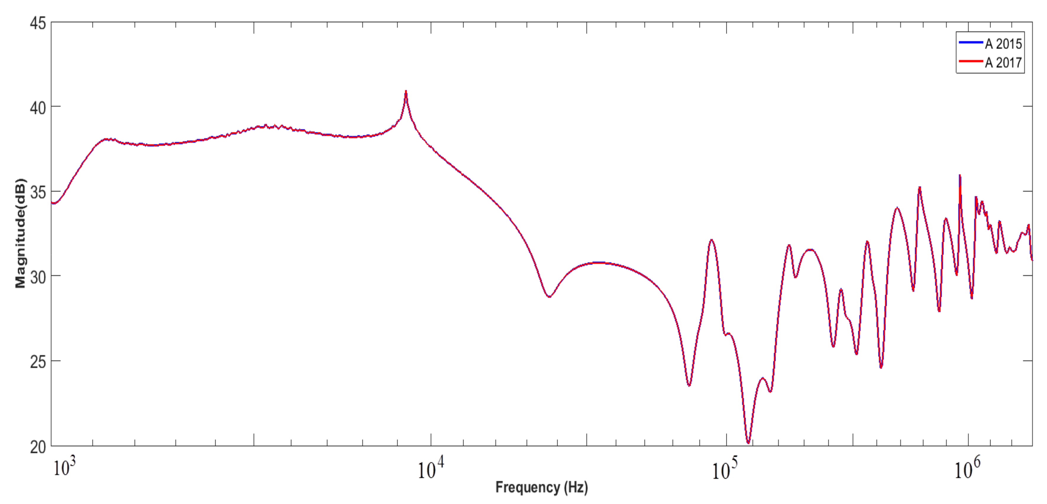
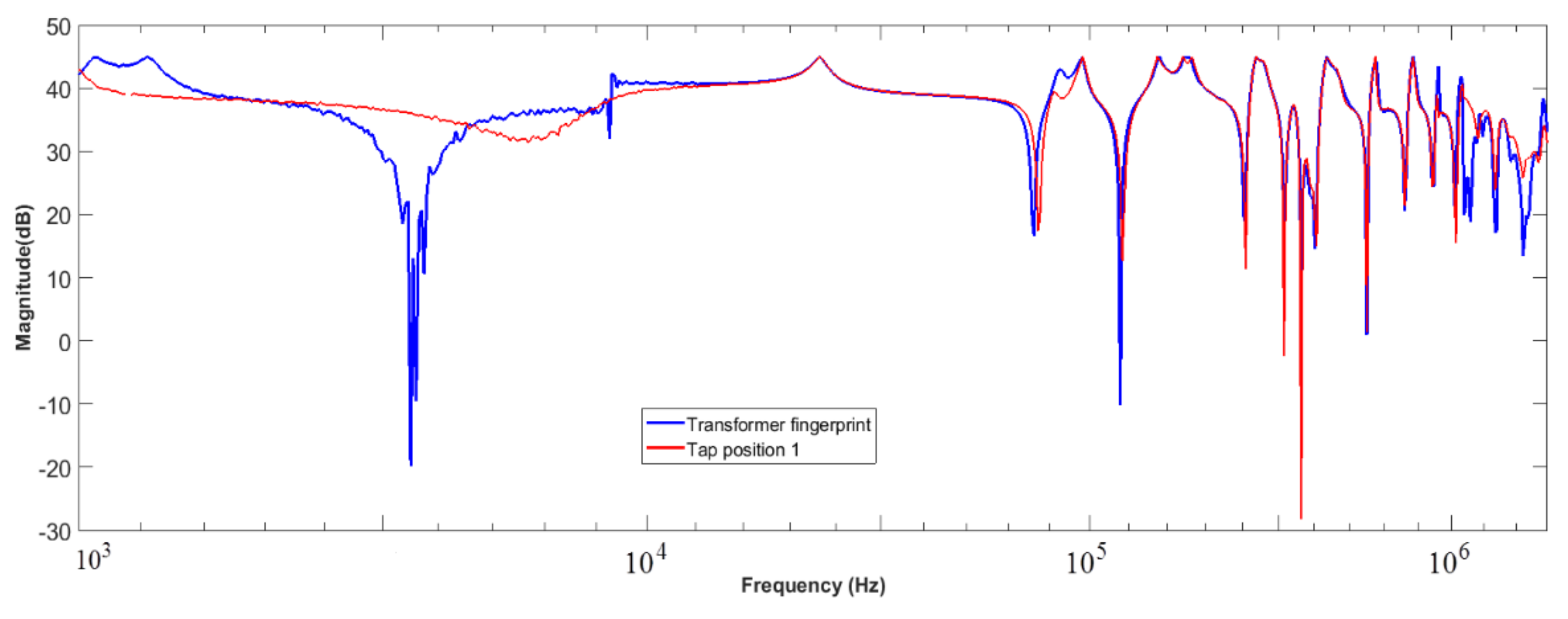
3.2.1. Investigating Frequency Response of Transformers in Good Condition
Case Study 1
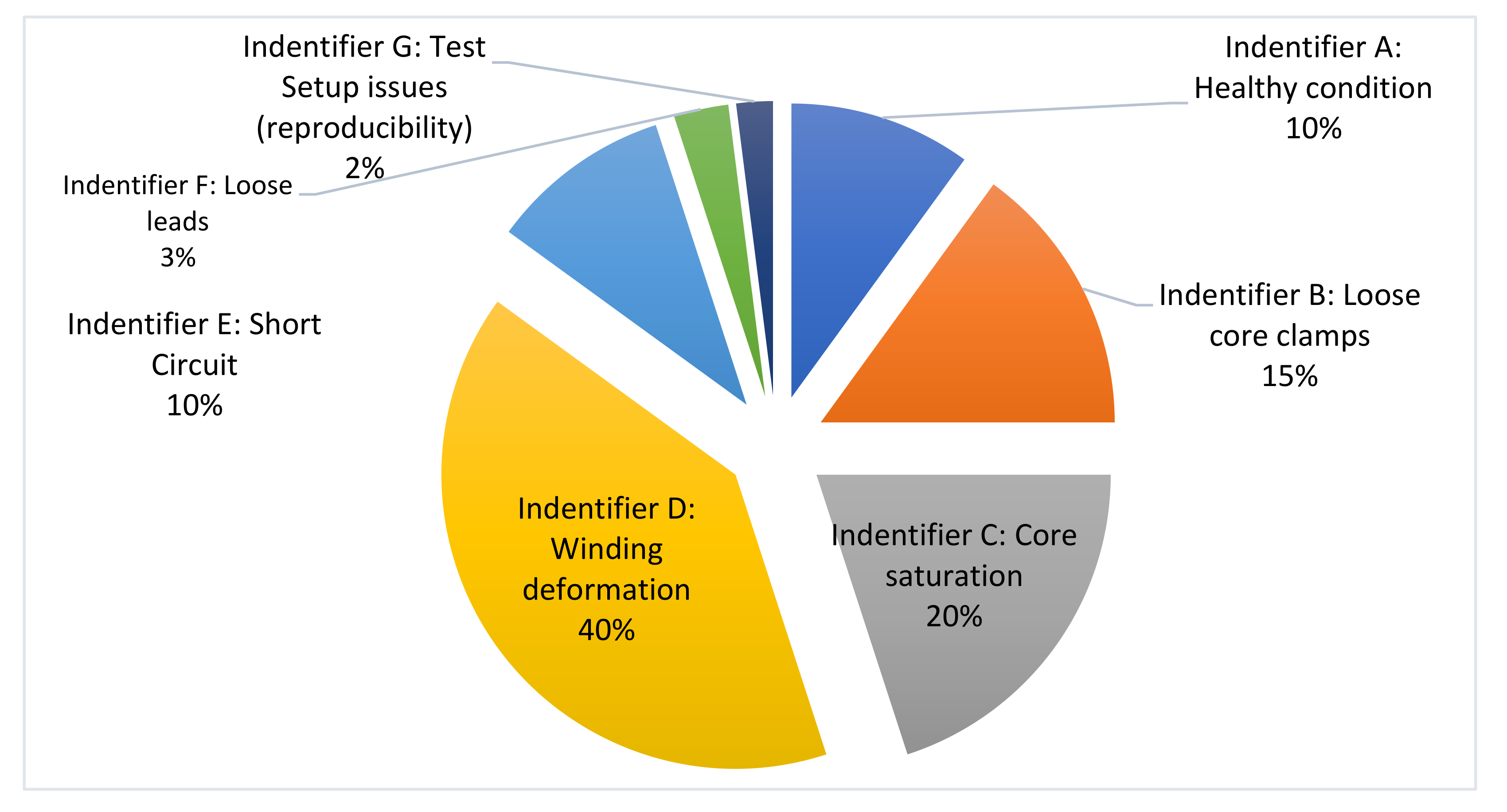
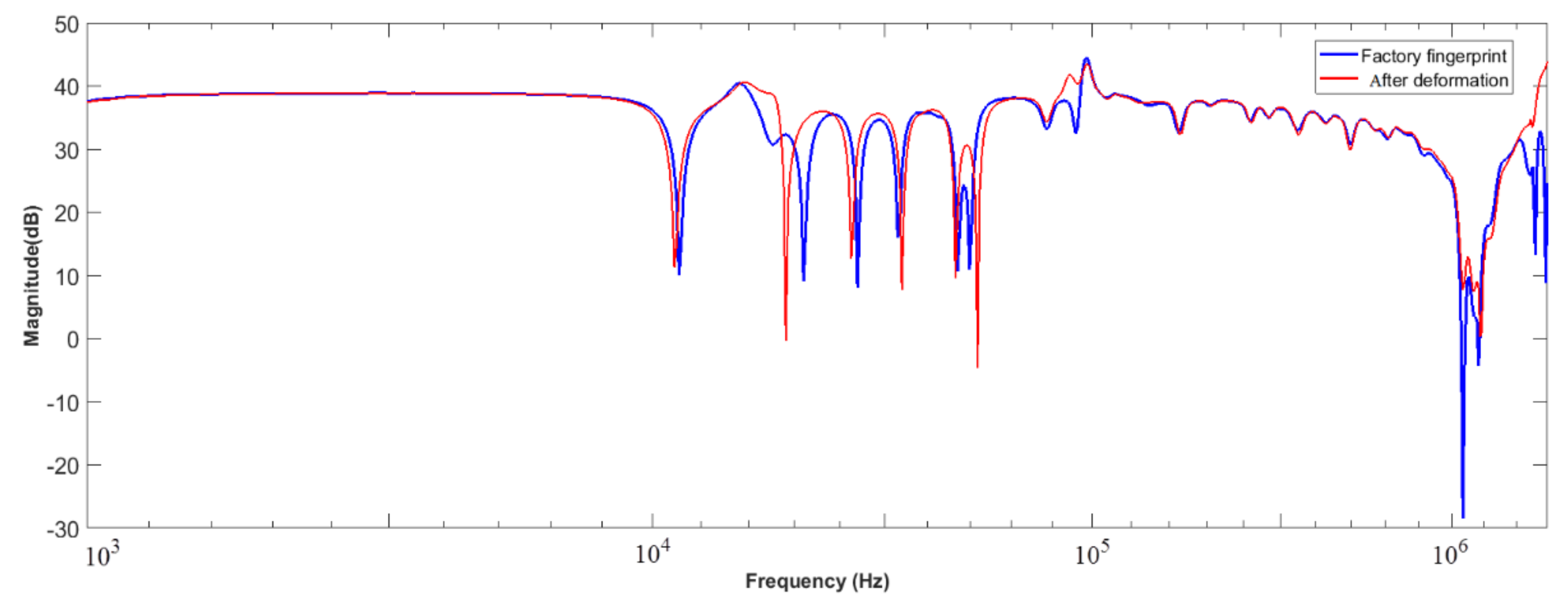
3.2.2. Investigating Frequency Response for Transformers with Winding Damages
Case Study 2
Case Study 3
Case Study 4
4. Conclusions
Author Contributions
Funding
Institutional Review Board Statement
Informed Consent Statement
Data Availability Statement
Acknowledgments
Conflicts of Interest
References
- Ramesh, K.; Sushama, M. Inter-Turn Fault Detection in Power Transformer Using Fuzzy Logic. In Proceedings of the 2014 International Conference on Science Engineering and Management Research (ICSEMR), Chennai, India, 27–29 November 2014. [Google Scholar]
- Gouda, O.E.; El Dein, A.Z.; Moukhtar, I. Turn-to-earth fault modelling of power transformer based on symmetrical components. IET Gener. Transm. Distrib. 2013, 7, 709–716. [Google Scholar] [CrossRef]
- Afkar, H.; Vahedi, A. Detecting and locating tum to tum Fault on layer winding of distribution transformer. In Proceedings of the 5th IEEE Conference on Thermal Power Plants (lPGC2014), Shahid Beheshti University, Tehran, Iran, 10–11 June 2014; pp. 109–116. [Google Scholar]
- Patel, B.; Wang, Z.; Milanovic, J.; Jarman, P. Assessing transformer reliability using post-mortem data and health indices. In Proceedings of the 2014 International Conference on Condition Monitoring and Diagnosis (CMD), Jesu, Korea, 21–25 September 2014; pp. 472–475. [Google Scholar]
- Behjat, V. Diagnosing Shorted Turns on the Windings of Power Transformers Based Upon Online FRA Using Capacitive and Inductive Couplings. IEEE Trans. Power Deliv. 2011, 26, 2123–2133. [Google Scholar] [CrossRef]
- Tenbohlen, S. Transformer Reliability Survey; Technical Brochure 642 CIGRE; CIGRE: Paris, France, 2015. [Google Scholar]
- Tenbohlen, S.; Lapworth, M. Development and results of a worldwide transformer reliability survey. In Proceedings of the CIGRE SC A2 Colloquium, Shanghai, China, 20–25 September 2015. [Google Scholar]
- Ahn, H.M.; Lee, J.Y.; Kim, J.K.; Oh, Y.H.; Jung, S.Y.; Hahn, S.C. Finite-Element Analysis of Short-Circuit Electromagnetic Force in Power Transformer. IEEE Trans. Ind. Appl. 2011, 47, 1267–1272. [Google Scholar]
- Abu-Siada, A.; Hashemnia, N.; Islam, S.; Masoum, M.A. Understanding power transformer frequency response analysis signatures. IEEE Electr. Insul. Mag. 2013, 29, 48–56. [Google Scholar] [CrossRef]
- Dick, E.P.; Erven, C.C. Transformer Diagnostic Testing by Frequency Response Analysis. IEEE Trans. Power Appar. Syst. 1978, 6, 2144–2153. [Google Scholar] [CrossRef]
- Nyandeni, D.B.; Phoshoko, M.; Murray, R.; Thango, B.A. Transformer Oil Degradation on PV Plants—A Case Study. In Proceedings of the 8th South African Regional Conference (CIGRE), Johannesburg, South Africa, 14–17 November 2017. [Google Scholar]
- IEEE. IEEE Recommended Practice for Validation of Computational Electromagnetics Computer Modeling and Simulations. 2011. Available online: http://ieeexplore.ieee.org/document/5721917/ (accessed on 15 January 2022).
- Tahir, M.; Tenbohlen, S. Transformer Winding Condition Assessment Using Feedforward Artificial Neural Network and Frequency Response Measurements. Energies 2021, 14, 3227. [Google Scholar] [CrossRef]
- Zambrano, G.M.V.; Ferreira, A.C.; Caloba, L.P. Power transformer equivalent circuit identification by artificial neural network using frequency response analysis. In Proceedings of the 2006 IEEE Power Engineering Society General Meeting, Montreal, QC, Canada, 18–22 June 2006; p. 6. [Google Scholar] [CrossRef]
- Singh, J.; Sood, Y.R.; Jarial, R.K. Novel method for detection of transformer winding faults using Sweep Frequency Response Analysis. In Proceedings of the Power Engineering Society General Meeting, Tampa, FL, USA, 24–28 June 2007. [Google Scholar]
- Sathya, M.A. Prediction of Transformer Winding Displacement from Frequency Response Characteristics. In Proceedings of the 2013 IEEE 1st International Conference on Condition Assessment Techniques in Electrical Systems, Kolkata, India, 6–8 December 2013. [Google Scholar]
- Waters, M. The Short-Circuit Strength of Power Transformers; McDonald & Co., Ltd.: London, UK, 1966. [Google Scholar]
- Miroslav, G. Experimental Analysis of Short-Circuit Effects in Transformer Winding by Impact Test and SFRA. In Proceedings of the 2016 Diagnostic of Electrical Machines and Insulating Systems in Electrical Engineering (DEMISEE), Papradno, Slovakia, 20–22 June 2016. [Google Scholar]
- Rahman, M.A.A. The Effects of Short-Circuit and Inrush Currents on HTS Transformer Windings. IEEE Trans. Appl. Supercond. 2012, 22, 5500108. [Google Scholar] [CrossRef]
- Kulkarni, S.V.; Khaparde, S.A. Transformer Engineering Design and Practice; Marcel Dekker: New York, NY, USA, 2004. [Google Scholar]
- Abdi, S.; Harid, N.; Safiddine, L.; Boubakeur, A.; Haddad, A. The Correlation of Transformer Oil Electrical Properties with Water Content Using a Regression Approach. Energies 2021, 14, 2089. [Google Scholar] [CrossRef]
- Tamus, Z.Á. Regression analysis to evaluate the reliability of insulation diagnostic methods. J. Electrost. 2013, 3, 564–567. [Google Scholar] [CrossRef]
- Gopalakrishna, S.; Kumar, K.; George, B.; Jayashankar, V. Design margin for short circuit withstand capability in large power transformer. In Proceedings of the 8th International Power Engineering, Singapore, 3–6 December 2007. [Google Scholar]
- Ghani, S.A.; Thayoob, Y.M.; Ghazali, Y.; Khiar, M. Evaluation of transformer core and winding conditions from SFRA measurement results using statistical techniques for distribution transformers. In Proceedings of the 2012 IEEE International Power Engineering and Optimization Conference, Melaka, Malaysia, 6–7 June 2012; pp. 448–453. [Google Scholar]
- Banaszak, S.; Szoka, W. Transformer Frequency Response Analysis With the Grouped Indices Method in End-to-End and Capacitive Inter-Winding Measurement Configurations. IEEE Trans. Power Deliv. 2020, 35, 571–579. [Google Scholar] [CrossRef]


| Frequency Region | Transformer Component | Influencing Elements |
|---|---|---|
| 1–10 kHz | Main core Winding inductance | Core deformation, open circuits, shorted turns and residual magnetism |
| 10–100 kHz | Bulk component Main windings | Deformation within the main or tap windings Bulk winding movement between windings and clamping structure |
| 400 kHz–1 MHz | Main windings Tap windings Internal leads | Movement of the main and tap windings, ground impedance variations |
| Case # | Location | Power Rating | Voltage Ratings |
|---|---|---|---|
| 1 | Gauteng | 20 MVA | 132/11 kV |
| 2 | Gauteng | 50 MVA | 66/11.66 kV |
| 3 | North West | 40 MVA | 132/11 kV |
| 4 | North West | 10 MVA | 66/11 kV |
| Technique | Frequency Region | ||
|---|---|---|---|
| Low (1–10 kHz) | Medium (10–100 kHz) | High (100 kHz–1 MHz) | |
| CC | 1 | 1 | 1 |
| ASLE | 0 | 0 | 0 |
| The Goodness of Fit Statistics | Frequency Region | ||
|---|---|---|---|
| Low (1–10 kHz) | Medium (10–100 kHz) | High (100 kHz–1 MHz) | |
| Std. deviation | 0 | 0 | 0 |
| R2 | 1 | 1 | 1 |
| Adjusted R2 | 1 | 1 | 1 |
| Technique | Frequency Region | ||
|---|---|---|---|
| Low (1–10 kHz) | Medium (10–100 kHz) | High (100 kHz–1 MHz) | |
| CC | 0.998 | 0.8909 | 0.9981 |
| ASLE | 0.02 | 0.3330 | 0.034 |
| The Goodness of Fit Statistics | Frequency Region | ||
|---|---|---|---|
| Low (1–10 kHz) | Medium (10–100 kHz) | High (100 kHz–1 MHz) | |
| Std. deviation | 4.242 | 19.789 | 17.615 |
| R2 | 0.997 | 0.879 | 0.987 |
| Adjusted R2 | 0.997 | 0.878 | 0.987 |
| Technique | Frequency Region | ||
|---|---|---|---|
| Low (1–10 kHz) | Medium (10–100 kHz) | High (100 kHz–1 MHz) | |
| CC | 0.5057 | 0.9121 | 0.9798 |
| ASLE | 1 | 0.1734 | 0.0475 |
| The Goodness of Fit Statistics | Frequency Region | ||
|---|---|---|---|
| Low (1–10 kHz) | Medium (10–100 kHz) | High (100 kHz–1 MHz) | |
| Std. deviation | 26.858 | 3.12 | 1.351 |
| R2 | 0.251 | 0.935 | 0.951 |
| Adjusted R2 | 0.248 | 0.935 | 0.838 |
| Frequency Region | Equation of the Model |
|---|---|
| Low (1–10 kHz) | LSD = 147.0374 + 2.2869 × Fingerprint |
| Medium (10–100 kHz) | LSD = −4.3357 + 0.9963 × Fingerprint |
| High (100 kHz–1 MHz) | LSD = 3.3804 + 0.9187 × Fingerprint |
| Technique | Frequency Region | ||
|---|---|---|---|
| Low (1–10 kHz) | Medium (10–100 kHz) | High (100 kHz–1 MHz) | |
| CC | 0.999 | 0.9191 | 0.0921 |
| ASLE | 0.03 | 0.9632 | 0.125 |
| Technique | Frequency Region | ||
|---|---|---|---|
| Low (1–10 kHz) | Medium (10–100 kHz) | High (100 kHz–1 MHz) | |
| CC | 0.999 | 0.8804 | 0.9316 |
| ASLE | 0.0493 | 0.346 | 0.432 |
| Technique | Frequency Region | ||
|---|---|---|---|
| Low (1–10 kHz) | Medium (10–100 kHz) | High (100 kHz–1 MHz) | |
| CC | 1.000 | 0.9597 | 0.9865 |
| ASLE | 0.0225 | 0.9823 | 0.536 |
| The Goodness of Fit Statistics | Frequency Region | ||
|---|---|---|---|
| Low (1–10 kHz) | Medium (10–100 kHz) | High (100 kHz–1 MHz) | |
| Std. deviation | 0.256 | 12.176 | 8.236 |
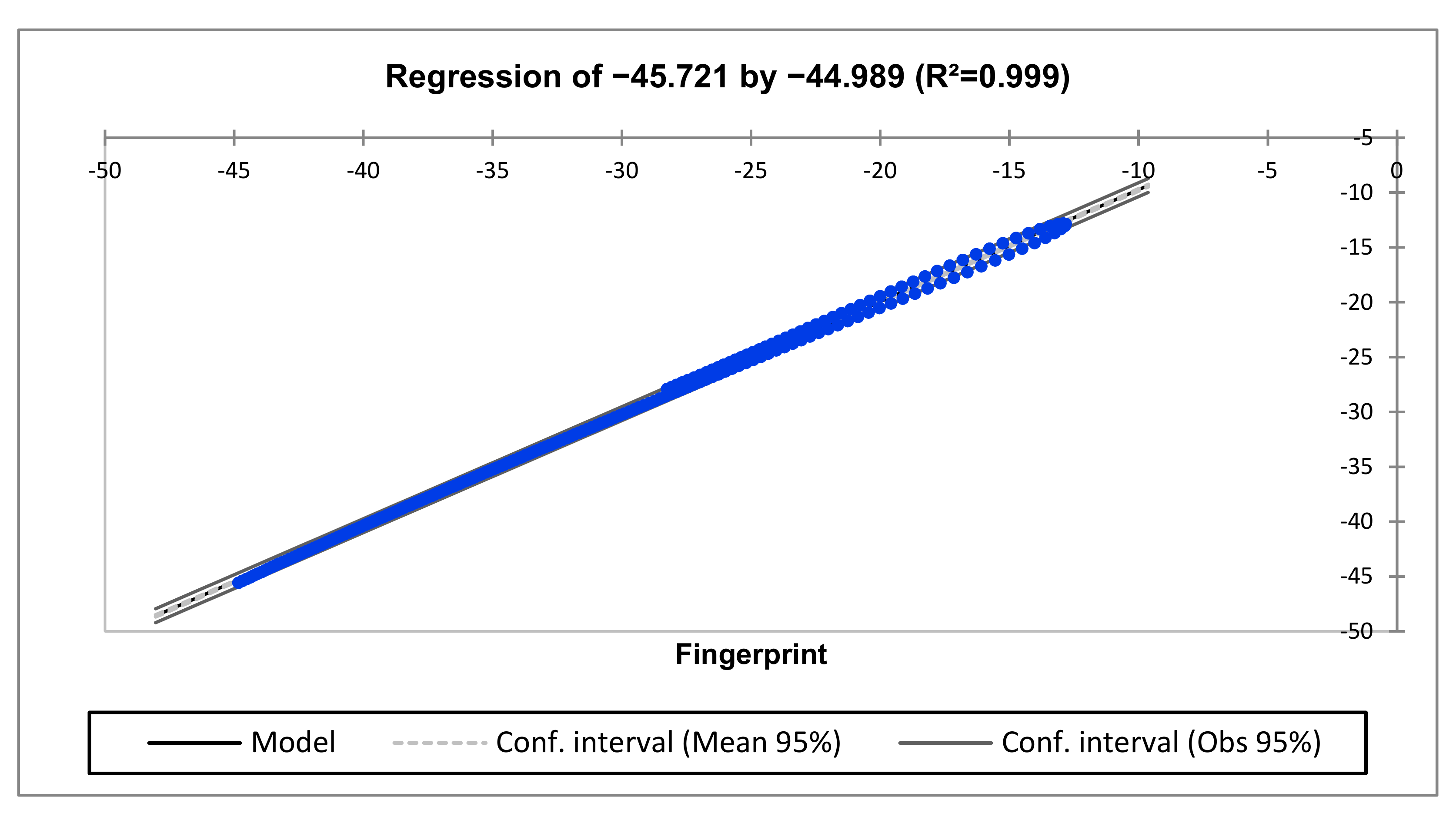
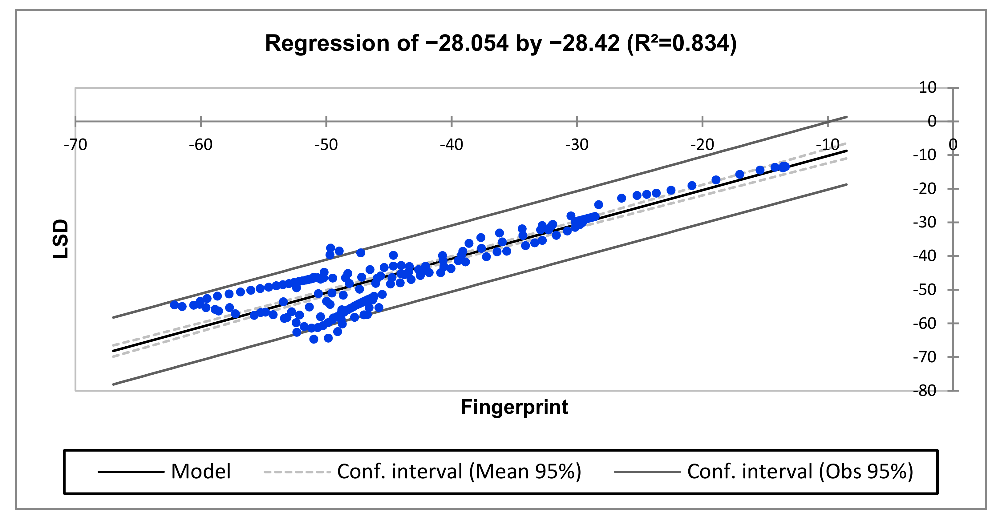
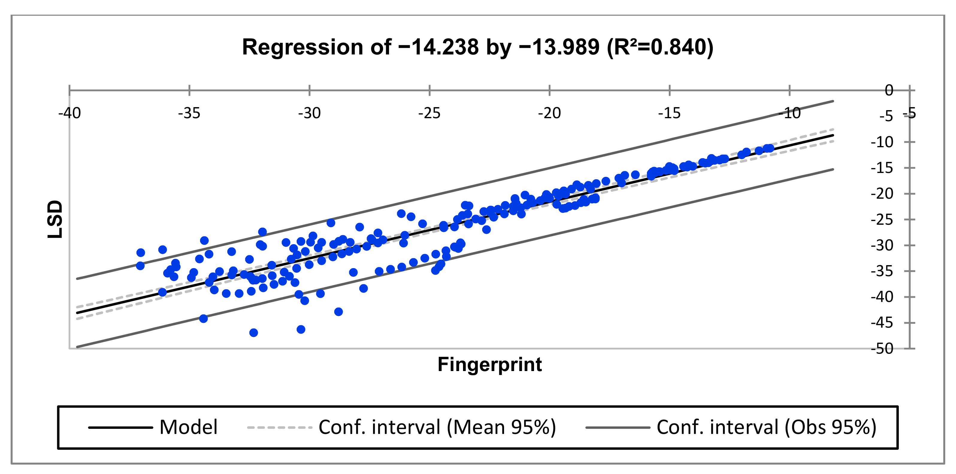
| R2 | 0.999 | 0.834 | 0.840 |
| Adjusted R2 | 0.999 | 0.833 | 0.839 |
| The Goodness of Fit Statistics | Frequency Region | ||
|---|---|---|---|
| Low (1–10 kHz) | Medium (10–100 kHz) | High (100 kHz–1 MHz) | |
| Std. deviation | 0.064 | 10.935 | 6.907 |
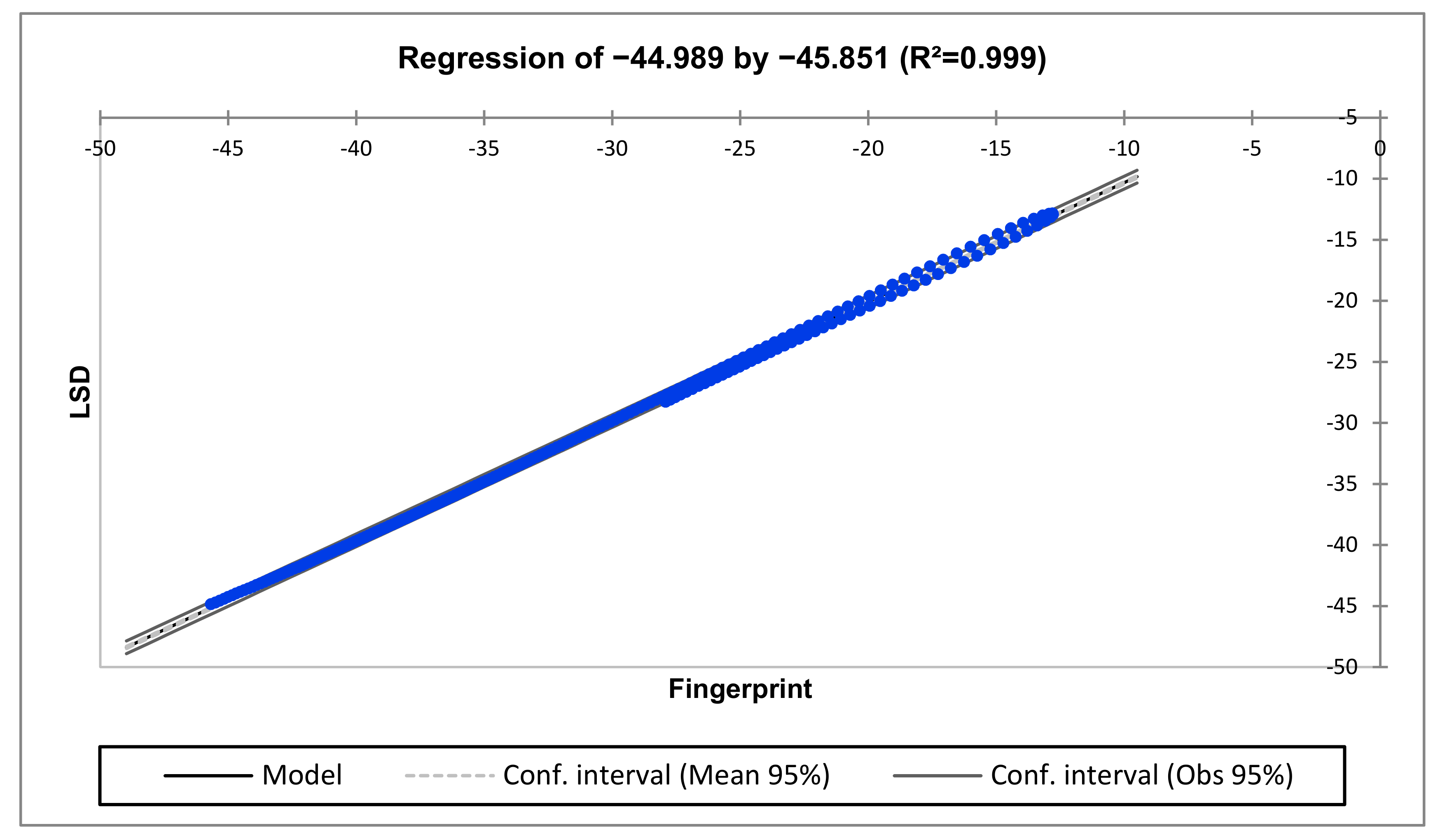
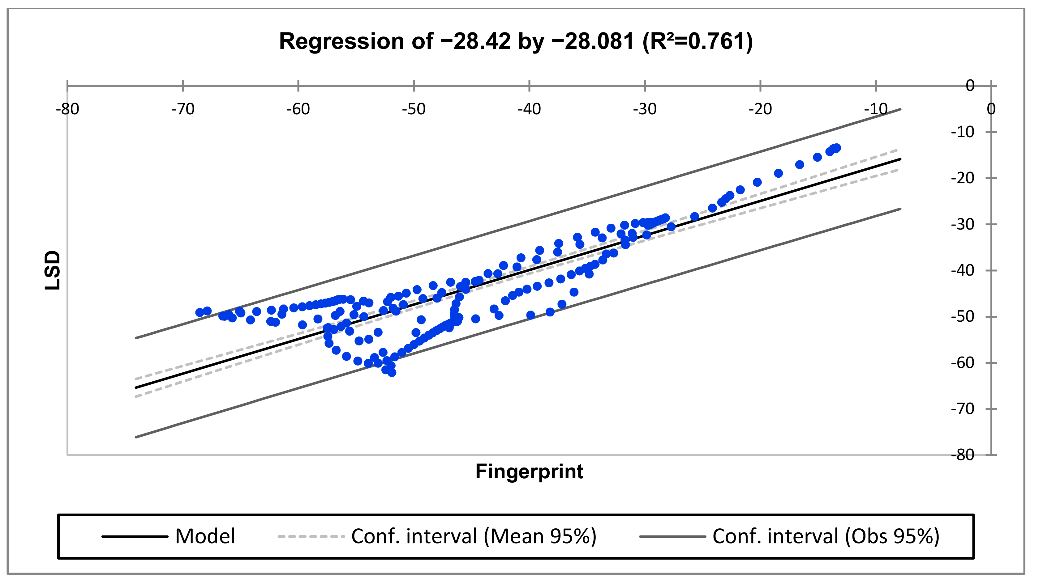
| R2 | 0.999 | 0.761 | 0.861 |
| Adjusted R2 | 0.999 | 0.760 | 0.860 |
| The Goodness of Fit Statistics | Frequency Region | ||
|---|---|---|---|
| Low (1–10 kHz) | Medium (10–100 kHz) | High (100 kHz–1 MHz) | |
| Std. deviation | 0.280 | 12.744 | 8.457 |
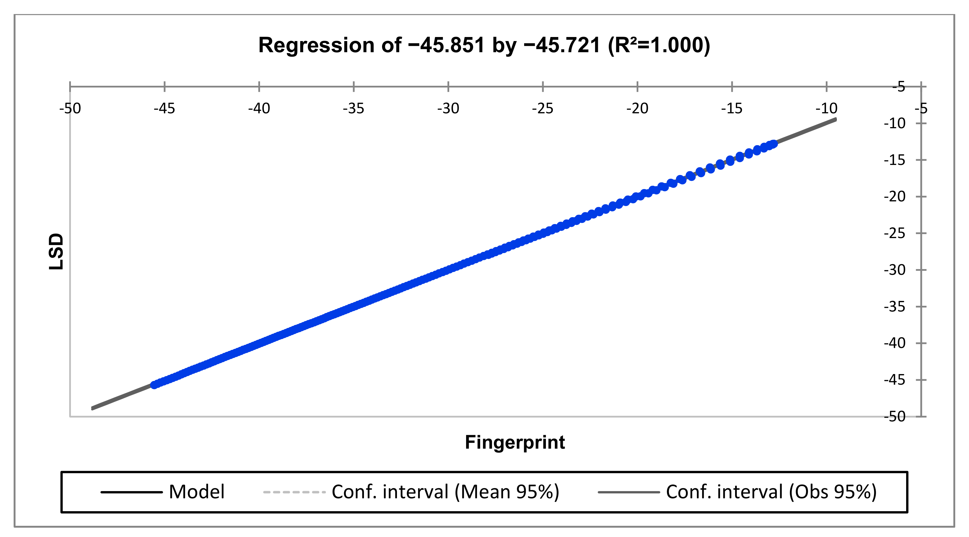
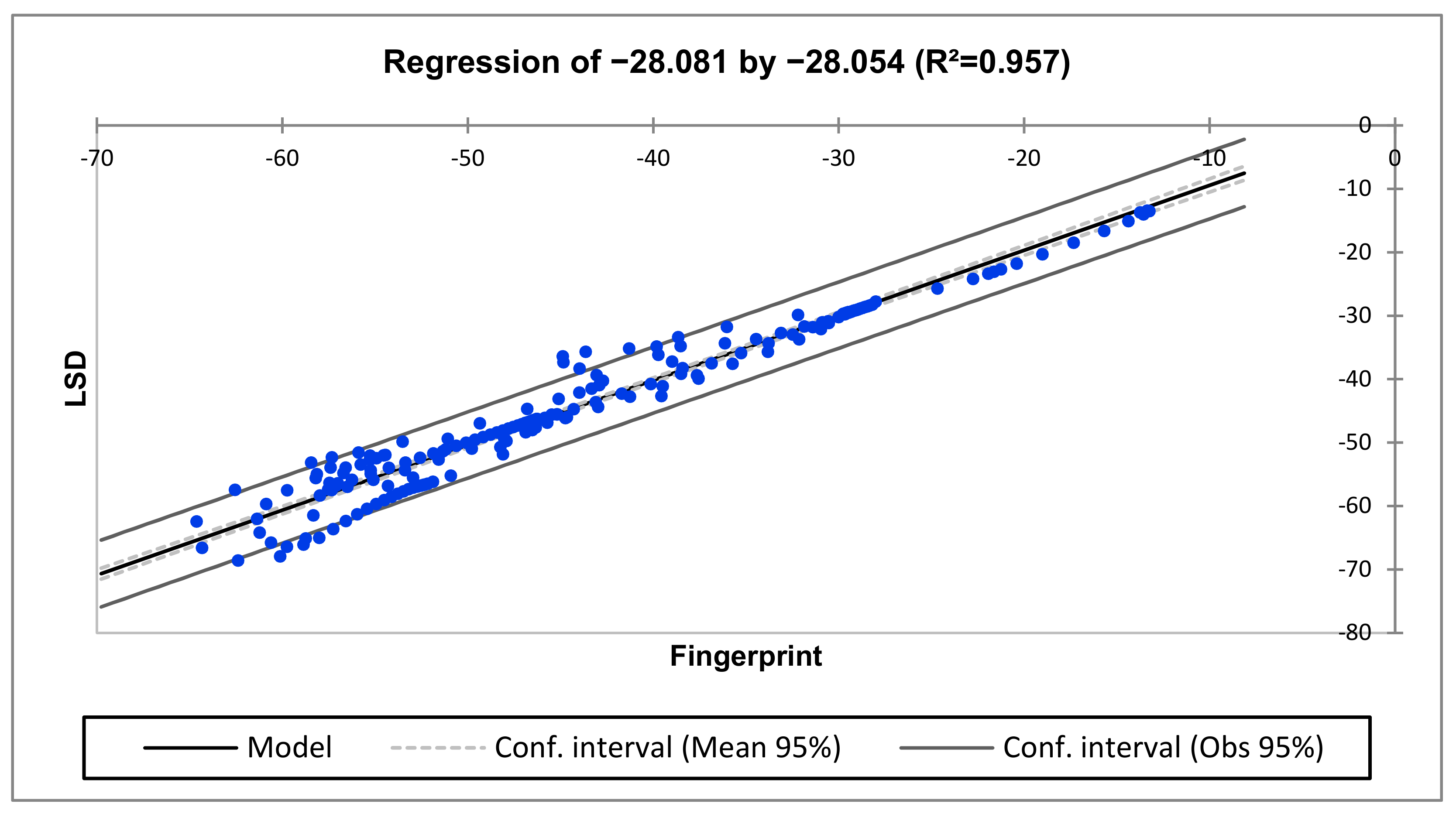
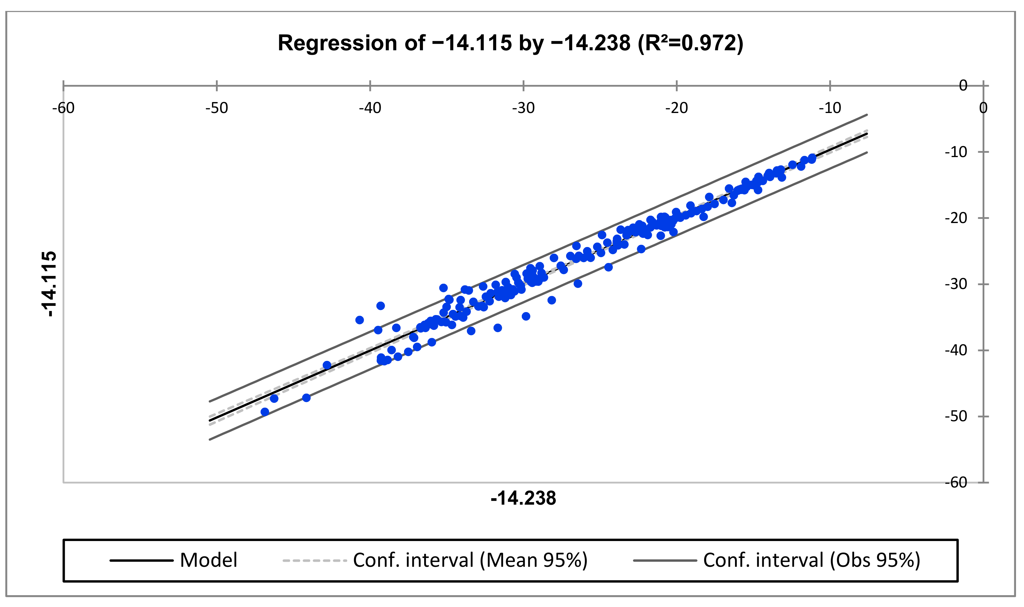
| R2 | 1.000 | 0.957 | 0.972 |
| Adjusted R2 | 1.000 | 0.957 | 0.972 |
Publisher’s Note: MDPI stays neutral with regard to jurisdictional claims in published maps and institutional affiliations. |
© 2022 by the authors. Licensee MDPI, Basel, Switzerland. This article is an open access article distributed under the terms and conditions of the Creative Commons Attribution (CC BY) license (https://creativecommons.org/licenses/by/4.0/).
Share and Cite
Thango, B.A.; Nnachi, A.F.; Dlamini, G.A.; Bokoro, P.N. A Novel Approach to Assess Power Transformer Winding Conditions Using Regression Analysis and Frequency Response Measurements. Energies 2022, 15, 2335. https://doi.org/10.3390/en15072335
Thango BA, Nnachi AF, Dlamini GA, Bokoro PN. A Novel Approach to Assess Power Transformer Winding Conditions Using Regression Analysis and Frequency Response Measurements. Energies. 2022; 15(7):2335. https://doi.org/10.3390/en15072335
Chicago/Turabian StyleThango, Bonginkosi A., Agha F. Nnachi, Goodness A. Dlamini, and Pitshou N. Bokoro. 2022. "A Novel Approach to Assess Power Transformer Winding Conditions Using Regression Analysis and Frequency Response Measurements" Energies 15, no. 7: 2335. https://doi.org/10.3390/en15072335