Methane Concentration Prediction Method Based on Deep Learning and Classical Time Series Analysis

Abstract

Methane is one of the most dangerous gases encountered in the mining industry. During mining operations, methane can be broadly classified into three states: mining excavation, stoppage safety check, and abnormal methane concentration, which is usually a precursor to a gas accident, such as a coal and gas outburst. Consequently, it is vital to accurately predict methane concentrations. Herein, we apply three deep learning methods—a recurrent neural network (RNN), long short-term memory (LSTM), and a gated recurrent unit (GRU)—to the problem of methane concentration prediction and evaluate their efficacy. In addition, we propose a novel prediction method that combines classical time series analysis with these deep learning models. The results revealed that GRU has the least root mean square error (RMSE) loss of the three models. The RMSE loss can be further reduced by approximately 35% by using the proposed combined approach, and the models are also less likely to result in overfitting. Therefore, combining deep learning methods with classical time series analysis can provide accurate methane concentration prediction and improve mining safety.

1. Introduction

Methane is a common byproduct of the mining industry [1]. It remains trapped inside coal seams and is gradually released during mining. Methane leakage from the working face can lead to asphyxiation, fire, coal and gas outbursts, and other accidents [2]. In the first half of 2021, there were several accidents caused by high methane concentrations [3] in various mines across China. These accidents led to severe injuries, high casualty rates, and considerable economic loss. Therefore, it is necessary to predict the methane concentration in mines efficiently and robustly, to prevent the occurrence of such accidents.

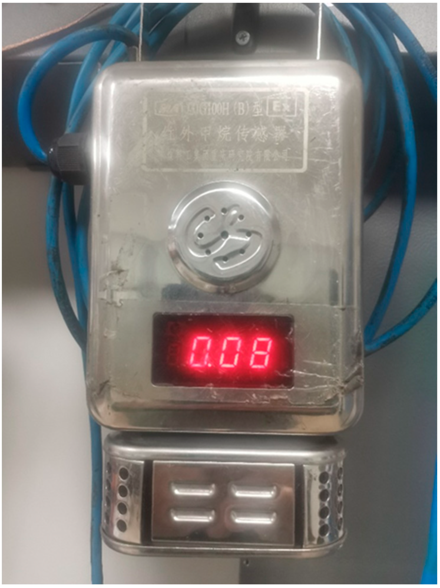
During mining, significant amounts of methane and other gases are released into the air from the working face [4,5]. Generally, numerous transducers are inserted in the working face of the mine to monitor various types of data, as shown in Figure 1, such as the methane concentration, temperature, wind speed, etc., in real time [6]. These sensor values are stored as time-series data that reflect the real-time situation of the mine. Analyzing this data can help prevent methane-related accidents.

Several researchers have studied the problem of methane release from working faces. Gao [7] used a combination of information fusion and chaotic time series analysis to predict gas emissions in tunnels. Zhang [8] developed a prediction model for coal-mine gas concentration using a time series and an adaptive neuro-fuzzy inference system (ANFIS). Fu [9] proposed a dynamic fuzzy neural network (IGA-DFNN) method optimized with an immunogenetic algorithm to accurately predict the gas concentration in coal seams. Karacan [10] proposed principal component analysis (PCA) and an artificial neural network (ANN)-based approach to predict the methane ventilation emission rates from US longwall mines. Yang [11] constructed a multivariate time series prediction model based on massive coal-mine gas monitoring data and a multivariate distribution lag model. Yang [12] developed a hybrid prediction model incorporating the wavelet transform and an extreme learning machine (ELM), Their proposed method is referred to as wavelet-based ELM (WELM) and is intended for predicting coal-mine gas concentrations. Zhang [13] used a pattern recognition method to predict the sub-unit probability of coal seam protrusion hazards and classified the coal and gas outburst levels of coal seams into three zones—the danger zone, threat zone, and safety zone. Dong [14] proposed a new coal and gas outburst prediction model based on the mechanism of the occurrence of coal and gas protrusions, related to coal strength, gas pressure, and in situ stress. Li [15] proposed a novel model based on multi-source information fusion to predict sudden-onset coal and gas disasters. Li [16] proposed a risk assessment of gas explosions based on fuzzy AHP and a Bayesian network.

Although these studies have resulted in significant advances and provided a reference for subsequent studies, the suggested methods have certain limitations. There are several aspects of methane concentration data that can influence the accuracy of methane prediction:

(1)

The transducers at the working face do not collect data at even time intervals. Some transducers record data once every minute, whereas others record data ten times a second.

(2)

The transducers need to be adjusted at regular intervals, and other human factors can also affect the acquisition of data, which can lead to sudden variations in the recorded data.

(3)

Each transducer can record vast amounts of data over a few months, which can translate to millions of pieces of data for the entire working face.

Traditional statistical models, such as the autoregressive integrated moving average model (ARIMA) [17], can be overwhelmed by the large volume of generated data and face problems related to the accuracy and robustness of the model and its generalization to different mines.

Deep learning is a relatively new technique that offers significant potential in addressing these problems. As deep learning is highly flexible, it allows the model to handle high-dimensional nonlinear problems without the need to ascertain the model parameters in advance. Consequently, deep learning models, such as recurrent neural network (RNN)-based models [18], offer several advantages when addressing methane concentration prediction problems. Song [19] constructed an RNN-based multi-parameter fusion prediction model for coal-seam gas concentration to improve the accuracy of gas concentration prediction. Lyu [20] proposed a multi-step prediction method for a gas concentration time series based on the ARMA, CHAOS, and encoder–decoder models (single-sensor and multi-sensor). Zhang [21] proposed a long short-term memory (LSTM) RNN prediction method, based on actual coal-mine production monitoring data, to effectively reduce the prediction error. Li [22] predicted the hazard potential of coal and gas outbursts using neural networks and clustering algorithms. Jia [23] proposed a gated recurrent unit (GRU)-based coal-mine gas concentration prediction model. The proposed model not only has a simple structure but also offers a high prediction accuracy and can make full use of the time series characteristics of coal-mine gas concentration data. In recent years, several deep learning-based models have been developed to analyze methane concentration data and the impact on mining safety as they are more sophisticated, can handle non-linear data, and can fit methane concentration trends.

Data play an increasingly important part in mining practice, with dozens of sensors in a single working face monitoring various features such as gas concentration, wind speed, temperature, carbon monoxide concentration, etc. Those data are stored as a time series; analysis of these data can uncover a variety of characteristics and achieve meaningful results, such as in [24], where the simulation of gas contamination of groundwater in mining excavations allows us to address environmental issues such as the groundwater-quality impacts of oil and gas extraction [25].

In this study, we combine deep learning with a traditional time series analysis method to train and evaluate multiple RNN-based models, namely, a classical RNN [18], LSTM [26], and GRU [27]. The data used to train the models were obtained from real working face sensors and were recorded over nearly three months. The performance of the models was evaluated through various experiments. Furthermore, we propose a novel approach that combines statistical analysis methods with deep learning to improve the prediction accuracy of the models. The efficacy of our proposed approach was evaluated experimentally, which can help build emergency plans [28] and reduce the probability of emergencies. By applying this research to a central server in an actual mine, we found that we could predict trends in methane concentration very well, which meant that we learned the inherent patterns of methane levels that can help us to identify potential gas accidents and improve mining safety.

2. Methods and Calculation

In this section, we describe the methods used herein, including those used to measure the performance of the models. Various forecasting and analysis methods, called time-series analyses [29], are used to predict methane concentrations in other fields. The process of analyzing these data requires expertise and the data must be suitably adjusted to achieve the best results.

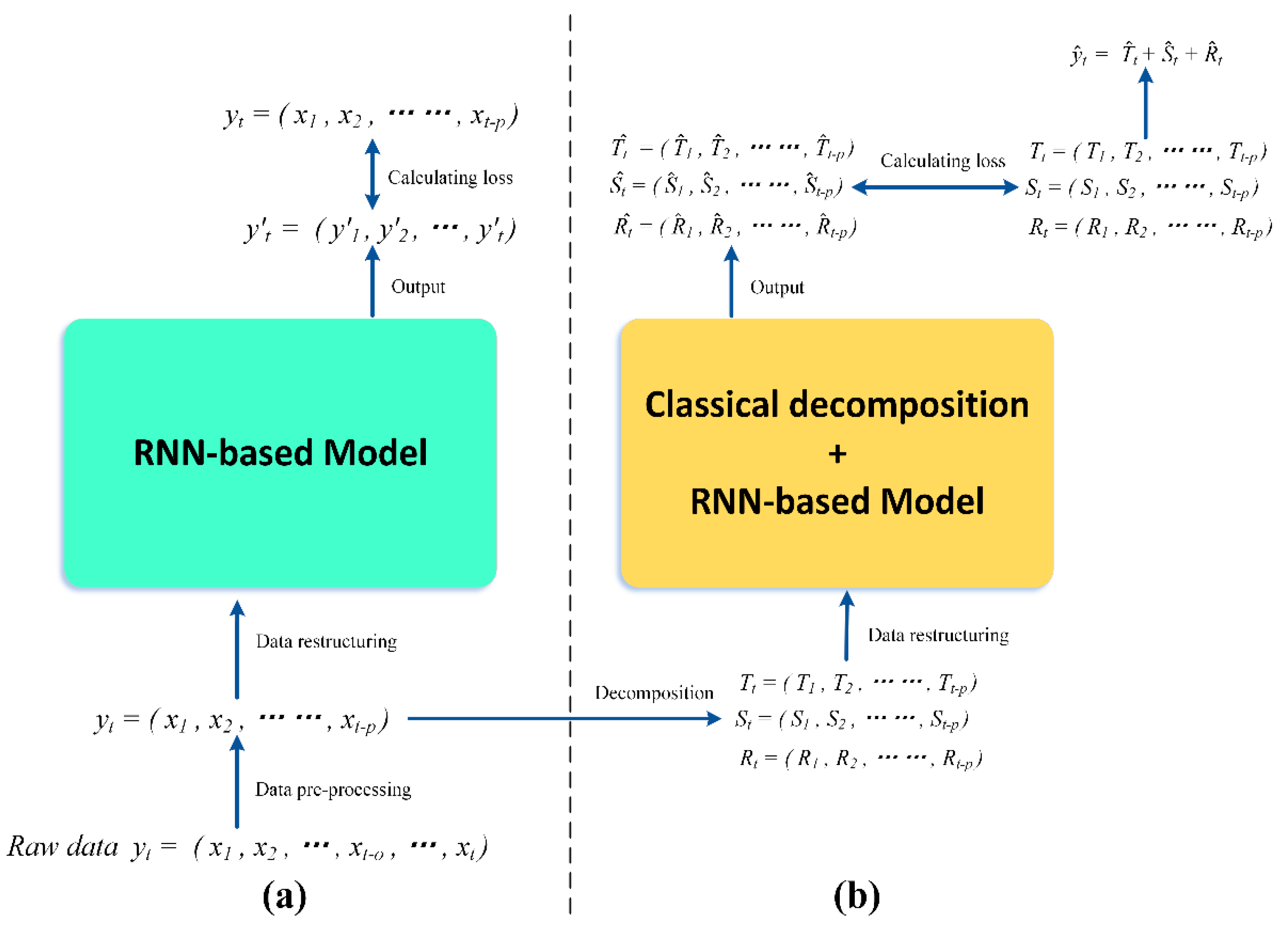
2.1. Classical Decomposition

Time series decomposition [30] is a classical time series analysis method that has two models: the additive decomposition model and the multiplicative decomposition model, which decomposes a time series $y_t$ into three components: the trend-cycle component, seasonal component, and remainder component [31]. The additive decomposition model can be expressed as:

$$y\left(t\right)=Trend\left(t\right)+Seasonal\left(t\right)+Remainder\left(t\right).$$

(1)

The multiplicative decomposition model can be expressed as:

$$y\left(t\right)=Trend\left(t\right)\times Seasonal\left(t\right)\times Remainder\left(t\right)$$

(2)

$$\log y\left(t\right)=\log Trend\left(t\right)+\log Seasonal\left(t\right)+\log Remainder\left(t\right).$$

(3)

As shown in Equation (3), the multiplicative model can be converted into an additive representation. The decomposition model provides an abstraction for analyzing the data and is suitable for prediction methods related to specific problems, such as methane concentration. The first step in the decomposition of time series data is to estimate the trend cycle using the moving averages method. A moving average of the order of $y_t$ can be expressed as:

$$T_t=\frac{1}{m}{\displaystyle \sum _{j=-k}^k{y}_t+j}$$

(4)

where $T_t$ is the trend and $m=2k+1$. That is, the estimate of the trend period in time $t$ is obtained by averaging the time series values over $k$ periods of time $t$. Thus, averaging removes some of the randomness from the data, leaving a smooth component of the trend cycle. This is referred to as $m--MA$, which denotes a moving average of order $m$. For additive decomposition, the general time series decomposition steps are as follows. (1) Seeking $T_t$: If the total length of the time series is even, $2\times m--MA$ (moving average) is used to calculate the trend; if the total length is odd, $m--MA$ is used to calculate the trend. (2) Determine the detrending series: $y\left(t\right)-T_t$. (3) Seeking $S_t$:$average\left(y\left(t\right)-T_t\right)$. (4) Seeking $R_t$: The remainder can be obtained by subtracting the seasonal and trend components from the series $R_t=y_t-S_t-T_t$.

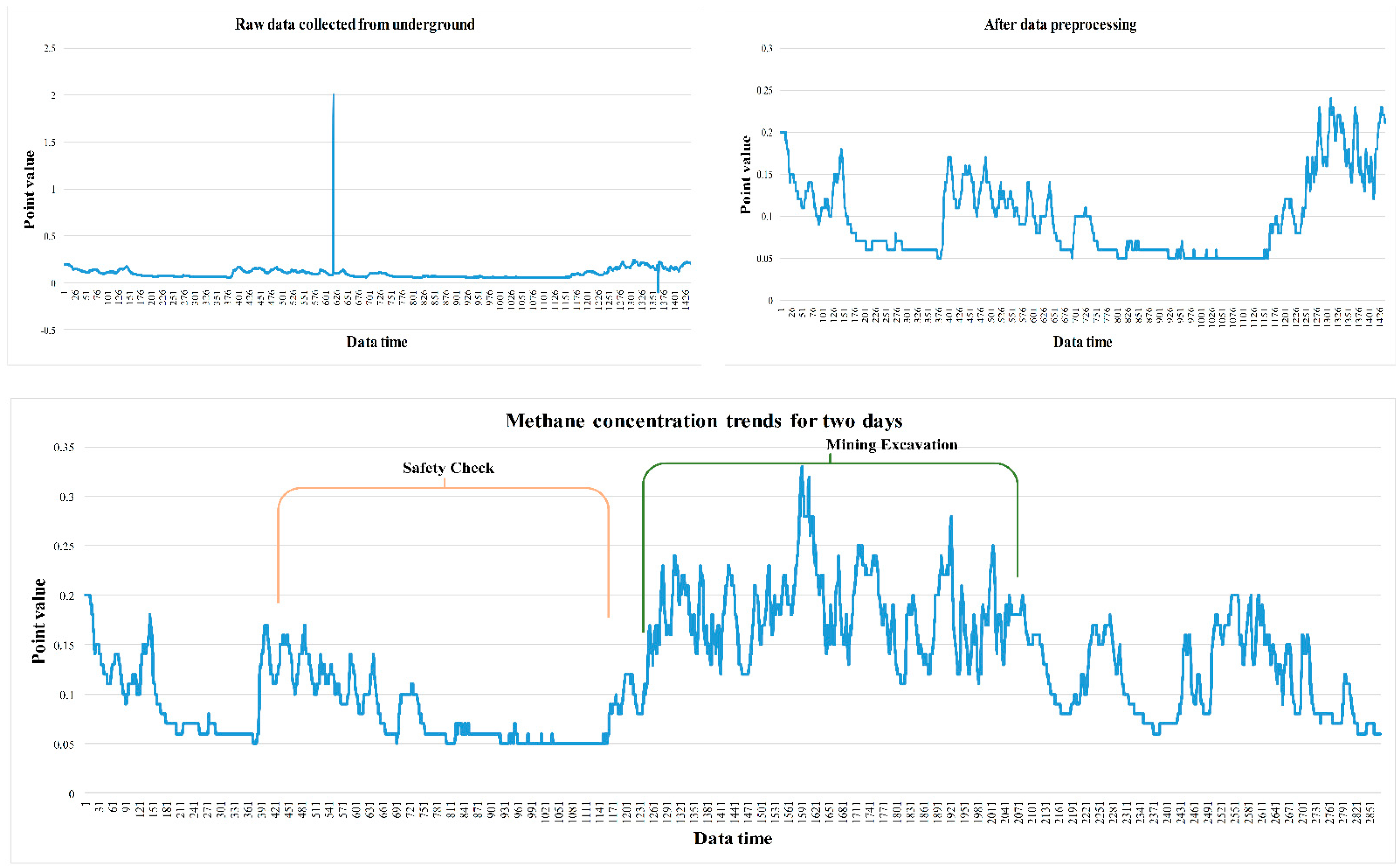
Multiplicative decomposition is similar to additive decomposition, except that addition and subtraction are replaced by multiplication and division. Classical decomposition is relatively easy and intuitive, but crucially, it provides unique and extremely useful a priori knowledge for building complex models such as deep neural networks and for dealing with non-linear data. This is particularly true for data that are clearly cyclical in nature, such as the methane released from the working face, which is characterized by a zig-zag increase during mining operations [32] and a gradual decrease during stoppages for safety checks, as shown in Figure 2.

The transducers in the working face must be calibrated regularly. Figure 2 illustrates the changes in methane values on the day of the calibration. As shown, the values at calibration point 2 are significantly higher than those normally acquired by the transducer, which affects the data analysis process. Figure 2 illustrates the methane concentration trend after data pre-processing and shows the methane concentration over two days. Mining activities are performed on a shift-work schedule, which includes regular stoppages in the work to perform various safety checks and remove any potential safety hazards. Consequently, methane levels gradually decrease during the safety checks and increase in a zig-zag manner when work restarts. The work schedule provided by the Qianyingzi coal mine confirms this trend.

Although some understanding of the general data trend is required to make forecasts using time series decomposition, there are obvious drawbacks to this approach: (1) estimates of the trend period for the first and last few observations are not available—that is, some values will inevitably be dropped to obtain a moving average; (2) estimates of trend cycles tend to smooth over sudden changes in the data; (3) the classical decomposition method assumes that the seasonal component repeats itself annually—although this is a reasonable assumption for several time-series data types, it does not apply to longer time-series data, such as the methane released from mines during the year (tens of billions of data points).

2.2. Deep Learning Models

Deep learning models have evolved rapidly in recent years and have achieved excellent results in many areas, such as computer vision (CV) [33], natural language processing (NLP) [34], and autopilot systems [35]. Consequently, the application of deep learning methods to methane prediction has good potential.

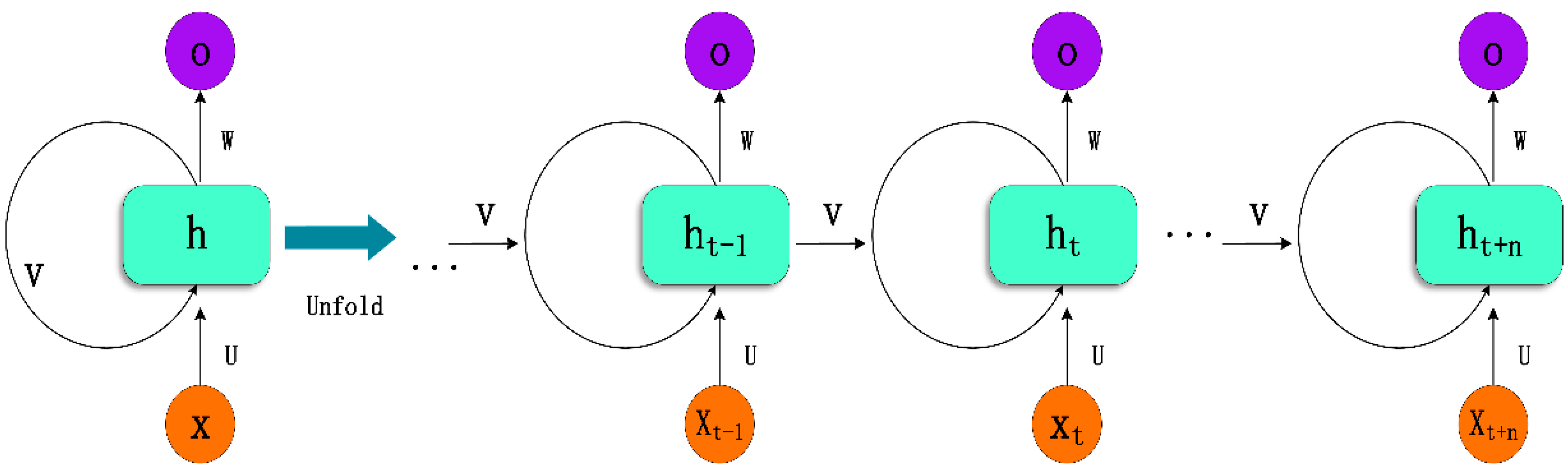
An RNN model, as shown in Figure 3, is a cell-based neural network, wherein each cell comprises three parts: an input layer, a hidden layer, and an output layer. The result of the output layer is determined not only by the input $X$ or the weights $W$ but also by the previous input $X_{t-1}$ and the previous weights. The output is controlled by an activation function and is connected by the weights between cells. The parameters are updated by a backpropagation through time algorithm for each calculation, which can be expressed as:

$$\begin{array}{l}{h}_t={\sigma }_h(W_h{x}_t+U_h{h}_{t-1}+b_h)\\ y_t={\sigma }_y(W_y{h}_t+b_y)\end{array}$$

(5)

where $x_t$ and $y_t$ are the input and output, $h_t$ is the hidden layer vector, and $W$, $U$, and $b$ are the weights between the input and hidden layers. The advantages of an RNN are: 1) they are specifically designed to handle time-series data, as the weight of the previous time affects the subsequent time, and the data in the time series are correlated in time; 2) theoretically, RNNs can simulate infinite stacks through activation and weighting; 3) RNNs allow complex nonlinear relationships and high dimensionality between the response variables; 4) compared to traditional models, RNNs do not require parameters to be determined in advance as the parameters are calculated in the model itself through backpropagation [36].

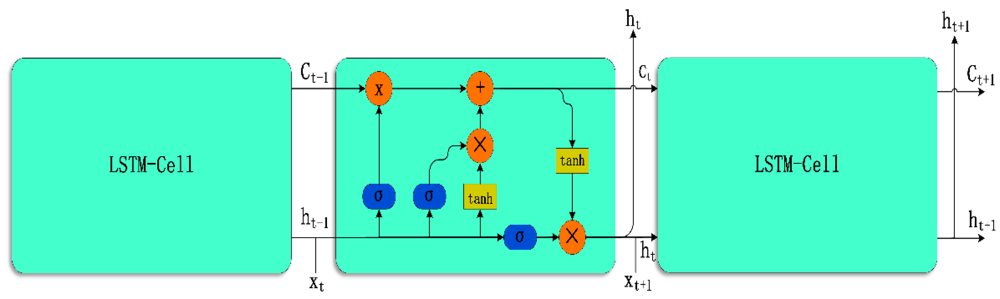
The short-term memory of a classical RNN is a double-edged sword, and the problems of vanishing [37] and exploding gradients often occur during model training [38]. Consequently, superior RNN models, such as the long short-term memory (LSTM) model, have been developed. LSTM is a special type of RNN that is primarily used to solve the problem of vanishing and exploding gradients while training long sequences. LSTM performs better in longer sequences compared to ordinary RNNs. The LSTM model can be expressed as:

$$\begin{array}{l}{f}_t={\sigma }_g(W_f{x}_t+U_f{h}_{t-1}+b_f)\\ i_t={\sigma }_g(W_i{x}_t+U_i{h}_{t-1}+b_i)\\ o_t={\sigma }_g(W_o{x}_t+U_o{h}_{t-1}+b_o)\end{array}$$

(6)

where $f_t$, $i_t$, and $o_t$ are the forget gate, input gate, and output gate, as shown in Figure 4; $W\in {ℝ}^{h\times d},U\in {ℝ}^{h\times h},b\in {ℝ}^h$ are the matrices for storing the weights in the training model; $x_t$ is the input; $h_t$ is the hidden state; and ${\sigma }_g$ and ${\sigma }_h$ denote the sigmoid and tan h functions, respectively. In the forget gate, the previous hidden state, which is a sigmoid function, enters the gate together with the current input. The closer the result is to 1, the greater its importance, and the closer it is to 0, the greater the need for it to be forgotten, thereby achieving the function of the forget gate. The LSTM parameters can be updated as:

$$\begin{array}{c}{c}_t=f_t\cdot c_{t-1}+i_t\cdot {\sigma }_c(W_c{x}_t+U_c{h}_{t-1}+b_c)\\ h_t=o_t\times {\sigma }_h(c_t)\end{array}$$

(7)

The most important function of these gates is to learn what is important and what is not important and needs to be dropped at a given moment in the time-series data. An unimportant input is never important, which is well suited to the prediction of methane concentration, as we wish to maximize the attention put on higher methane values such as 0.36 and 0.45, rather than on smaller values such as 0.01, 0.05, or even 0.

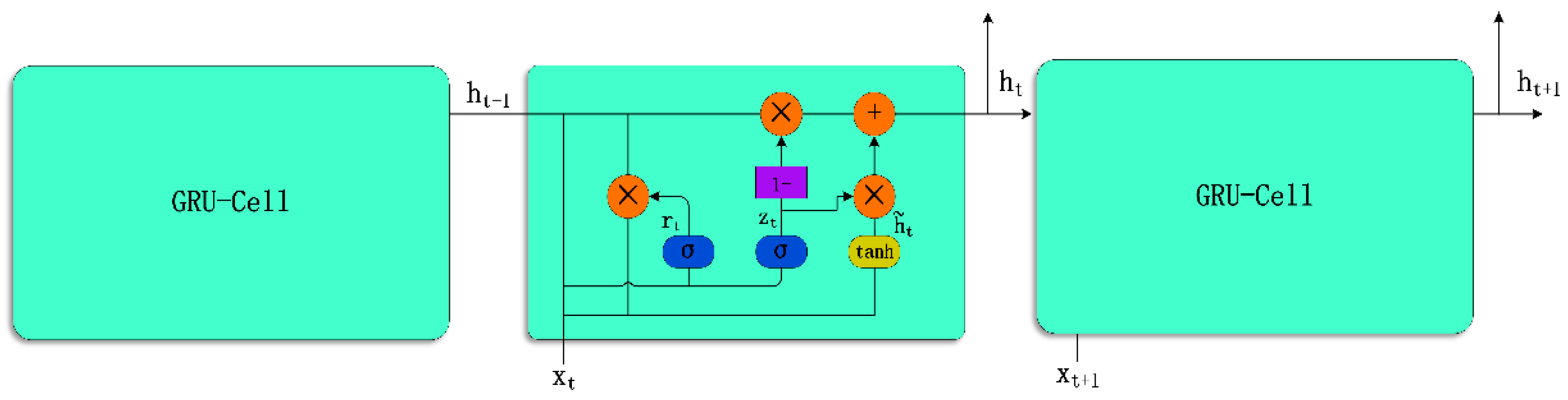
The GRU model is like an LSTM model with a forget gate, but has fewer parameters, such as the lack of an output gate, as shown in Figure 5. GRU outperforms LSTM on certain repetitive tasks such as tone music modeling, speech signal modeling, and natural language processing. However, although the performance of GRU is better than that of LSTM, it is relatively more time-consuming. In general, GRU can be expressed as:

$$\begin{array}{l}{z}_t={\sigma }_g(W_z{x}_t+U_z{h}_{t-1}+b_z)\\ {\gamma }_t={\sigma }_g(W_{\gamma }{x}_t+U_{\gamma }{h}_{t-1}+b_{\gamma })\\ {\widehat{h}}_t={\varphi }_h(W_h{x}_t+U_h({\gamma }_t{h}_{t-1})+b_h)\\ h_t=(1-z_t)h_{t-1}+z_t{\widehat{h}}_t\end{array}$$

(8)

where $x_t$ is the input vector, $z_t$ is the update gate vector, ${\gamma }_t$ is the reset gate vector, and $h_t$ and ${\widehat{h}}_t$ are the output and candidate activation vectors, respectively. In this study, we trained different RNN models using real-world methane data and measured their performance, considering loss, time complexity, and memory usage.

The developments in deep learning models have impacted various fields and have resulted in significant achievements. In coal mines, the significance of collecting and analyzing data from mines in real time is aided by information, pattern recognition, and trend prediction to ensure mine safety.

2.3. Loss Function and Optimization

The mean square error (MSE) is used as a metric in this study to measure the accuracy of the values predicted by the deep learning models compared to the actual methane concentration. MSE, which is also called the L2 loss function, optimizes the loss function for deep learning models by reducing its derivative to zero; it can also be used to evaluate the performance of the traditional model. MSE can be expressed as:

$$MSE=\frac{1}{n}{{\displaystyle \sum _{i=1}^n\left({\widehat{y}}_i-y_i\right)}}^2$$

(9)

MSE primarily calculates the error between the predicted value of the model and the true value. Another measure of the prediction accuracy is the root mean square error (RMSE), which is expressed as:

$$RMSE=\sqrt{\frac{1}{n}{{\displaystyle \sum _{i=1}^n\left({\widehat{y}}_i-y_i\right)}}^2}$$

(10)

The advantage of RMSE is that the calculated loss can be normalized to the predicted value, allowing a more intuitive view of the performance of the model. The correlation between the predicted and true values of methane can be measured using the coefficient of determination:

$$R^2=1-\frac{{\displaystyle \sum _i{({\widehat{y}}_t-y_t)}^2}}{{\displaystyle \sum _i{(y_t-\overline{y})}^2}}$$

(11)

where $y_t$ is the true value, and ${\widehat{y}}_t$ and $\overline{y}$ are the predicted value and the average of the true values, respectively.

The adaptive moment estimation (Adam) [39] is a deep learning model optimizer and represents an optimization of the stochastic gradient descent (SGD), which is widely used in computer vision and natural language processing. Combined with the momentum and root mean square propagation (RMSProp), Adam can be described as:

$$\begin{array}{c}{m}_{\omega }^{(t)}\leftarrow {\beta }_1{m}_{\omega }^{(t-1)}+\left(1-{\beta }_1\right){\nabla }_{\omega }{L}^{(t-1)}\\ {\widehat{m}}_{\omega }=\frac{m_{\omega }^{(t)}}{1-{\beta }_1^{t+1}}\end{array}$$

(12)

where $m_{\omega }^{(t)}$ is the first-order momentum and ${\beta }_1$ is the momentum factor. The concept of momentum is borrowed from physics; the true gradient is replaced by the previously accumulated momentum and $n_{\omega }^{(t)}$ is the second-order momentum:

$$\begin{array}{c}{n}_{\omega }^{(t)}\leftarrow {\beta }_2{n}_{\omega }^{(t-1)}+\left(1-{\beta }_2\right){({\nabla }_{\omega }{L}^{(t-1)})}^2\\ {\widehat{n}}_{\omega }=\frac{n_{\omega }^{(t)}}{1-{\beta }_2^{t+1}}\end{array}$$

(13)

The updated parameters can be expressed as:

$${\omega }^{(t)}\leftarrow {\omega }^{(t-1)}-\eta \frac{{\widehat{m}}_{\omega }}{\sqrt{{\widehat{n}}_{\omega }}+\epsilon }$$

(14)

where $\epsilon$ is a small value that prevents the gradient from being divided by zero. As an integrated optimization method, Adam offers many advantages: (1) simple and straightforward calculation; (2) efficiency; (3) reduced memory usage; (4) it is suitable for non-smooth targets; and (5) offers hyperparameters with intuitive interpretation. Therefore, it is well suited for optimizing the models used herein.

2.4. The Data

In this paper, the training data used to construct the deep learning models (RNN, LSTM, and GRU) were obtained from the methane sensors in the W3220 working face of the Qianyingzi coal mine in Suzhou, Anhui Province, China, and were recorded over nearly three months. The data were recorded from 1 May 2021 to 20 July 2021, with a total of 160,412 data points.

Our data comprise raw data extracted directly from the central server at the mine, which will then be deployed to the server to test the performance of the model once it has been trained.

3. Results

The values predicted by the RNN-based models can effectively fit the methane concentration data, but overfitting can occur in some cases. To prevent this, we use an early stop. After evaluating the performance of the three models, we propose a method that combines classical statistical analysis with deep learning models to further improve the prediction accuracy of the models and improve mining safety.

3.1. Development of an Accurate Methane Concentration Prediction Model

There are three steps in predicting methane concentration: data pre-processing, model construction, and model prediction. Data pre-processing is an essential and critical step as the real gas data or other data from the sensors cannot be directly analyzed by the algorithm owing to various factors, such as the manual adjustment of the sensors, sensor malfunctions that result in spikes or drops in the data values, missing segments, and negative values during the time period. Therefore, it is necessary to perform data cleaning, null data processing, feature extraction, and normalization, as shown in Figure 6a.

In Figure 6a, the raw data $y_t$ are preprocessed, wherein $x_{t-0}$ refers to outliers in the raw data such as calibration values, and $t-p$ denotes data that are pre-processed with the $p$ points deleted. After data pre-processing, the data are passed on to the reconstruction step, to train the RNN-based neural network model. A methane time series $y_t=x_1,x_2,\dots ,x_t$ is a time-ordered, limited fragment of unlimited sequences in time. A total of 160,412 pieces of data were used in the experiment. The data were obtained from the methane sensor in the upper corner of the working face of the Qianyingzi coal mine. The data were recorded from 1 May 2021 to 20 July 2021. To construct the dataset, we split $y_t$ into the training set $D_{train}=(x_1,x_2,\dots ,x_n)$ and the test set $D_{test}=(x_{n+1},x_{n+2},\dots ,x_m)$, in the ratio of $7:3$, where $t>m>n,(t,m,n)\in N$. The aim of this procedure is not only to train the RNN-based models with the temporal time-ordered property of the methane data $y_t$ but also to ensure that the data are linearly correlated within a certain time window. For example, herein, we chose 128 values of the methane data to represent the 129th value; we reconstructed the training set through a sliding window that can be represented as:

$$D_{train}=\{[X_1:(x_1,x_2,\dots ,x_{128}),Y_1:(x_{129})],[X_2:(x_2,x_3,\dots ,x_{129}),Y_2:(x_{130})],\dots ,[X_n:(x_{n+1},x_{n+2},\dots ,x_{n+127}),Y_n:(x_{n+128})]\}$$

(15)

After the dataset was reconstructed, we trained three RNN-based neural networks to determine the best model. Different batches and learning rates, such as $batch=[32,64,128]$ and $lr=[0.0001,0.0003,0.0005,0.0009,0.001]$, respectively, were chosen along with 30 epochs, with early stops for each model, to generate 15 results per model and 45 different results in total. MSE was used as the loss function and Adam was used as the optimizer of the neural networks. Considering model prediction, inserting the test dataset $D_{test}=(x_{n+1},x_{n+2},\dots ,x_m)$ into the model will output the predicted values ${y^{\prime }}_t=({y^{\prime }}_{n+1},{y^{\prime }}_{n+2},\dots ,{y^{\prime }}_m)$. Comparing the three RNN-based models—traditional RNN, LSTM, and GRU—we determined that the GRU model, with a batch size of 32 and a learning rate of 0.0005, provided the best performance. Out of a total of 45 models with approximately equal training times, six models with the least loss were selected, three of which were GRU models, as shown in Figure 7.

3.2. Improved Algorithm Combining Classical Decomposition and Deep Learning

Although deep learning models can effectively predict methane concentration, combining them with classical time series decomposition methods can further improve their prediction accuracy. The experiments performed herein indicate that the RMSE loss is reduced, and no overfitting occurs with this approach. However, the time required to train the model and the time requirements are increased.

Unlike the training procedure for the RNN-based neural network models discussed in Section 2, we first decompose the time series $y_t$ after obtaining the values of methane concentration at the upper corner (T0) of the working face, which gives us $T_t$, $S_t$, and $R_t$, based on Equation (1). For each component, the same RNN-based model is used to train and test the performance of the model using a test set. After the training is completed, three sets of predicted values are obtained, and separate predictions are made for each of the three decomposed components, as shown in Figure 6b. This gives us ${\widehat{T}}_t$, ${\widehat{S}}_t$, and ${\widehat{R}}_t$, which, when combined together, yield the new predicted values after RNN prediction:

$${\widehat{y}}_t={\widehat{T}}_t+{\widehat{S}}_t+{\widehat{R}}_t$$

(16)

where ${\widehat{T}}_t$, ${\widehat{S}}_t$, and ${\widehat{R}}_t$ are the trend, seasonality, and residuals predicted by the neural network, respectively. Adding these three vectors results in a smaller loss of ${y^{\prime }}_t$ than that predicted only with the neural network, as shown in Figure 8.

“Decomposition” in Figure 8 indicates that the methane time series is decomposed before training, whereas “solitary” indicates direct training. Decomposition refers to the time series decomposition of the methane concentration data to obtain the three components, which are then trained and predicted separately. The name solitary refers to the training and prediction of the pre-processed methane content values without any decomposition. It is more obvious that the predicted value of decomposition is closer to the true value in Figure 8. The results demonstrate that the decomposition prediction is better than the solitary prediction, in terms of both loss and decision coefficients. However, this improvement in performance occurs at the expense of computing time, to some extent.

3.3. Analysis of Results

The RNN-based models used herein are consistent, i.e., of 1 layer with 64 cells as the baseline model. The loss values using only the RNN-based deep learning models are shown in Figure 9, considering the performance of the three models under five learning rates and in three batches. As shown in Figure 9, for the classical RNN model, the best performance was achieved with slow learning rates and small batches. The LSTM model worked evenly across all cases. Although the GRU model was the best-performing model, it did not perform well with high learning rates.

The performance results of the combined decomposition and deep learning models are shown in Figure 10. The coefficients of determination, as shown in Figure 10a–c, represent the accuracy of the predicted values of the models compared to the true values, and should be as high as possible. A model with a learning rate of 0.0001 was used as a representative model to analyze the effect of different batch sizes on the model at the same learning rate. For the RNN models, the trend of the coefficient of determination changes consistently with the increase in batch size, with the decomposition method, and with the direct training method. For the LSTM models, the coefficient of determination increases with the increase in batch size, using the direct method. For the GRU models, the increase in batch size does not have a significant effect on the coefficients of determination of the model. However, the coefficient of determination using the decomposition method is higher than that of the direct training method, with values of more than 0.9. Thus, the predicted values are highly correlated with the true values.

The loss was evaluated using the RMSE loss. As shown in Figure 10d–f, the decomposition method had lower losses than the direct training method and improved the performance of all the models developed herein.

As discussed in Section 3.2, the decomposition approach decomposes the methane concentration $y_t$ into three parts, each of which trains the model separately. This triples the computational time in terms of the specification, as shown in Figure 11. The training time required for the decomposition method is three to four times greater than that required for the direct training method, which is a significant disadvantage of the decomposition method. However, for predicting methane concentration, the increase in training time is insignificant. Methane concentration has a clear trend, even if that trend is not evident to human observation. This trend can be learned by deep learning models. However, the pattern of methane concentration can change as mining progresses, as well as due to changes in the geological structure, coal seam content, excavation method, etc. In such cases, using previously recorded gas concentration data to predict the current data will result in poor accuracy and a large RMSE loss.

Based on the data used herein and our experience, it is best to use the methane concentration data of the previous three months for the real-time analysis of methane concentration, with approximately ten days of data being used as a test set to ensure the efficacy of the prediction model. The model should be retrained every month to ensure that it stays up to date with the underlying patterns of methane concentration. Notably, even the most time-consuming models do not require a training time of more than one hour. The time required to train the various models is illustrated in Figure 11.

As shown in Figure 11a–c, considering the solitary method, when the batch size is fixed, the time required to train the deep learning models does not change with the variation in the learning rate; when the learning rate is fixed, the time required to train the deep learning models decreases as the batch size increases. As shown in Figure 11d–f, these rules also apply to the decomposition method. Comparing Figure 11a–c with Figure 11d–f, respectively, it is evident that it takes three times longer to train the same parameters of the same model using the decomposition method, compared to the solitary method. This is because the decomposition method trains the trend, seasonal, and remainder components of the methane concentration separately.

4. Discussion

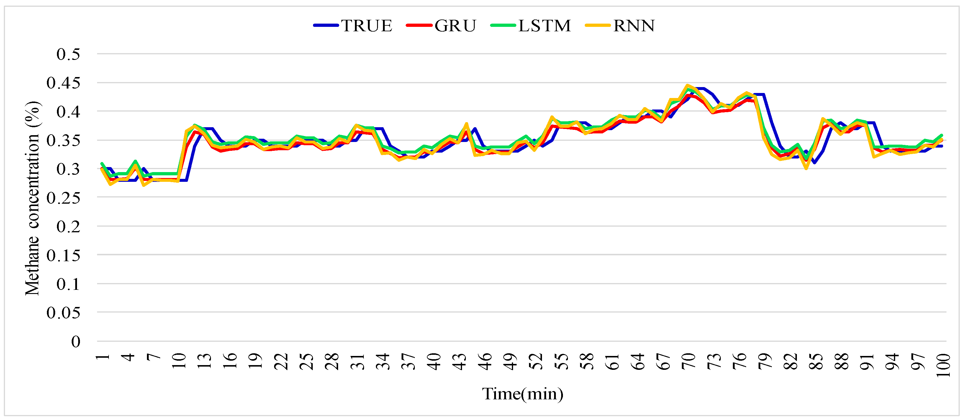
Methane concentration is an important consideration for ensuring the safety of coal mines as it has been known to cause hazardous accidents, such as coal and gas outbursts. Traditional methane-concentration prediction methods have encountered limitations in dealing with large data volumes and excessive dimensions. However, modern deep-learning approaches, such as RNN-based neural networks, can effectively solve these problems. Nonetheless, these advanced methods also face gradient and overfitting problems.

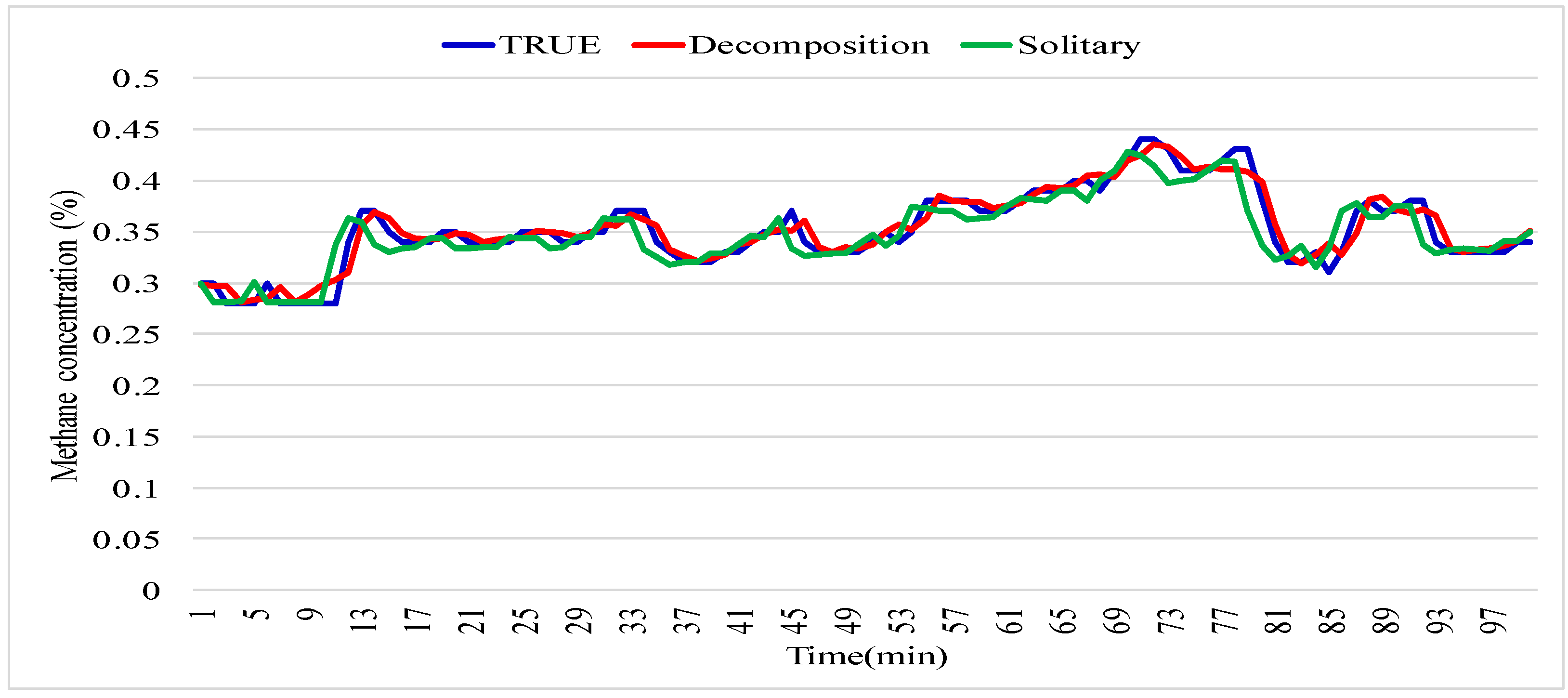
In this study, we employed three deep learning methods—RNN, LSTM, and GRU—to facilitate methane-concentration prediction and evaluated their efficacy. The experimental results obtained in this study reveal that the deep learning methods demonstrate great potential for use in applications related to ensuring mining safety. Moreover, it is observed that combining deep learning methods with classical time-series analysis approaches can further reduce the loss encountered by RNN-based models and improve the forecast accuracy. Unfortunately, this improvement in prediction accuracy is realized at the cost of an increased computational time because the combined approach takes approximately three times longer compared to pure RNN. However, the gas patterns in mine faces are never constant and change from one location to another as mining progresses. Therefore, gas-data sampling is limited to a few months rather than a few years, which reduces the computational burden. According to the Coal Mine Safety Regulations in China, the maximum methane concentration in the working face must not exceed 1%. This leads to an insignificant trend in methane concentration. Consequently, the application of deep-learning methods for ensuring the safety of coal-mining operations has become an important area of research in recent years. This means that we can systematically analyze the vast amount of underground data; learning the working patterns gives us the ability to recognize abnormal conditions, allowing us to detect and prevent catastrophic accidents in advance.

In future studies, we will analyze the correlation between transducers in the working face, such that even if one sensor fails, the methane concentration in the location of the failed sensor can be analyzed and predicted by the other transducers. This method can be used to analyze the change in methane concentration in mines where coal and gas outbursts have occurred. During coal and gas outburst accidents, the change in methane concentration differs from that recorded during normal operations. This change in methane concentration is either sudden or gradual but always occurs in a different pattern from that of the usual gas concentration, as demonstrated by the data obtained herein. Consequently, the deep learning methods proposed herein can provide an early warning of possible accidents, thereby improving mine safety and alleviating the loss of life.

5. Conclusions

In this study, three deep learning models were used to analyze and predict methane concentrations in underground mines using actual data recorded from the W3220 working face of the Qianyingzi coal mine in Suzhou, Anhui Province, China. The efficacy of the deep learning models was evaluated experimentally. In addition, we proposed a novel method that combines classical time series analysis with deep learning methods to predict methane concentration, which further reduces the RMSE loss. The effects of different hyperparameters on the accuracy of the deep learning models and the coefficient of determination were analyzed experimentally. The results demonstrated that deep learning methods can effectively predict methane concentration, and the proposed combined deep learning and traditional statistical method can further improve the prediction accuracy, although it is more time-consuming. In future studies, this method can be used to predict methane concentrations even when individual transducers fail, based on the trend data of the other transducers, which gives us the possibility of not only identifying accidents caused by methane but also can detect the accidents caused by worker mishandling, which is becoming a dominant factor in underground accidents. Therefore, deep learning methods can significantly improve the safety of underground mining.

References

1. Brodny, J.; Tutak, M. Analysis of methane hazard conditions in mine headings. Teh. Vjesn. 2018, 25, 271–276. [Google Scholar]
2. Felka, D.; Brodny, J. Application of neural-fuzzy system in prediction of methane hazard. In Proceedings of the Advances in Intelligent Systems and Computing, Lviv, Ukraine, 11–14 September 2018. [Google Scholar]
3. Xia, T.; Zhou, F.; Wang, X.; Zhang, Y.; Li, Y.; Kang, J.; Liu, J. Controlling factors of symbiotic disaster between coal gas and spontaneous combustion in longwall mining gobs. Fuel 2016, 182, 886–896. [Google Scholar] [CrossRef]
4. Karacan, C.Ö.; Ruiz, F.A.; Cotè, M.; Phipps, S. Coal mine methane: A review of capture and utilization practices with benefits to mining safety and to greenhouse gas reduction. Int. J. Coal Geol. 2011, 86, 121–156. [Google Scholar] [CrossRef]
5. Brodny, J.; Tutak, M. Analysis of methane emission into the atmosphere as a result of mining activity. In Proceedings of the International Multidisciplinary Scientific GeoConference Surveying Geology and Mining Ecology Management, SGEM, Albena Resort, Bulgaria, 28 June–7 July 2016. [Google Scholar]
6. Cao, J.; Li, W. Numerical simulation of gas migration into mining-induced fracture network in the goaf. Int. J. Min. Sci. Technol. 2017, 27, 681–685. [Google Scholar] [CrossRef]
7. Gao, L.; Yu, H.Z. Prediction of gas emission based on information fusion and chaotic time series. J. China Univ. Min. Technol. 2006, 16, 94–96. [Google Scholar]
8. Zhang, J.Y.; Cheng, J.; Hou, Y.H.; Bai, J.Y.; Pei, X.F. Forecasting coalmine gas concentration based on adaptive neuro-fuzzy inference system. Zhongguo Kuangye Daxue Xuebao/J. China Univ. Min. Technol. 2007, 36, 494–498. [Google Scholar]
9. Fu, H.; Li, W.; Meng, X.; Wang, G.; Wang, C. Application of IGA-DFNN for predicting coal mine gas concentration. Chin. J. Sens. Actuators 2014, 27, 262–266. [Google Scholar] [CrossRef]
10. Karacan, C.Ö. Modeling and prediction of ventilation methane emissions of U.S. longwall mines using supervised artificial neural networks. Int. J. Coal Geol. 2008, 73, 371–387. [Google Scholar] [CrossRef]
11. Yang, L.; Liu, H.; Mao, S.; Shi, C. Dynamic prediction of gas concentration based on multivariate distribution lag model. Zhongguo Kuangye Daxue Xuebao/J. China Univ. Min. Technol. 2016, 45, 455–461. [Google Scholar]
12. Xiang, W.; Jian-Sheng, Q.; Cheng-Hua, H.; Li, Z. Short-term coalmine gas concentration prediction based on wavelet transform and extreme learning machine. Math. Probl. Eng. 2014, 2014, 858260. [Google Scholar] [CrossRef]
13. Zhang, H.W.; Li, S. Pattern recognition and possibility prediction of coal and gas outburst. Yanshilixue Yu Gongcheng Xuebao/Chin. J. Rock Mech. Eng. 2005, 24, 3577–3581. [Google Scholar]
14. Dong, G.; Liang, X.; Wang, Q. A New Method for Predicting Coal and Gas Outbursts. Shock Vib. 2020, 2020, 8867476. [Google Scholar] [CrossRef]
15. Li, Y.; Yang, Y.; Jiang, B. Prediction of coal and gas outbursts by a novel model based on multisource information fusion. Energy Explor. Exploit. 2020, 38, 1320–1348. [Google Scholar] [CrossRef] [Green Version]
16. Li, M.; Wang, H.; Wang, D.; Shao, Z.; He, S. Risk assessment of gas explosion in coal mines based on fuzzy AHP and bayesian network. Process Saf. Environ. Prot. 2020, 135, 207–218. [Google Scholar] [CrossRef]
17. Hyndman, R.J.; Athanasopoulos, G. Forecasting: Principles and Practice. Princ. Optim. Des. OTexts 2018. [Google Scholar]
18. Rumelhart, D.E.; Hinton, G.E.; Williams, R.J. Learning representations by back-propagating errors. Nature 1986, 323, 533–536. [Google Scholar] [CrossRef]
19. Song, S.; Li, S.; Zhang, T.; Ma, L.; Pan, S.; Gao, L. Research on a multi-parameter fusion prediction model of pressure relief gas concentration based on RNN. Energies 2021, 14, 1384. [Google Scholar] [CrossRef]
20. Lyu, P.; Chen, N.; Mao, S.; Li, M. LSTM based encoder-decoder for short-term predictions of gas concentration using multi-sensor fusion. Process Saf. Environ. Prot. 2020, 137, 93–105. [Google Scholar] [CrossRef]
21. Zhang, T.; Song, S.; Li, S.; Ma, L.; Pan, S.; Han, L. Research on gas concentration prediction models based on lstm multidimensional time series. Energies 2019, 12, 161. [Google Scholar] [CrossRef] [Green Version]
22. Li, S.; Zhang, H.W. Pattern recognition and forecast of coal and gas outburst. J. China Univ. Min. Technol. 2005, 15, 251–254. [Google Scholar]
23. Jia, P.; Liu, H.; Wang, S.; Wang, P. Research on a Mine Gas Concentration Forecasting Model Based on a GRU Network. IEEE Access 2020, 8, 38023–38031. [Google Scholar] [CrossRef]
24. Taherdangkoo, R.; Yang, H.; Akbariforouz, M.; Sun, Y.; Liu, Q.; Butscher, C. Gaussian process regression to determine water content of methane: Application to methane transport modeling. J. Contam. Hydrol. 2021, 243, 103910. [Google Scholar] [CrossRef] [PubMed]
25. Taherdangkoo, R.; Tatomir, A.; Sauter, M. Modeling of methane migration from gas wellbores into shallow groundwater at basin scale. Environ. Earth Sci. 2020, 79, 432. [Google Scholar] [CrossRef]
26. Hochreiter, S.; Schmidhuber, J. Long Short-Term Memory. Neural Comput. 1997, 9, 1735–1780. [Google Scholar] [CrossRef]
27. Cho, K.; Van Merriënboer, B.; Gulcehre, C.; Bahdanau, D.; Bougares, F.; Schwenk, H.; Bengio, Y. Learning phrase representations using RNN encoder-decoder for statistical machine translation. In Proceedings of the EMNLP 2014–2014 Conference on Empirical Methods in Natural Language Processing, Doha, Qatar, 25–29 October 2014. [Google Scholar]
28. Onifade, M. Towards an emergency preparedness for self-rescue from underground coal mines. Process Saf. Environ. Prot. 2021, 149, 946–957. [Google Scholar] [CrossRef]
29. Berk, R.A.; McCleary, R.; Hay, R.A. Applied Time Series Analysis for the Social Sciences. Contemp. Sociol. 1981, 10, 818. [Google Scholar] [CrossRef]
30. West, M. Time series decomposition. Biometrika 1997, 84, 489–494. [Google Scholar] [CrossRef]
31. Mills, T.C. Applied Time Series Analysis: A Practical Guide to Modeling and Forecasting; Academic Press: Cambridge, MA, USA, 2019; ISBN 9788578110796. [Google Scholar]
32. Fan, C.; Li, S.; Luo, M.; Du, W.; Yang, Z. Coal and gas outburst dynamic system. Int. J. Min. Sci. Technol. 2017, 27, 49–55. [Google Scholar] [CrossRef]
33. Voulodimos, A.; Doulamis, N.; Doulamis, A.; Protopapadakis, E. Deep Learning for Computer Vision: A Brief Review. Comput. Intell. Neurosci. 2018, 2018, 7068349. [Google Scholar] [CrossRef]
34. Young, T.; Hazarika, D.; Poria, S.; Cambria, E. Recent trends in deep learning based natural language processing. IEEE Comput. Intell. Mag. 2018, 13, 55–75. [Google Scholar] [CrossRef]
35. Grigorescu, S.; Trasnea, B.; Cocias, T.; Macesanu, G. A survey of deep learning techniques for autonomous driving. J. Field Robot. 2020, 37, 362–386. [Google Scholar] [CrossRef]
36. Hecht-Nielsen, R. Theory of the Backpropagation Neural Network. Neural networks for perception; Academic Press: Cambridge, MA, USA, 1992; pp. 65–93. [Google Scholar]
37. Hochreiter, S. The vanishing gradient problem during learning recurrent neural nets and problem solutions. Int. J. Uncertain. Fuzziness Knowlege-Based Syst. 1998, 6, 107–116. [Google Scholar] [CrossRef] [Green Version]
38. Pascanu, R.; Mikolov, T.; Bengio, Y. On the difficulty of training recurrent neural networks. In Proceedings of the 30th International Conference on Machine Learning, ICML, Atlanta, GA, USA, 16–21 June 2013. [Google Scholar]
39. Kingma, D.P.; Ba, J.L. Adam: A method for stochastic optimization. In Proceedings of the 3rd International Conference on Learning Representations, ICLR 2015—Conference Track Proceedings, San Diego, CA, USA, 7–9 May 2015; pp. 1–15. [Google Scholar] [CrossRef]
Figure 1. Methane transducer.
Energies 15 02262 g001
Figure 2. Methane concentration trends.
Energies 15 02262 g002
Figure 3. RNN model.
Energies 15 02262 g003
Figure 4. LSTM model.
Energies 15 02262 g004
Figure 5. GRU model.
Energies 15 02262 g005
Figure 6. Comparison of two methane concentration prediction methods. (a) is RNN-based Model only and (b) is RNN-based optimization model based on time series Classical decomposition methods.
Energies 15 02262 g006
Figure 7. Comparison between methane concentration predictions obtained using three RNN-based models.
Energies 15 02262 g007
Figure 8. Comparison between methane concentration predictions obtained using decomposition and direct prediction methods.
Energies 15 02262 g008
Figure 9. RMSE loss of the three models.
Energies 15 02262 g009
Figure 10. Determination coefficients and RMSE losses with the two prediction methods for the three RNN-based models. (ac) and (df) are the coefficient of determination and RMSE loss under the same parameters of the model.
Energies 15 02262 g010
Figure 11. Comparative time consumption with the two methods. (a,d), (b,e), (c,f) are comparison of time consumption under the same parameter model respectively.
Energies 15 02262 g011
Publisher’s Note: MDPI stays neutral with regard to jurisdictional claims in published maps and institutional affiliations.