Article

Ensemble Learning-Based Reactive Power Optimization for Distribution Networks

1
School of Electrical Engineering, Tibet Agricultural and Animal Husbandry University, Linzhi 860000, China
2
Integrated Service Center of State Grid Tibet Electric Power Supply Company, Lhasa 850000, China
*
Author to whom correspondence should be addressed.
Energies 2022, 15(6), 1966; https://doi.org/10.3390/en15061966
Submission received: 15 February 2022 / Revised: 3 March 2022 / Accepted: 7 March 2022 / Published: 8 March 2022

Abstract

:
Reactive power optimization of distribution networks is of great significance to improve power quality and reduce power loss. However, traditional methods for reactive power optimization of distribution networks either consume a lot of calculation time or have limited accuracy. In this paper, a novel data-driven-based approach is proposed to simultaneously improve the accuracy and reduce calculation time for reactive power optimization using ensemble learning. Specifically, k-fold cross-validation is used to train multiple sub-models, which are merged to obtain high-quality optimization results through the proposed ensemble framework. The simulation results show that the proposed approach outperforms popular baselines, such as light gradient boosting machine, convolutional neural network, case-based reasoning, and multi-layer perceptron. Moreover, the calculation time is much lower than the traditional heuristic methods, such as the genetic algorithm.

1. Introduction

Reactive power optimization is one of the widely used means to reduce power loss and improve power quality by regulating the state of equipment, such as shunt capacitor bank, on-load tap changer (OLTC), and static var compensator (SVC). As a crucial component of the planning and scheduling of distribution networks, reactive power optimization is of great importance for both practical engineering and theoretical study [1].
Traditional methods of reactive power optimization can be subsumed under just two categories: heuristic algorithms [2] and mathematical programming algorithms [3]. Specifically, mathematical programming algorithms mainly consist of dynamic programming, linear programming, and non-linear programming. Although these mathematical programming algorithms have low complexity and fast computational speed, they have difficulty in dealing with non-linear and high-dimensional reactive power optimization problems, which results in limited optimization accuracy. The popular heuristic algorithms mainly include particle swarm optimization (PSO), simulated annealing (SA), and genetic algorithm (GA). Despite these heuristic algorithms significantly outperforming mathematical programming algorithms in terms of optimization accuracy, they involve heavy computational burdens, especially for large-scale distribution networks [4]. Therefore, it is necessary to develop a new method with a fast computational speed and high accuracy.
Driven by the development of smart meters, sensors, and communication technologies, the historical data stored in supervisory control and data acquisition systems show explosive growth, which brings opportunities to the application of data-driven technology in reactive power optimization. The existing data-driven-based algorithms for reactive power optimization can be subsumed under just two categories: similarity-based algorithms [5] and model-based algorithms [6]. Specifically, similarity-based algorithms mainly consist of case-based reasoning (CBR), expert systems, Apriori algorithms, and large random matrix theory, which intend to calculate distances between historical cases and new cases [7]. However, it is inappropriate to assign the strategy of historical cases to new cases directly, especially when the current load distribution is significantly different from the historical load distribution. For model-based algorithms, they mainly include light gradient boosting machine (LightGBM), multi-layer perceptron (MLP), convolutional neural network (CNN), etc. Specifically, these model-based algorithms use models (e.g., deep neural networks) to project the non-linear relationship between power loads (e.g., active power and reactive power) and dispatching strategies, and their accuracy is higher than those of similarity-based algorithms, especially when the power loads change dramatically. While these model-based algorithms can be effective reactive power optimization, each has its own advantages and disadvantages, limiting its accuracy in the application of reactive power optimization.
Ensemble learning employs multiple models to achieve better performance than could be obtained from any of the constituent models alone. Up to now, ensemble learning has shown convincing performance in classification, function approximation, prediction, etc. [8]. Reactive power optimization of distribution networks can be regarded as a special regression problem, projecting the relationship between power loads and dispatching strategy through different models. Therefore, ensemble learning should have the potential for reactive power optimization of distribution networks. In [9,10], ensemble learning is used to estimate the linear power flow of distribution networks. In other words, these previous publications employ ensemble learning to map the non-linear relationship between the magnitude and phase angle of voltage and power loads. They can only be used to obtain the power flow of distribution networks and cannot provide guidance for the operation state of the power equipment to achieve the optimal power flow.
Further, this paper focuses on how to apply ensemble learning to obtain the optimal dispatching strategy for the reactive power optimization task of distribution networks, namely, the application of ensemble learning in optimal power flows. Compared with previous publications [9,10], the proposed method is concerned with optimal power flows rather than simple power flow calculations. The key contributions are summarized as follows:
(1)
A fully data-driven and scalable method is proposed for reactive power optimization of distribution networks without solving complex physical models. Additionally, the proposed approach is applied to different distribution networks by simply fine-tuning the structures and parameters.
(2)
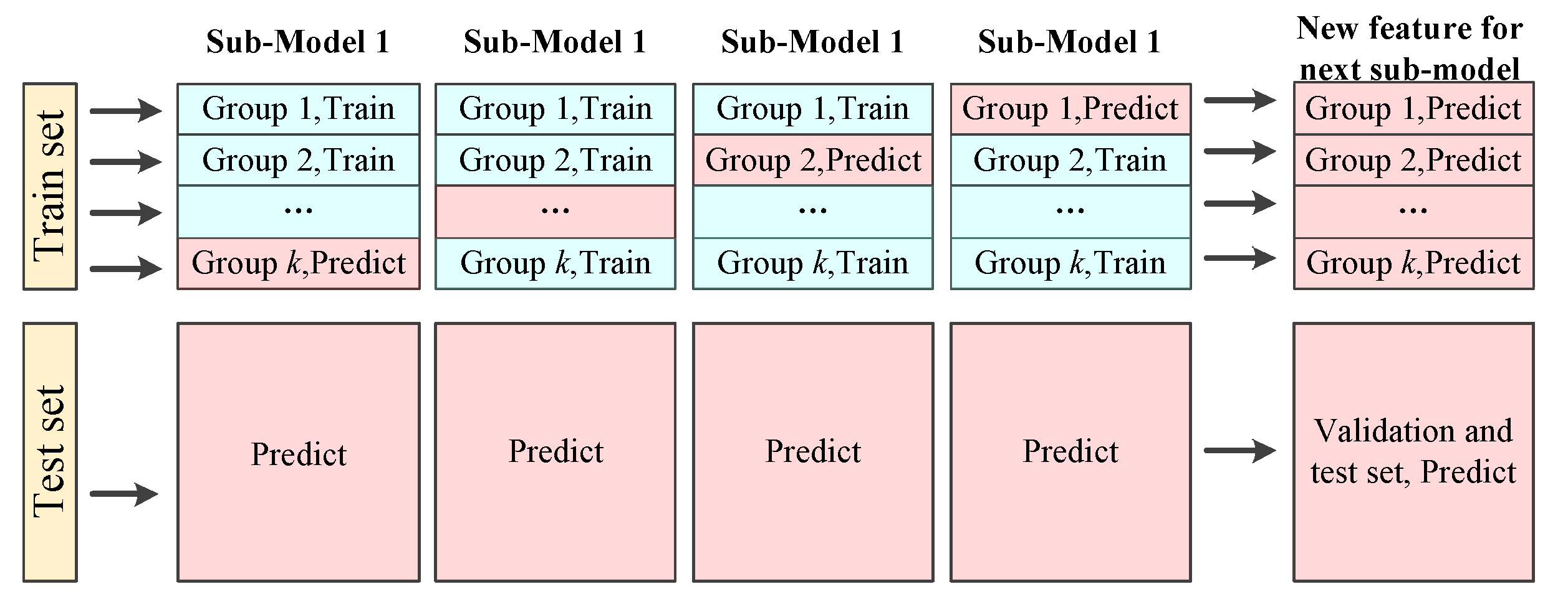
Each method has its own advantages and disadvantages, while the proposed approach can learn widely from others’ strong points to improve the optimization accuracy. To improve the generalization of the ensemble model, k-fold cross-validation is employed to train the model.
(3)
Numerical experiments on the real-world dataset are performed to validate the effectiveness of the ensemble framework for reactive power optimization of distribution networks. The simulation results show that the proposed approach achieves state-of-art performance with superior accuracy. Further, the calculation time is much lower than the traditional heuristic methods, such as GA.
The rest of this paper is organized as follows: Section 2 formulates the reactive power optimization model. Section 3 describes the application of ensemble learning in reactive power optimization. Simulations and results are discussed in Section 4. Section 5 summarizes the conclusions.

2. Reactive Power Optimization Model

Normally, the goal of reactive power optimization is to reduce power loss and improve the power quality of distribution networks [11]. Without loss of generality, the changes of power loss and voltage offset are defined as a comprehensive objective function of reactive power optimization in this paper:
max F 1 = W P loss P loss P loss + ( 1 W ) d U d U d U
d U = i = 1 n | U 0 U i U 0 |
P loss = l = 1 N R l P l 2 + Q l 2 U l 2
where W is the weight (i.e., W is 0.5 in this paper), which is used to balance the power loss and voltage offset; P loss is the power loss before reactive power optimization; P loss is the power loss after reactive power optimization; d U is the voltage offset before reactive power optimization; d U is the voltage offset after reactive power optimization; n is the number of nodes in distribution networks; N is the number of branches in distribution networks; U 0 is the rated voltage; U i is the voltage of node i ; R l is the resistance of branch l; P l is the active power of terminal node in the branch l ; Q l is the reactive power of terminal node in the branch l; and Ul is the voltage of terminal node in the branch l .
Additionally, the reactive power optimization model of distribution networks has to meet the following constraints:
(1)
Power flow constraints in distribution networks
{ P i U i j = 1 n U j ( G i j cos δ i j + B i j sin δ i j ) = 0 , i = 1 , 2 , n Q i U i j = 1 n U j ( G i j sin δ i j B i j cos δ i j ) = 0 , i = 1 , 2 , n
where δ i j is the phase difference of the voltage between node i and node j , G i j is the conductance between node i and node j , and B i j is the susceptance between node i and node j .
(2)
Current and voltage constraints in distribution networks
{ U i , min U i U i , max , i = 1 , 2 , n I l I l , max , l = 1 , 2 , N
where U i , max is the upper bound of voltage for node i , U i , min is the lower bound of voltage for node i , and I l , max is the upper bound of current for branch l .
(3)
Equipment constraints in distribution networks
{ 0 Q C i , t Q C , max , i = 1 , 2 , n C T i , min T i , t T i , max , i = 1 , 2 , n T 0 Q SVC i , t Q SVC , max , i = 1 , 2 , n S V C
where n C is the number of nodes with the shunt capacitor bank, n T is the number of nodes with OLTC, n S V C is the number of nodes with SVC, Q C , max is the maximum reactive power generated by the shunt capacitor bank, T i , min is the minimum tap position of the OLTC, T i , max is the maximum tap position of the OLTC, and Q SVC , max is the maximum reactive power generated by the SVC.
Moreover, different sub-models (i.e., neural networks) are used to project the complex relationship between power loads and dispatching strategy. The new form of the comprehensive objective function can be defined as its opposite. Considering that these sub-models are difficult to deal with constraints directly, the penalty function method is employed to transform the reactive power optimization model into an unconstrained optimization problem.
max F 2 = F 1 λ 1 i = 1 n [ ε ( U i U i , max ) + ε ( U i , min U i ) ] λ 2 l = 1 N ε ( I l I l , max )
where F 2 is a new form of the comprehensive objective function, λ 1 is the penalty coefficient of voltage constraints, ε is the step function, and λ 2 is the penalty coefficient of current constraints.
Note that dynamic reactive power optimization has the third constraint, while static reactive power optimization does not need to consider them. In this paper, the time interval control strategy is used to divide a day into several time intervals [12]. Then, the dynamic reactive power optimization is simplified to multiple static reactive power optimizations within the interval. Therefore, the third constraint was not added to the comprehensive objective function, since they have been implicitly considered by the time interval control strategy.

3. Methodology

3.1. Framework of the Proposed Method

Ensemble learning is a popular meta approach of machine learning that obtains strong performance by combining the forecasting results from multiple different sub-models [13]. As one of the contributions of this paper, this section presents a framework that can ensemble three popular sub-models to obtain dispatching strategies of reactive power optimization, as shown in Figure 1.
First of all, the power loads are regarded as original features to train Model 1, which outputs the forecasting values (i.e., dispatching strategy). The power loads and the predicted dispatching strategy of distribution networks are considered as new input features of the next sub-model. Then, the new input features are used to train Model 2, which predicts the dispatching strategy of the training set and test set. The power loads, the predicted dispatching strategy of Model 1 and Model 2 are considered as new input features for the next sub-model. Similarly, the new input features are used to train Model 3, which predicts the dispatching strategy of the test set. Finally, final results can be obtained by averaging forecasting values of all sub-models.
Traditional hold-out validation is dependent on just one train-test split, which makes its performance depend on how the data are divided into the training set and test set. Relatively, k-fold cross-validation is a popular resampling technique, which is widely used to improve the generalization of different models in computer visions [14]. The technique has a single parameter k, which refers to the number of groups that a given dataset is to be divided into. So far, k-fold cross-validation has shown outstanding performance for different fields such as classification and prediction tasks. As another contribution of this paper, k-fold cross-validation is generalized from computer vision into the training process of each sub-model for reactive power optimization. The specific framework is shown in Figure 2.
Firstly, samples in the training set are sectioned into k equal groups. The samples in the first k − 1 groups are used to train a sub-model, which predicts the dispatching strategies of samples in the kth group and test set. Secondly, the samples in the training set (except for samples in the (k − 1)th groups) are utilized to train a sub-model, which predicts the dispatching strategies of samples in the (k − 1)th group and test set. Similarly, k sub-models can be trained to predict the dispatching strategies of samples in the training set and test set. Finally, the predicted dispatching strategies of the training set are considered as a new feature, which is used to train the next sub-model, and the average values of the test set are the output results of this sub-model.
Compared with other data-driven-based methods, CNN, MLP, and LightGBM have better performance in many fields. Therefore, they are employed as examples to verify the effectiveness of the proposed ensemble framework [15]. Note that these three models may be replaced with other advanced models in future work. In the following sections, this paper shows how to employ sub-models to map the non-linear relationship between power loads and dispatching strategies, which is one of the contributions.

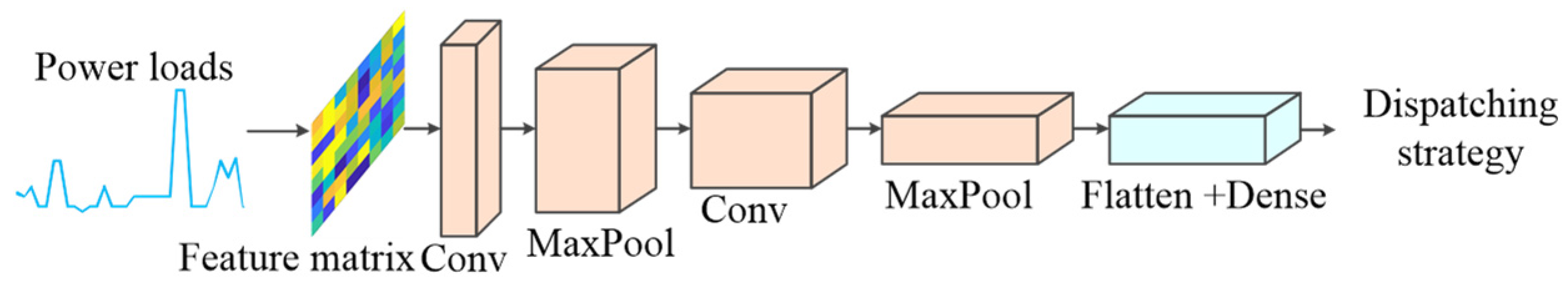
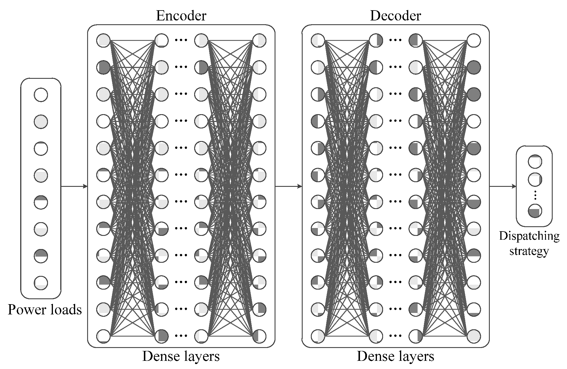
3.2. Convolutional Neural Network

The emergence of CNN has greatly promoted the development process of deep learning and artificial intelligence. So far, CNN has been widely used in various fields, such as target detection, fault diagnosis, time-series prediction, and semantic segmentation due to its powerful feature extraction capability [16]. As shown in Figure 3, a simple CNN structure consists of a convolutional layer, a pooling layer, and a dense layer.
Specifically, the convolutional operation is performed to extract features of input data, and then a bias vector is added to obtain the output data of convolutional layers:
Y con = σ con ( X con W con + B con )
where Y con is the output data of convolutional layers, X con is the input data of convolutional layers, σ con ( ) is the activation function of convolutional layers, W con represents weights of convolutional layers, and B con represents bias vectors of convolutional layers. Note that the output data of convolutional layers is utilized as the input data to the following maximum pooling layers.
As shown in Figure 4, the maximum pooling layer is employed to reduce the dimensionality of input data:
Y pool = max R ( X pool )
where Y pool is the output data of maximum pooling layers, X pool is the input data of maximum pooling layers, and R is the domain of definition for maximum pooling layers. Note that the output data of maximum pooling layers is utilized as the input data to the following convolutional layers or dense layers.
To reshape the multi-dimensional tensors into a one-dimensional vector, a flatten layer is inserted between dense layers and the last maximum pooling layer. Moreover, the vectors from the flatten layer are fed to a dense layer to obtain dispatching strategies:
Y dense = σ dense ( X dense W dense + B dense )
where Y dense is the output data of dense layers, X dense is the input data of dense layers, σ dense ( ) is the activation function of dense layers, W dense represents weights of dense layers, and B dense represents bias vectors of dense layers.

3.3. Multi-Layer Perceptron

Normally, the MLP consists of multiple dense layers. In this paper, the encoder–decoder pipeline is used to project the non-linear relationship between power loads and dispatching strategies, as shown in Figure 5.
For the encoder, low-dimensional latent variables can be obtained by feeding input data to multiple dense layers:
Y en = σ en ( X en W en + B en )
where Y en is the output data of the encoder; X en is the input data of the encoder, σ en ( ) is the activation function of the encoder, W en is weights of the encoder, and B en is bias vectors of the encoder. Note that the output data of the encoder is used as the input data of the decoder.
For the decoder, low-dimensional latent variables can be obtained by feeding input data to multiple dense layers:
Y de = σ de ( X de W de + B de )
where Y de is the output data of the decoder; X de is the input data of the decoder, σ de ( ) is the activation function of the decoder, W de represents weights of the decoder, and B de represents bias vectors of the decoder.

3.4. Light Gradient Boosting Machine

LightGBM is a high-performance and distributed gradient boosting framework improved from the decision tree, which is widely used for regression and classification tasks [17]. Specifically, multiple decision trees are trained in an additive manner to forecast the residual errors of the prior models. Suppose that a LightGBM model with n tr trees is trained with n sa samples, and the additive training process can be represented as:
{ y i ( 0 ) = 0 y i ( 1 ) = f 1 ( x i ) = y i ( 0 ) + f 1 ( x i ) y i ( 2 ) = f 1 ( x i ) + f 2 ( x i ) = y i ( 1 ) + f 2 ( x i ) y i ( t ) = k = 1 t f k ( x i ) = y i ( t 1 ) + f t ( x i )
where f t ( ) is the learned function of the tth decision tree, and y i ( t ) is the forecasting values of the ith sample at the tth iteration.
During iteration, the current forecasts y i ( t ) and the learned function f t ( ) are updated by minimizing the loss function:
loss = i = 1 n sa D ( y i , y i ( t ) ) + k = 1 n tree Ω ( f k )
where Ω ( ) is a regularization, and D ( ) is the distance between current forecasts y i ( t ) and real values y i , such as the mean squared error (MSE):
D ( y i , y i ( t ) ) = ( y i y i ( t ) ) 2
Moreover, LightGBM can be seen as an improved version of extreme gradient boosting in the following aspects:
Firstly, the gradient-based one-side sampling (GOSS) is incorporated into LightGBM. GOSS achieves a good balance between the accuracy of LightGBM and the number of samples. More attention should be paid to samples with a larger gradient in training, which have a greater impact on the gain. Secondly, LightGBM employs a leaf-wise with depth limitation rather than the traditional level-wise algorithm to improve accuracy. Thirdly, exclusive feature bundling (EFB) is utilized to reduce the dimension of features. Moreover, new features can be obtained by binding mutually exclusive features together. Fourthly, the histogram is used to identify the optimal segmentation point in LightGBM, which constructs a histogram with width, and discretizes successive floating-point eigenvalues to multiple integers.

4. Case Study

4.1. Parameters and Data Description

In order to fully test the performance of the proposed ensemble model, the modified IEEE 33-bus radial distribution network and modified IEEE 69-bus radial distribution network are employed for simulation and analysis. The parameters (e.g., resistance and reactance of branches) can be found in [18,19], and the topologies are shown in Figure 6 and Figure 7.
For the modified IEEE 33-bus radial distribution network, the rated voltage is 10 kV. The OLTC includes 17 different tap positions, which vary from −8 to 8. Generally, decentralized capacitor banks and SVCs at the end of feeders can reduce the power loss and voltage offset. Therefore, capacities and locations of the equipment as assumed as follows: The six shunt capacitor banks are added at Node 17, and seven shunt capacitor banks are added at Node 32. The capacity of each shunt capacitor bank is 100 kvar. The SVC is added at Node 8 and the reactive power of the SVC varies from 0 to 500 kvar.
For the modified IEEE 69-bus radial distribution network, the rated voltage is 10 kV, and the OLTC also includes 17 tap positions. The reactive power of all SVCs varies from 0 to 400 kvar. The seven shunt capacitor banks are added at Node 17, Node 26, Node 51, and Node 67. The SVCs are added at Node 9, Node 33, and Node 44. The capacity of each shunt capacitor bank is 100 kvar.
The smart meter dataset of London is used for power loads of the modified IEEE 33-bus radial distribution network and the modified IEEE 69-bus radial distribution network. This dataset’s hourly household power load curves are in 112 blocks from November 2011 to February 2014 [20]. The power loads of three adjacent blocks are randomly selected to analog the electricity consumption of each node in distribution networks. Only 5000 samples are filtered for simulation via data cleaning, since the collected time of each block is different. Further, 80% of the samples are randomly selected to train each model, and 10% of the samples are randomly selected as the validation set. The rest are employed to evaluate the performance of the trained models. The active power and reactive power are used to form the input feature of one sample. For the modified IEEE 33-bus radial distribution network, the input feature is a vector of 1 × 64 scale. For the modified IEEE 69-bus radial distribution network, the input feature is a vector of 1 × 136 scale. Before training sub-models, dispatching strategies should be obtained as labels. In this paper, the GA is performed 40 times independently, and then the best dispatching strategy is considered as the label of each sample.
All programs for reactive power optimization are implemented in PyCharm with deep learning libraries (e.g., Tensorflow 1.0 and Keras 2.0). The parameters of the laptops are: a dual-core 2.40 GHz processor, 6 GB memory cards, Intel(R) Core(TM) i3-3110M.
Furthermore, the probing method is used to find the appropriate structures and parameters for sub-models and baselines by performing multiple experiments and fine-tuning the parameters [21]:
(1) For the CNN, it includes a convolutional layer, a maximum pooling layer, a flatten layer, and a dense layer with 4 units. The number of convolutional filters is 16, and the size of the convolutional kernel is 2 × 2. The pool size is 3 × 3. The activation function of the deny layer is the sigmoid function, and the others are the rectified linear unit (ReLU) function. The optimizer is the adaptive moment estimation (Adam) algorithm, and the loss function is the MSE between forecasting labels and real labels. (2) For the MLP, The middle layer consists of 3 dense layers, and their numbers of neurons are 38, 32, and 16, respectively. The activation functions of the middle layer are all ReLU functions, and the activation function of the output layers is the sigmoid function. The loss function and optimizer are the same as the CNN. (3) For LightGBM, the boosting type is the traditional gradient boosting decision tree, and the maximum tree depth for base learners is 5. The boosting learning rate is 0.005, and the number of boosted trees is 1000. The minimum number of data needed in a child is 80, and the sub-sample ratio of the training instance is 0.8. The maximum tree leaves for base learners is 25, and the sub-sample ratio of columns is 1. (4) The parameters of the CBR are the same as the algorithm in [5]. (5) For GA, the size of chromosomes is 50, and the number of iterations is 300. The probability of variation is 0.2, and the probability of chiasma is 0.5.

4.2. Effect of k-Fold Cross-Validation

To compare the performance of k-fold cross-validation and traditional hold-out validation, LightGBM, MLP, and CNN are used as sub-models to form an ensemble model. The k varies from 2 to 15, and the step size is 1. Each case is repeated 30 times. The mean loss functions (i.e., MSE between forecasting and real labels) of the test set, as shown in Table 1.
The following conclusions can be drawn from Table 1: (1) Compared with the traditional hold-out validation, k-fold cross-validation shows smaller loss functions, which indicate that k-fold cross-validation outperforms hold-out validation. This is because every fold appears in the training set k − 1 times, which in turn ensures that each sample appears in the dataset, thus enabling the sub-models to represent the latent features better. (2) With the increase in k, the loss function first decreases and then increases, which indicates that k should not be too small or too large. In addition, the training time of each sub-model increases linearly with the increase of k. Hence, the loss function and training time should be considered at the same time, when k is set. In general, four can be considered as a good starting point for k, and higher values or lower values may be fine for other datasets. (3) Although the proposed ensemble model requires some time to pre-train the models before using them, this training time is not very long and it is acceptable in practical engineering.

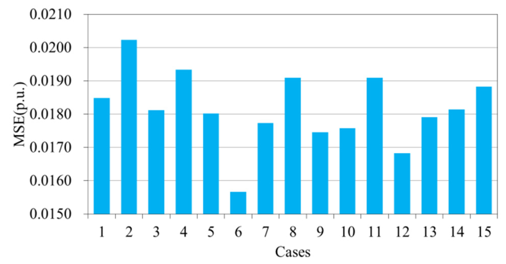
4.3. The Effect of the Order on Performance

In order to analyze the influence of the sub-models’ orders on the performance of the proposed method, 15 cases with different ranking are set, and each case is repeated 30 times. The mean loss functions (i.e., MSE) of the test set are shown in Table 2 and Figure 8.
The following conclusions can be drawn from Figure 8 and Table 2: (1) Comparing the loss functions of Case 6, Case 13, Case 14, and Case 15, it is found that multiple different sub-models are more conducive to improving the performance of the ensemble model than multiple identical sub-models. (2) Sometimes, the performance of the ensemble model composed of different sub-models may not be better than that of another ensemble model with the same sub-models, because the performance of the former is significantly affected by the order of different sub-models. For example, the loss function of Case 2 is larger than those of Case 13, Case 14, and Case 15. Generally, different sub-models can be selected to form the proposed ensemble model, and their order should be determined by the loss function of the validation set.

4.4. Comparative Analysis with Baselines

Normally, the dynamic reactive power optimization can be simplified into multiple static reactive power optimization problems using the time interval control strategy [12]. Specifically, the power load curve is divided into multiple time intervals, and then the static reactive power optimization is performed in each time interval to obtain a comprehensive dispatching strategy for dynamic reactive power optimization. Therefore, the static reactive power optimization can be used as an example to validate the effectiveness of the proposed method in this section.
To illustrate the effectiveness of the proposed ensemble model, the traditional heuristic algorithm (e.g., GA) and popular data-driven-based algorithms (e.g., CBR, MLP, CNN, and LightGBM) are used as the baselines. Each method is repeated 30 times, and the mean results of the test set are shown in Table 3.
The following conclusions can be drawn from Table 3: (1) Generally, the smaller the power loss and voltage offset, the better the performance of the model. Note that power loss and voltage offset are two conflicting metrics sometimes. Therefore, the comprehensive objective function is presented to balance them to evaluate the model performance in an integrated manner. The larger the comprehensive objective function, the better the performance of the model. Specifically, the average comprehensive objective function of CBR is the smallest, which shows that dispatching strategies of historical cases found by the CBR are not well suited to current cases, since the historical power load may significantly vary from the current power loads. (2) Although the performance of the ensemble model is slightly weaker than GA with regard to the average comprehensive objective function and its variance, the ensemble model outperforms other data-driven-based algorithms (e.g., CNN, CBR, MLP, and LightGBM) due to the fact that the average comprehensive objective function of the ensemble model is larger than those of data-driven-based algorithms. This phenomenon shows that the ensemble model can seek better performance from multiple sub-models for reactive power optimization. (3) The online calculation time is one of the important metrics to evaluate the performance of each model for reactive power optimization. Normally, suitable dispatching strategies should be obtained within 60 s [22], during which real-time power systems obtain the observations and then calculate solutions for all power equipment. For single reactive power optimization of the modified IEEE 69-bus radial distribution network, the online time consumptions of the ensemble model, GA, CNN, MLP, LightGBM, and CBR are 0.23 s, 64.77 s, 0.08 s, 0.06 s, 0.09 s, and 4.37 s, respectively. Although data-driven-based algorithms require some time to pre-train models, their online time consumptions are much lower than traditional heuristic algorithms, such as GA. (4) Further, the online calculation time of GA increases significantly with the size of distribution networks (e.g., the number of nodes and equipment), while the online calculation time of the ensemble model is not sensitive to the size of distribution networks, which shows that proposed model is also suitable for reactive power optimization of large-scale distribution networks. This is one of the advantages of the proposed model, i.e., the online calculation time is very short, and is well suited for the real-time optimization of power systems.

4.5. Reactive Power Optimization with Renewable Energy Sources

In order to achieve carbon neutrality, the integration of renewable energy sources in distribution networks has become more and more popular in recent years. To test the performance of different models for reactive optimization of distribution networks with renewable energy sources, the IEEE 33-bus radial distribution network is again modified, as shown in Figure 9.
In particular, the first PV system is added to Node 24 and the second PV system is added to Node 21. The first wind turbine (WT) is added to Node 25, and the second wind turbine is added to Node 12. Assume that the power factor of a node with a wind turbine or PV system is fixed (power factor is 0.95). The power generation of renewable energy sources originates from the National Renewable Energy Laboratory [23,24]. The time resolution of power generation is also 1 h. To ensure that the penetration of renewable energy sources in distribution networks was between 10% and 50%, the original power generation of renewable energy sources is scaled up appropriately. Each method is repeated 30 times respectively and the mean results of the test set are shown in Table 4.
No matter how the penetration changes, the comprehensive objective function value of the proposed ensemble model is the largest, which shows that the ensemble model has better performance than other data-driven-based algorithms (e.g., CNN, CBR, MLP, and LightGBM) for reactive power optimization of distribution networks with different penetration levels.

5. Conclusions

To improve the accuracy and reduce the calculation time of reactive power optimization, a novel ensemble learning-based model is presented in this paper. Through the simulation analysis on two radial distribution networks, the following conclusions are obtained:
(1)
The accuracy of models trained by k-fold cross-validation is higher than that of hold-out validation. In addition, k should not be too small or too large. Four can be considered as a good starting point for k, and higher values or lower values may be fine for other data sets.
(2)
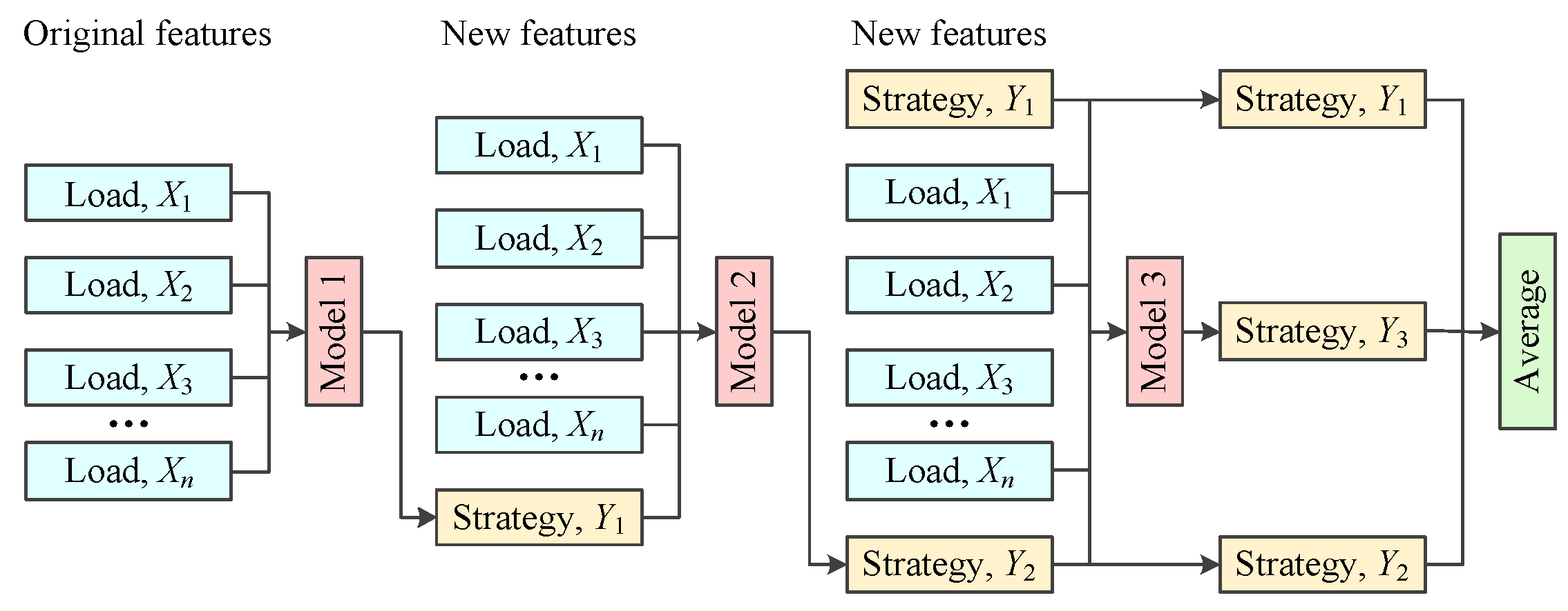
Multiple different sub-models are more conducive to improving the performance of the ensemble model than multiple identical sub-models. Additionally, the performance of the ensemble model is significantly affected by the order of different sub-models. Normally, different sub-models can be selected to form the proposed ensemble model, and their order should be determined by the loss function of the validation set.
(3)
The proposed ensemble model outperforms other data-driven-based algorithms (e.g., CNN, CBR, MLP, and LightGBM) in terms of optimization accuracy and stability. In addition, the calculation time is much lower than the traditional heuristic methods (e.g., GA), especially for large-scale distribution networks.
(4)
No matter how the penetration changes, the ensemble model has better performance than other data-driven-based algorithms (e.g., CNN, CBR, MLP, and LightGBM) for reactive power optimization of distribution networks.

Author Contributions

Data curation, R.Z.; Writing—original draft, R.Z.; Writing—review and editing, B.T. and W.W. All authors have read and agreed to the published version of the manuscript.

Funding

This research was funded by the National Natural Science Foundation of China (No. 52167015) and the Support Project of the Electrical Engineering Laboratory from the Key Laboratory of the Education Department of Tibet Autonomous Region (2021D-ZN-01).

Institutional Review Board Statement

Not applicable.

Informed Consent Statement

Not applicable.

Data Availability Statement

Not applicable.

Conflicts of Interest

The authors declare no conflict of interest.

Nomenclature

Abbreviations
OLTCon-load tap changer
SVCstatic var compensator
PSOparticle swarm optimization
SAsimulated annealing
GAgenetic algorithm
GOSSgradient-based one-side sampling
CBRcase-based reasoning
CNNconvolutional neural network
MLPmulti-layer perceptron
LightGBMlight gradient boosting machine
ReLUrectified linear unit
Adamadaptive moment estimation
Parameters
Wthe weight to balance the power loss and voltage offset
Plossthe power loss before reactive power optimization
P loss the power loss after reactive power optimization
dUthe voltage offset before reactive power optimization
d U the voltage offset after reactive power optimization
nthe number of nodes in distribution networks
Nthe number of branches in distribution networks
U0the rated voltage
Uithe voltage of node i
Rlthe resistance of branch l
Plthe active power of terminal node in the branch l
Qlthe reactive power of terminal node in the branch l
Ulthe voltage of terminal node in the branch l
δ i j the phase difference of the voltage between node i and node j
Gijthe conductance between node i and node j
Bijthe susceptance between node i and node j
Ui,maxthe upper bound of voltage for node i
Ui,minthe lower bound of voltage for node i
Il,maxthe upper bound of current for branch l
nCthe number of nodes with the shunt capacitor bank
nTthe number of nodes with OLTC
nSVCthe number of nodes with SVC
QC,maxthe maximum reactive power generated by the shunt capacitor bank
Ti,minthe minimum tap position of the OLTC
Ti,maxthe maximum tap position of the OLTC
QSVC,maxthe maximum reactive power generated by the SVC
F2a new form of the comprehensive objective function
λ 2 , λ 1 the penalty coefficients
ε the step function
Yconthe output data of convolutional layers
Xconthe input data of convolutional layers
σ con ( ) the activation function of convolutional layers
Wconweights of convolutional layers
Bconbias vectors of convolutional layers
Ypoolthe output data of maximum pooling layers
Xpoolthe input data of maximum pooling layers
Rthe domain of definition for maximum pooling layers
Ydensethe output data of dense layers
Xdensethe input data of dense layers
σ dense ( ) the activation function of dense layers
Wdenseweights of dense layers
Bdensebias vectors of dense layers
Yenthe output data of the encoder
Xenthe input data of the encoder
σ en ( ) the activation function of the encoder
Wenweights of the encoder
Benbias vectors of the encoder
Ydethe output data of the decoder
Xdethe input data of the decoder
σ de ( ) the activation function of the decoder
Wdeweights of the decoder
Bdebias vectors of the decoder
ntrthe number of decision trees
nsathe number of samples
y i ( t ) the forecasting values of the ith sample at the tth iteration
f t ( ) the learned function of the tth decision tree
Ω ( ) a regularization
D ( ) the distance between current forecasts and real values

References

  1. Hui, Q.; Teng, Y.; Zuo, H.; Chen, Z. Reactive power multi-objective optimization for multi-terminal AC/DC interconnected power systems under wind power fluctuation. CSEE J. Power Energy Syst. 2020, 6, 630–637. [Google Scholar] [CrossRef]
  2. Zhao, Q.; Liao, S.; Pillai, J.R. Robust Voltage Control Considering Uncertainties of Renewable Energies and Loads via Improved Generative Adversarial Network. J. Mod. Power Syst. Clean Energy 2020, 8, 1104–1114. [Google Scholar] [CrossRef]
  3. Grudinin, N. Reactive power optimization using successive quadratic programming method. IEEE Trans. Power Syst. 1998, 13, 1219–1225. [Google Scholar] [CrossRef]
  4. Shaheen, A.M.; Spea, S.R.; Farrag, S.M.; Abido, M.A. A review of meta-heuristic algorithms for reactive power planning problem. Ain. Shams. Eng. J. 2018, 9, 215–231. [Google Scholar] [CrossRef] [Green Version]
  5. Liao, W.; Wang, S.; Liu, Q.; Shu, X. Reactive Power Optimization of Distribution Network Based on Case-Based Reasoning. In Proceedings of the 2018 IEEE Power & Energy Society General Meeting, Portland, OR, USA, 5–10 August 2018. [Google Scholar]
  6. Yang, Q.; Wang, G.; Sadeghi, A.; Giannakis, G.B.; Sun, J. Two-Timescale Voltage Control in Distribution Grids Using Deep Reinforcement Learning. IEEE Trans. Smart Grid. 2020, 11, 2313–2323. [Google Scholar] [CrossRef] [Green Version]
  7. Ding, T.; Yang, Q.; Yang, Y.; Li, C.; Bie, Z.; Blaabjerg, F. A Data-Driven Stochastic Reactive Power Optimization Considering Uncertainties in Active Distribution Networks and Decomposition Method. IEEE Trans. Smart Grid. 2018, 9, 4994–5004. [Google Scholar] [CrossRef] [Green Version]
  8. Krannichfeldt, L.V.; Wang, Y.; Hug, G. Online Ensemble Learning for Load Forecasting. IEEE Trans. Power Syst. 2021, 36, 545–548. [Google Scholar] [CrossRef]
  9. Hu, R.; Li, Q.; Lei, S. Ensemble Learning based Linear Power Flow. In Proceedings of the 2020 IEEE Power & Energy Society General Meeting, Montreal, QC, Canada, 2–6 August 2020. [Google Scholar]
  10. Hug, R.; Li, Q.; Qiu, F. Ensemble Learning Based Convex Approximation of Three-Phase Power Flow. IEEE Trans. Power Syst. 2021, 36, 4042–4051. [Google Scholar] [CrossRef]
  11. Lin, R.; Ye, Z.; Wu, B. The application of hydrogen and photovoltaic for reactive power optimization. Int. J. Hydrog. Energy 2020, 45, 10280–10291. [Google Scholar] [CrossRef]
  12. Hu, Z.; Wang, X. Time-interval based control strategy of reactive power optimization in distribution networks. Autom. Electr. Power Syst. 2002, 26, 45–49. [Google Scholar] [CrossRef]
  13. Zhu, R.; Guo, W.; Gong, X. Short-Term Photovoltaic Power Output Prediction Based on k-Fold Cross-Validation and an Ensemble Model. Energies 2019, 12, 1220. [Google Scholar] [CrossRef] [Green Version]
  14. Wong, T.; Yeh, P. Reliable Accuracy Estimates from k-Fold Cross Validation. IEEE Trans. Knowl. Data Eng. 2020, 32, 1586–1594. [Google Scholar] [CrossRef]
  15. Sarhan, M.H.; Nasseri, M.A.; Zapp, D.; Maier, M.; Lohmann, C.P.; Navab, N.; Eslami, A. Machine Learning Techniques for Ophthalmic Data Processing: A Review. IEEE J. Biomed. Health Inform. 2020, 24, 3338–3350. [Google Scholar] [CrossRef] [PubMed]
  16. Aslam, N.; Ramay, W.Y.; Xia, K.; Sarwar, N. Convolutional Neural Network Based Classification of App Reviews. IEEE Access 2020, 8, 185619–185628. [Google Scholar] [CrossRef]
  17. Chen, T.; Xun, J.; Ying, H.; Chen, X.; Feng, R.; Fang, X.; Gao, H.; Wu, J. Prediction of Extubation Failure for Intensive Care Unit Patients Using Light Gradient Boosting Machine. IEEE Access 2019, 7, 150960–150968. [Google Scholar] [CrossRef]
  18. Baran, M.E.; Wu, F.F. Network reconfiguration in distribution systems for loss reduction and load balancing. IEEE Trans. Power Del. 1989, 4, 1401–1407. [Google Scholar] [CrossRef]
  19. Baran, M.; Wu, F.F. Optimal sizing of capacitors placed on a radial distribution system. IEEE Trans. Power Del. 1989, 4, 735–743. [Google Scholar] [CrossRef]
  20. Low Carbon London Project. Available online: https://data.london.gov.uk/dataset/smartmeter-energyuse-data-in-london-households (accessed on 20 February 2022).
  21. Liao, W.; Yang, D.; Wang, Y.; Ren, X. Fault diagnosis of power transformers using graph convolutional network. CSEE J. Power Energy Syst. 2021, 7, 241–249. [Google Scholar] [CrossRef]
  22. Voltage Control in the Future Power Transmission Systems. Available online: https://vbn.aau.dk/ws/portalfiles/portal/254173904/ (accessed on 20 February 2022).
  23. Draxl, C.; Clifton, A.; Hodge, B.; McCaa, J. The Wind Integration National Dataset (WIND) Toolkit. Appl. Energy 2015, 151, 355–366. [Google Scholar] [CrossRef] [Green Version]
  24. Solar Integration National Dataset Toolkit. Available online: https://www.nrel.gov/grid/sind-toolkit.html (accessed on 3 March 2022).
Figure 1. The framework of the proposed method.
Energies 15 01966 g001
Figure 2. The framework of k-fold cross-validation for reactive power optimization.
Energies 15 01966 g002
Figure 3. A simple structure of CNN.
Energies 15 01966 g003
Figure 4. A simple example of the maximum pooling operation.
Energies 15 01966 g004
Figure 5. A simple example of MLP.
Energies 15 01966 g005
Figure 6. Topology of modified IEEE 33-bus radial distribution network.
Energies 15 01966 g006
Figure 7. Topology of modified IEEE 69-bus radial distribution network.
Energies 15 01966 g007
Figure 8. Results of ensemble models with different orders.
Energies 15 01966 g008
Figure 9. Topology of modified IEEE 33-bus radial distribution network with renewable energy sources.
Energies 15 01966 g009
Table 1. Results of ensemble models with different parameters.
CasesMSE (p.u.)Training Time (s)CasesMSE (p.u.)Training Time (s)
hold-out0.02001414.51k = 80.0164778.76
k = 20.0173 108.53 k = 90.0162 854.20
k = 30.0159 206.67 k = 100.0167 895.95
k = 40.0157 294.97 k = 110.0160 977.53
k = 50.0165 386.76 k = 120.0162 1100.97
k = 60.0167 481.69 k = 130.0170 1209.63
k = 70.0163 635.90 k = 140.0195 1389.93
Table 2. The different cases.
CasesOrder of Sub-ModelsCasesOrder of Sub-Models
Case 1CNN, MLP, LightGBMCase 9MLP, CNN, CNN
Case 2CNN, LightGBM, MLPCase 10MLP, LightGBM, LightGBM
Case 3MLP, CNN, LightGBMCase 11LightGBM, MLP, MLP
Case 4MLP, LightGBM, CNNCase 12LightGBM, CNN, CNN
Case 5LightGBM, CNN, MLPCase 13CNN, CNN, CNN
Case 6LightGBM, MLP, CNNCase 14MLP, MLP, MLP
Case 7CNN, LightGBM, LightGBMCase 15LightGBM, LightGBM, LightGBM
Case 8CNN, MLP, MLP
Table 3. The average results of different methods.
NetworksMethodsPower Loss (MW)Voltage Offset (p.u.)Comprehensive Objective Function (p.u.)Calculation Time (s)
Mean ValueVarianceMean ValueVarianceMean ValueVariance
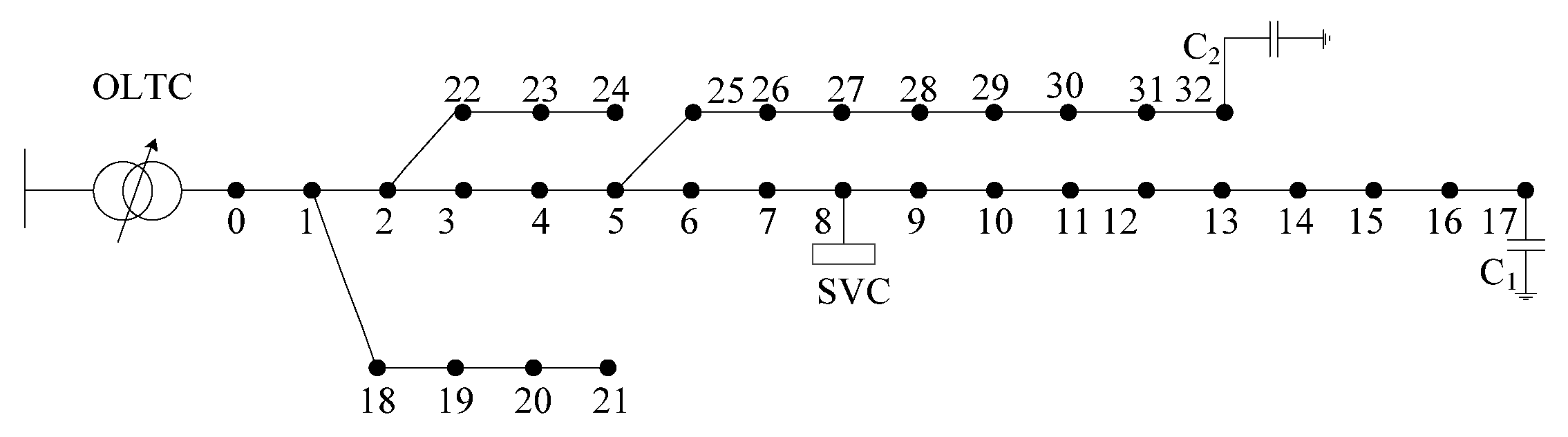
The modified IEEE 33-bus radial distribution networkEnsemble model0.23140.12900.79750.28511.14110.02910.17
GA0.23160.12860.79420.28541.14230.028821.30
CNN0.23160.12920.80280.28581.13960.02920.06
MLP0.23180.12950.81080.28831.13830.02940.04
LightGBM0.23170.12920.80520.28651.13920.02920.07
CBR0.23170.12860.81790.29331.13390.03284.01
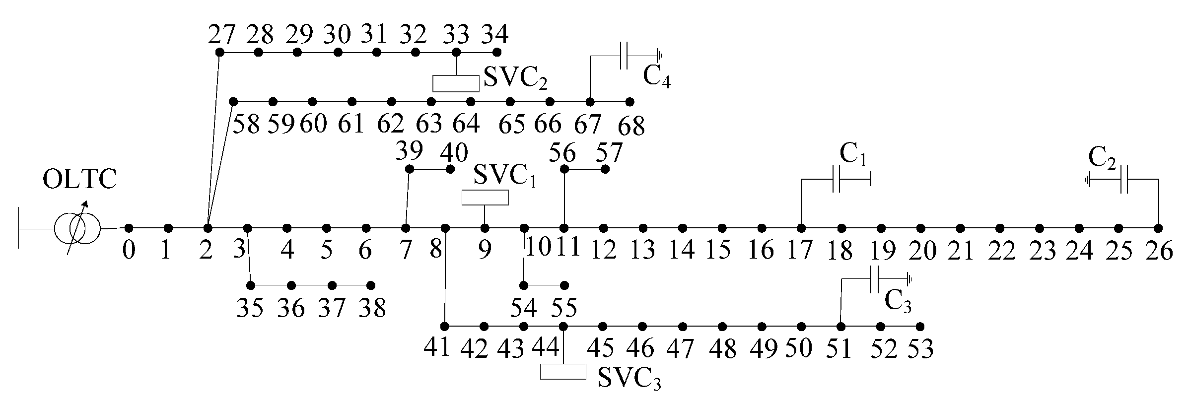
The modified IEEE 69-bus radial distribution networkEnsemble model0.63310.12843.63110.28610.83430.03490.23
GA0.63320.12733.62780.28670.83670.034564.77
CNN0.63370.12873.63640.28730.83290.03520.08
MLP0.63340.12933.64440.29440.83170.03580.06
LightGBM0.63390.1293.63880.29210.83230.03520.09
CBR0.63460.12643.65150.29770.82390.03964.37
Table 4. The average comprehensive objective function for reactive power optimization of distribution networks with renewable energy sources.
Penetration Level (%)Ensemble ModelCNNMLPLightGBMCBR
10%1.13911.12661.12581.12371.1055
20%1.11731.11131.11041.10971.1044
30%1.10951.10631.09881.09751.0953
40%1.09751.09441.09331.099211.087
50%1.07821.06771.06441.06431.064
Publisher’s Note: MDPI stays neutral with regard to jurisdictional claims in published maps and institutional affiliations.

