Optimal Design of C-Type Filter in Harmonics Polluted Distribution Systems

Abstract

This paper aims to find the optimal size of parameters of a C-type filter in a non-sinusoidal system using a new optimization method called the Archimedes optimization algorithm (AOA). The inductance and capacitance values of the filter are acquired in which the power loss in the Thevenin resistor and the power loss characteristics of the load bus are minimized based on a new proposed objective function. Subject to technical and practical limitations of the IEEE 519 standard, an optimization problem is defined to achieve an optimal filter design that can increase the system power quality. The effectiveness of the proposed method is proved by comparison with the recent previously published methods. The results show the effectiveness of the proposed approach using the AOA in finding the minimum power losses and the harmonic content of frequency-dependent components. Eventually, the current study confirmed that the suggested objective function minimizes power losses of fundamental and harmonic order harmonics in non-sinusoidal systems.

1. Introduction

Harmonics and distorted waveforms are one of the main power quality (PQ) problems in the power network since the initial development of the alternating current (AC) system. The growing utilization of power electronic apparatus and nonlinear loads aggravate the PQ. Nowadays, advancement in power networks causes the new challenges in the PQ which can be referred to as the integration of large-scale renewable energy-based generation technologies, and the interconnected power grids growth. These nonlinear loads generate currents and voltages with frequencies higher than the main frequency, which are named harmonic. Paying attention to PQ issues such as harmonics are imperative for power system reliable performance [1,2,3,4,5].

Harmonic pollutions are generated by modern electronic and power electronic loads that can be seen in all industrial devices. By increasing the number of nonlinear loads in distribution systems, the load power factor (PF) decreases, losses increase, and system efficiency reduces, due to the fact that nonlinear loads are categorized as the harmonic current and harmonic voltage sources. When the harmonic distortion goes beyond the standard levels, it causes numerous issues such as poor energy efficiency, excessive power loss, and overheating problems due to harmonic overloading of frequency-dependent apparatuses including lines, transformers, cables, and motors. This issue can reduce their load capacity, protection equipment malfunction, revenue measurement errors, and possibility of resonances at various harmonic frequencies that leads to voltages and currents spikes [6,7,8,9,10,11,12,13,14,15,16,17].

There are several harmonic mitigation methods for reduction or elimination of the impact of the harmonic, including a K-factor transformer [18], a tuned harmonic filter [19], an active filter [20], and a shifting transformer [21]. Among the various techniques and power conditioning strategies that increase the PQ and diminish harmonics, passive filters are broadly used for the maintenance of voltage, economic performance in reactive power compensation, and harmonic modification in power networks, for they have low cost, simplicity, easy monitoring and maintenance, and good reliability [22].

Active power filters (APFs) have been used for reactive power and harmonic compensations. The injection of a compensating current is the principle of operation for active power filters where the injected current has equal magnitude and opposite sign in order to cancel the harmonics and consequently regulate voltage. An active power filter is a group of power electronics-based filters that will utilize components like an amplifier for its functioning. APFs are effective for small nonlinear loads, but are not feasible and cost-effective for large rated nonlinear loads. Their installation and running costs are high since they require high performance voltage (or current) source converters. The initial and operational costs are relatively high due to its high dc-link operating voltage during inductive loading. In addition, it needs a complex control system, and therefore it is only suitable for low or moderate frequencies and cannot handle a large amount of power [23,24].

However, passive power filters were broadly implemented to suppress harmonic current and compensate reactive power in distribution power systems due to their low-cost, simplicity, and high-efficiency characteristics. They can handle large voltage, current and power without power supply requirement. They do not need the additional dc power supply for their operation. However, regardless of numerous advantages, passive filters are not very effective in some conditions including transients, presence of higher order harmonics, and resonance issues [25,26].

To improve the limitations of conventional shunt passive filters, a quasi-passive filter (QPF) has been proposed which comprises of a parallel and series tuned LC circuit. With some variations, the QPF can be used [25]. Inverters have been used to connect distributed generation systems to grids and it is very important to achieve high quality waveforms with the least possible switching transitions number. The well-known selective harmonic elimination pulse width modulation (SHEPWM) method can remove some definite harmonics. Reference [26] suggests an optimal selective harmonic mitigation method that allocates the necessary number of switching angles between different multilevel inverter voltages levels. Consequently, switching frequency has been reduced to the least possible amount. In addition, a special technique is also used to reduce the individual harmonics as much as possible. In [27], the designed coupling LC is based on the reactive power consumption, whereas the planned dc-link voltage level is based on the maximum reactive power compensation range of the LC-HAPF (harmonic active passive filter). Hence, even if the reactive power compensating range was insignificant with a low dc-link voltage, the LC-HAPF could provide dynamic reactive power compensation. Consequently, the reactive power compensation capability is still effective.

Among the various types of passive filters, high-pass passive filters are customary, especially for heavy industrial and HVDC applications, besides transmission systems due to resonance damping of harmonic, voltage support, the loss reduction, and harmonics mitigation. When harmonic pollution is not identified or is hard to forecast, these filters are widely used. Based on their connection, passive filters are categorized into the series and shunt filters. Series type of passive filters creates a high-impedance series path which leads to block harmonics at the tuning frequency, whereas shunt filters present a low-impedance shunt path and consequently harmonics are diverted at the tuning frequency. To mitigate harmonics, shunt filters were implemented more than series filters because series filters have more fundamental harmonic power loss and voltage drop. Shunt filters were categorized, based on their function, into tuned and damped filters. Tuned filters are filters which are designed to reduce harmonics by creating a low impedance path at one, two, or even three tuning harmonic frequencies. Single-tuned filters are usually implemented in distribution systems and industrial applications, whereas the double-tuned and the triple-tuned filters are used in high-voltage applications and HVDC systems. Damped filters are used to filter a wide range of frequencies. The most common damped filters are the second-order, third-order, and C-type filters [28,29].

From the viewpoint of optimization methods for filter designing, research works in literature can be categorized into several classes, which include classical linear and nonlinear approaches [30], sequential quadratic programming [31], and metaheuristic methods. Various metaheuristic approaches for optimal filter design were represented using adaptive carrier frequency optimization [10], non-dominant genetic algorithm (NSGA-II) [32], bee colony [33], adaptive bacterial nutrition optimization [34], differential evolution [35], the cuckoo search algorithm [36], the crow search algorithm [37], the bat algorithm [38], and the Harris Hawks optimization algorithm (HHO) [29]. Generally, the complex problems can found by metaheuristic methods that offer solutions in accordance to constraints and non-constraints. Next, the global behavior has been improved by organizing the interaction between exploration and exploitation to create a robust search path that can escape local optima and achieve global or near-global solutions.

From the solution approach viewpoint, various techniques were proposed to find solutions, such as minimizing harmonic pollution, cost, or power loss, or power factor maximizing, or efficiency [29,30,31,32,33,34,35,36,37,38,39]. A comprehensive overview of the different objective functions (OFs) and constraints for passive filters design was introduced in [40,41,42]. In these references, the harmonic power losses minimization of frequency-dependent components such as transmission lines [40] and cables [41] or transformers [42] were considered.

Compromise about the frequency-dependent weights of harmonic voltage and current vectors was achieved in [29]. In [29], an approach was proposed to design a C-type filter (CTF) to reduce harmonic overloading. It should be noted that the resistances were considered as frequency dependent. For this purpose, a newly developed index is proposed to evaluate the PQ performance of the system with various frequency-dependent components. Non-sinusoidal conditions are indicated by the distortion of the utility voltage and the current distortion of the load.

The proposed objective function (POF) in [29] is developed to minimize cable harmonic losses. However, to achieve this aim, the harmonic losses of the CTF have not been minimized. To address this problem, in this paper, a method for optimal development of a C-type harmonic filter was proposed to adjust harmonic losses of filter and distorted power distribution systems. Besides the harmonic characteristic of source, equipment (cables and transformers) and loads, where all these conditions are instantaneously formulated in an optimization problem, are considered for the optimal design of the CTF. The problem is defined in such a way that its solutions comply with the harmonic constraints reported in the IEEE Standard 519. This problem was solved using a new optimization algorithm called the Archimedes optimization algorithm (AOA), which is based on the physics law known as the principle of the Archimedes. AOA is an intelligent optimizer with fast convergence speed and balance of exploration and exploitation to solve complicated engineering issues [41]. The obtained results by the AOA were compared to the acquired results by HHO for solution validation. The simulation consequences demonstrate well the convergence ability and the efficiency of the represented algorithm for the problem solving of CTF optimum design that is implemented in distribution systems. In addition, the filter designed by the proposed method was confirmed by the efficiency of the POF performance in minimization of the systems power losses in fundamental and harmonic orders components. Generally, in this paper, a new OF is proposed for the optimal design of a CTF. Both harmonic losses of the filter and the harmonic losses of the power system were considered in OF, and the filter design was adapted to moderate these two losses. An optimum design algorithm was primarily established to design a resonance-free CTF. Effective employment of the latest metaheuristic optimization algorithm, the AOA, has been done for the passive harmonic CTF design procedure. In addition, a comparative analysis was done between performances of the third-order high-pass filter and CTF. According to the presented results, the C-type filter leads to the higher PF, system efficiency improvement, and also less transmission loss.

The rest of the paper is organized into five sections. In Section 2, the CTF is represented and formulized. The system under study and the optimization algorithm are proposed in Section 3. Further, performance indices that evaluate the PQ of the system are represented. Section 4 presents the problem formulation and the obtained results are discussed. Finally, the conclusions are represented in Section 5.

2. C-Type Filter: Overview and Design Formulas

The system-independent design was originally introduced in [39] to propose a detuned CTF resonance-free. The word “resonance-free” means that the harmonic voltage magnification produced by the shunt equipment is defined not to be higher than a certain designed threshold, for any system situation. The single-phase equivalent circuit of the CTF is represented in Figure 1. The CTF performs similar to a capacitor ($C_F{}_1$) at the fundamental frequency, causing essentially insignificant and theoretically zero power loss at the fundamental harmonic. The hth harmonic equivalent impedance of the filter can be represented as (1):

$$Z_F^h=R_F^h+j{X}_F^h$$

(1)

$$R_F^h=\frac{R{({\omega }^2{L}_F{C}_F{}_2-1)}^2}{{\omega }^2{(R{C}_{F2})}^2+{({\omega }^2{L}_F{C}_{F2}-1)}^2}$$

(2)

$$X_F^h=\frac{(R^2{C}_{F2}^2{L}_F{C}_{F1}-L_F{}^2{C}_{F2}^2){\omega }^4+(2L_F{C}_{F2}-R^2{C}_F{}_2{C}_{F1}-R^2{C}_{F2}^2){\omega }^2-1}{\omega C_{F1}({\omega }^2{(R{C}_{F2})}^2+{({\omega }^2{L}_F{C}_{F2}-1)}^2)}$$

(3)

where the harmonic equivalent impedance is $Z_F^h$, $R_F^h$ is the filter equivalent resistor, and $X_F^h$ is its reactance.

According to [38], the scheme situations for a CTF are represented in Figure 2 and investigation of these situations will be explained as follows:

Reactive power support is the first situation. The reactive power output of the filter must be equal to the required amount $Q_{cF}$. This situation defines Equation (4) for showing the relationship between the reactive power and the main capacitor $C_{F1}$.

$$C_{F1}=\frac{Q_c{}_F}{{\omega }_1{V}_r^2}$$

(4)

$$Q_{cF}={\omega }_1{C}_{F1}{V}_r^2$$

(5)

where ${\omega }_1$ is the fundamental angular frequency and $V_r$ is the nominal voltage.

The second situation is the power loss minimization at the fundamental frequency. In this state, $L_F$ and $C_{F2}$ resonate to remove the loss of the fundamental order harmonic that causes:

$$L_F=\frac{1}{{\omega }_1^2{C}_{F2}}$$

(6)

$${\omega }_1=\sqrt{\raisebox{1ex}{$1$}\!\left/ \!\raisebox{-1ex}{$L_F{C}_{F2}$}\right.}$$

(7)

A resonance-free situation process is the third situation. When the device is attached to the system, the harmonic voltage at the connection point varies from $V_{pre}(\omega )$ to $V_{post}(\omega )$. The harmonic voltage amplification ratio ($HVA$) thus can be calculated as (8) [28,29], where $Z_s^h$ is the system impedance, and $R_s^h$ and $X_s^h$ are the real and imaginary components of $Z_s^h$, correspondingly.

$$HVA= \left|\frac{V_{post}(\omega )}{V_{pre}(\omega )}\right| = \left|\frac{Z_F^h}{Z_F^h+Z_s^h}\right| = \left|\frac{R_F^h+j{X}_F^h}{R_F^h+j{X}_F^h+R_s^h+j{X}_s^h}\right|$$

(8)

For a specified frequency, the highest $V_{pre}(\omega )$ take places when the system impedance is only reactive and is identical to the negative of shunt device’s equivalent reactance, which is:

$$R_s^h=0\hspace{1em}\hspace{1em}{X}_F^h=-X_s^h$$

(9)

Under this situation, the largest amount of HVA is:

$$HV{A}_{worst}=\sqrt{1+{(\frac{R_F^h}{X_F^h})}^2}$$

(10)

A resonance-free state can be definite as:

$$HV{A}_{worst}\le HV{A}_{limit}\hspace{1em}\hspace{1em}forʠh\ge h_t$$

(11)

where $HV{A}_{limit}$ is a user-identified parameter and $h_t$ is the tuning frequency.

At various frequencies, the system impedance is usually inductive rather than capacitive. Inductive impedance condition is the latest design situation. In this situation, the CTF must show inductive impedance beyond its tuning frequencies, which is:

$$X_F\ge 0\hspace{1em}\hspace{1em}for h\ge h_t$$

(12)

3. Analysis of the System under Study

3.1. System under Study

In this paper, the optimal design of a passive CTF for a conventional industrial power system is studied. To acquire the current, voltage, and power for the studied system, its single-phase equivalent circuit is represented in Figure 3. The load bus includes a three-phase linear load, nonlinear load, individual capacitor, and CTF. A power cable that transmits energy from the transformer to the loads and a CTF connected to the load bus [41,42,43]. It should be noted that, in this paper, two scenarios are investigated. In the first scenario, some linear loads are compensated by an individual capacitor; in the second scenario, no individual capacitor is used for connected loads.

As shown in Figure 3, a linear impedance ($Z_L^h=r_L^h+j{x}_L^h$) and a constant current source per harmonic represent the linear and nonlinear load model parameters, where h is the harmonic order. The denoted hth harmonic impedance of the individual compensation capacitor, which is pre-installed for the linear loads on the customer side, is represented by $Z_{cc}^h=-j{x}_{cc}^h$. The utility side can be modeled by a Thevenin equivalent voltage source and a Thevenin equivalent impedance $Z_s^h=r_s^h+j{x}_s^h$ for each harmonic order. The hth harmonic resistance of the voltage source can be expressed as:

$$r_s^h=r_s^1(1+\frac{0.646h^2}{192+0.518h^2})$$

(13)

where R_S is the fundamental harmonic resistance of the voltage source. Additionally, the hth harmonic inductive impedance of the cable can be written as:

$$Z_c^h=r_c^h+j{x}_c^h$$

(14)

$$r_c^h=r_c^1(0.187+0.532\sqrt{h})$$

(15)

$$x_c^h=h{x}_c^1$$

(16)

The consumer transformer can be essentially modeled by its primary referred harmonic short circuit impedance to its primary side [41,42,43,44].

$$Z_t^h=r_t^h+j{x}_t^h$$

(17)

$$x_t^h=h{x}_t^1$$

(18)

$$S_{max,Tr}(pu)=3V_{(pu)}{\mathrm{I}}_{max-Tr}$$

(19)

where $x_t^h$ is the transformer inductive reactance at harmonic components and it is signified as $h{x}_t^1$. In addition, $r_t^h$ is the transformer equivalent resistance at harmonic frequency. It consists of one frequency-independent resistance and also two frequency-dependent resistors, namely dc resistance ($r_{dc}$), the resistance of winding stray loss ($r_{st}$), and ($r_{ost}$) resistance associated with the additional stray losses in the transformer tank and its clamps.

$$r_t^h=r_{dc}+h^2{r}_{st}+h^{0.8}{r}_{ost}$$

(20)

According to [45,46], the total three-phase harmonic loading losses of a transformer supplying nonlinear loads are considered as:

$$\Delta p_t=\Delta p_{dc}+\Delta p_{st}+\Delta p_{ost}=3{\displaystyle \sum _{h=1}^h(I_s^h}{)}^2{r}_t^h$$

(21)

3.2. Introducing Performance Indices

To compute performance indices, the line current, as well as PCC and load voltages, must be calculated. The line current and voltages are expressed as follows:

$$I_S^h=\frac{V_S^h+(I_L^h\times Z_{FF}^h)}{Z_S^h+Z_c^h+Z_t^h+Z_{FF}^h}$$

(22)

$$Z_{FF}^h=\frac{1}{\frac{1}{Z_F}+\frac{1}{Z_{{}_l}}+\frac{1}{Z_{cc}}}$$

(23)

$$V_{{}_{PCC}}^h=V_S^h-I_S^h{Z}_S^h$$

(24)

$$V_L^h=V_S^h-I_S^h(Z_S^h+Z_c^h+Z_t^h)$$

(25)

In Equation (22), $I_S^h$ shows the line current complex phasor. Moreover, the load-side voltage and the PCC complex voltages were represented as $V_{{}_L}^h$ in Equation (24) and $V_{{}_{PCC}}^h$ in Equation (25).

By considering the fundamental active power ($P_1$) and apparent power ($S_1$) at the load bus, the true power factor (TPF) and displacement power factor (DPF) can be formulated as follows:

$$P_1=V_L^1{I}_L^1\cos ({\phi }_1), S_1=V_L^1{I}_L^1$$

(26)

$$DPF(\%)=100\times \frac{P_1}{S_1}$$

(27)

$$TPF(\%)=100\times \frac{{\displaystyle \sum _{h=1}^H{V}_L^h{I}_S^h\cos ({\phi }_h)}}{\sqrt{{\displaystyle \sum _{h=1}^H{(V_L^1)}^2}}\sqrt{{\displaystyle \sum _{h=1}^H{(I_S^1)}^2}}}$$

(28)

$$THD{V}_{PCC}=100\times \frac{\sqrt{{\displaystyle \sum _{h=2}^H{(V_{PCC}^h)}^2}}}{V_{PCC}^1}$$

(29)

The total harmonic distortion (THD) of voltage and total demand distortion (TDD) of line-to-line current are expressed as Equations (29) and (30).

$$TDD=100\times \frac{\sqrt{{\displaystyle \sum _{h=2}^H{(I_S^h)}^2}}}{{\mathrm{I}}_{md}}$$

(30)

In addition, the apparent power ($S_E$) and power factor ($P{F}_{HA}$) expressions that compute the non-sinusoidal losses can be represented as follows:

$$S_E=3\sqrt{{\displaystyle \sum _{h=1}^h(V_L^h}{)}^2{C}_v^h}\hspace{0.17em}\sqrt{{\displaystyle \sum _{h=1}^h(I_S^h}{)}^2{C}_i^h}$$

(31)

$$P{F}_{HA}=\frac{{\displaystyle {\sum }_h{V}_L^h}{I}_S^h\cos {\phi }_h}{S_E}$$

(32)

where $C_v^h$ and $C_i^h$ are the hth harmonic weighting factors for voltage and current, respectively. Both are identical at the fundamental frequency (equal to 1). ${\phi }_h$ is the hth harmonic phase angle between the hth line current and load voltage. Different values were considered for $C_v^h$ and $C_i^h$ at harmonic frequencies, but the most suitable values were obtained when setting $C_v^h$ equal to 1 and $C_i^h$ equal to h^1.333, as implied in IEEE 519 limits. It should be mentioned that maximizing $P{F}_{HA}$ leads to the harmonic losses to become minimized.

Another index which should be calculated is loss-based power factor ($P{F}_L$). Maximizing $P{F}_L$ would minimize the components harmonic losses. Under non-sinusoidal conditions, the $P{F}_L$ is stated as:

$$P{F}_L=\sqrt{\frac{\Delta p_{min}}{\Delta p}}$$

(33)

Consequently, for the systems that are distorted by harmonics, the entire power loss ($\Delta p$) can be calculated as:

$$\Delta p=\Delta p_S+\Delta p_t+\Delta p_c$$

(34)

where $\Delta p_{min}$ is achieved by the time I_min, which is when a sinusoidal active current is passing through the system. It can be computed based on the fundamental frequency component of the load voltage, and also the amplitudes of the active power as follows:

$$I=\frac{p_1}{V_1^2}$$

(35)

The correlation between the voltage harmonics and motor load loss function ($MLL$) is specified as Equation (36).

$$MLL(\%)=100\frac{\sqrt{{\displaystyle {\sum }_{h=1}^H\frac{{\left|V_L^h\right|}^2}{h}}}}{V_L^1}$$

(36)

Transmission efficiency is introduced as an index that is used to assess the system load performance. This parameter is represented as:

$$\eta (\%)=100\times \frac{{\displaystyle \sum _{h=1}^H{V}_L^h{I}_S^h\cos ({\phi }_h)}}{{\displaystyle \sum _{h=1}^H{V}_L^h{I}_S^h\cos ({\phi }_h)}+{\displaystyle \sum _{h=1}^H{I}_S^h{}^2(r_t+r_s+r_c)}}$$

(37)

3.3. Optimization Algorithm: Overview, and Formulations

Nowadays, optimization algorithms based on the metaheuristic techniques are frequently used to solve complicated engineering issues due to their exploration and exploitation capabilities to get better results. In this work, AOA, is used to calculate the CTF parameters, for it has good capability to solve subjects [46]. Archimedes’ principle is based on the object immersion in a fluid. The fluid applies a downward force on the object that is the same as the subject weight. The immersed objects are considered as the population individuals in this algorithm. Similar to the other swarm-based metaheuristic procedures, a search procedure is begun by the AOA based on the object’s initial population. These candidate explanations have random volumes, densities, and accelerations values. After that, each object position is adjusted randomly. After the fitness evaluation, the AOA optimization starts and the iterations will be continued as long as the termination complaint happens. The object density and its volume are updated in every repetition, and the object acceleration is informed according to the collision situation of the neighbor object. The AOA can be represented as a global optimization algorithm which involves exploration and exploitation abilities. Figure 4 shows the AOA, and the steps of the represented AOA are detailed as following:

Initialization of the positions of all objects is shown in Equation (38):

$$O_i=l{b}_i+rand\times (u{b}_i-l{b}_i); i=1,2,\dots ,N$$

(38)

where O_i is the ith object in a population of N objects, and $l{b}_i$ and $u{b}_i$ are the lower and upper bounds of the search-space, respectively.

The initialization of the volume ($vol$), density ($den$), and acceleration ($acc$) for each ith object is according to:

$$\begin{gathered} \begin{array}{l}de{n}_i=rand\\ vo{l}_i=rand\end{array} \\ \hspace{1em}\hspace{1em}\hspace{1em}\hspace{1em}\hspace{1em}\hspace{1em} ac{c}_i=l{b}_i+rand\times (u{b}_i-l{b}_i) \end{gathered}$$

(39)

In this step, primary population evaluation and also object selection based on its fitness value will be conducted (x_best, den_best, vol_best, and acc_best). The density and volume of the ith object for the iteration t + 1 is updated using:

$$vo{l}^{t+1}{}_i=de{n}^t{}_i+rand\times (de{n}_{best}-de{n}^t{}_i)$$

(40)

$$vo{l}^{t+1}{}_i=vo{l}^t{}_i+rand\times (vo{l}_{best}-vo{l}^t{}_i)$$

(41)

where $de{n}_{best}$ is the best object density and $vo{l}_{best}$ is its volume, and $rand$ represents the random number. First, a collision happens among objects and, after a short time, the objects attempt to get the stability condition. This is employed in the AOA with the aid of the transfer operator (TF) parameter. This parameter converts the search from exploration to exploitation and it is defined using Equation (42):

$$TF=exp(\frac{t-t_{max}}{t_{max}})$$

(42)

where $TF$ varies with time until it reaches 1. In this equation, $t$ and $t_{max}$ are iteration and maximum iterations numbers, correspondingly. Additionally, d, which is called the density decreasing factor, helps the AOA in global and local searches. It reduces with time Equation (43):

$$d^{t+1}=exp(\frac{t-t_{max}}{t_{max}})-(\frac{t}{t_{max}})$$

(43)

where $d^{t+1}$ reduces with time, to converge in a previously known promising area. Proper supervision of this index balances exploration to exploitation in the algorithm.

If TF ≤ 0.5, object collision happens, a random material (mr) is chosen and an object’s acceleration for repetition t + 1 is updated as:

$$ac{c}_i^{t+1}=\frac{de{n}_{mr}+vo{l}_{mr}\times ac{c}_{mr}}{de{n}_i^{t+1}\times vo{l}_i^{t+1}}$$

(44)

where $de{n}_i$, $vo{l}_i$, and $ac{c}_i$ are density, volume, and acceleration of ith object. In addition, $ac{c}_{mr}$, $de{n}_{mr}$ and $vo{l}_{mr}$ are the acceleration, density, and volume of random material. It is significant to declare that TF ≤ 0.5 confirms exploration through one third of iterations. Applying a value other than 0.5 will change exploration–exploitation behavior.

No collision takes place between objects for TF > 0.5. An object’s acceleration can be updated for repetition t + 1 using:

$$ac{c}_i^{t+1}=\frac{de{n}_{best}+vo{l}_{best}\times ac{c}_{best}}{de{n}_i^{t+1}\times vo{l}_i^{t+1}}$$

(45)

where $ac{c}_{best}$ is the best object acceleration.

Normalized acceleration was implemented to calculate the percentage of variation, as follows:

$$ac{c}_{i-norm}^{t+1}=u\times \frac{ac{c}_i^{t+1}-min(acc)}{max(acc)-min(acc)}+1$$

(46)

where $u$ and l are the normalization variety and are 0.9 and 0.1, correspondingly. The $ac{c}_{i-norm}^{t+1}$ shows the step percentage of each agent. If the object i has a significant distance from the global optimum, the acceleration amplitude will be great, and the object will be in the exploration stage; or else, the object will be in the exploitation stage. Typically, the acceleration agent has a large value at the beginning and reduces with time. This assists search agents to transfer to the global best result, far from local solutions.

If TF is lower than 0.5, the ith object’s position for next iteration t + 1 is:

$$x_i^{t+1}=x_i^t+C_1\times rand\times ac{c}_{i-norm}^{t+1}\times d\times (x_{rand}-x_i^t)$$

(47)

where $C_1$ is a constant equal to 2. Otherwise, the objects update their positions Equation (48):

$$\begin{array}{l}{x}_i^{t+1}=x_{best}^t+F\times C_2\times rand\times ac{c}_{i-norm}^{t+1}\times d\times (T\times x_{best}-x_i^t)\\ T=C_3\times TF\end{array}$$

(48)

where $C_2$ is a constant and it equals to 6. T is time-dependent and it is related to the transfer operator.

The few number of steps and the function consideration requirement for the optimum solution location are considered as the major advantages of this method. On the other hand, the algorithm only solves the convergence problem.

4. Optimization Problem

In this work, the AOA has been implemented to find the optimal design of CTF, while maintaining the desired performance levels. The diagram of the proposed technique is shown in Figure 5. In this section, the proposed optimal filter design approaches are numerically evaluated for the two scenarios in a studied industrial power system. For scenario 1, the individual capacitor was connected in the studied system; for scenario 2, the capacitor was excluded. The fundamental frequency supply voltage and short-circuit power of two simulated systems are 6350 V (line-to-line) and 800 MVA. The OF, constraints and results are given below.

4.1. Proposed Objective Function

The proposed optimization approach in [29] was the minimization of transmission line power losses to reduce harmonic overloading of the frequency-dependent apparatuses in the system, whereas this optimization function did not minimize filter harmonic losses. The conventional optimization approaches, which were the maximization of $P{F}_L$ and the harmonic adjusted power factor, were proposed in [46], respectively, to reduce components’ harmonic overloading in the system. According to the obtained result in [46], $P{F}_L$ increment causes the load power loss increment. Therefore, optimizing the filter according to these OFs has not led to the proper design of the filter in order to reduce the harmonic losses of the whole system.

Consequently, in this paper, a new OF is proposed to optimum the harmonic losses of the load and transmission system. The purpose of this function is to optimize the CTF parameters in order to balance the harmonic losses (both transmission losses and loads bus losses) of the under-studied system. The proposed OF was shown as (48). As shown in this equation, the POF includes two terms. The first term is related to the transmission line losses, and the load losses are proposed in the second term. Accordingly, the minimization of total loss (including fundamental and harmonic losses) is the major goal in this POF.

$$OF=minimize[\frac{{\displaystyle \sum _h{(I_S^h)}^2(r_t^h+r_c^h+r_s^h)}}{\Delta p_r}+\frac{{\displaystyle \sum _{h=1}^H{V}_L^h{I}_S^h}\cos (\phi )+{\displaystyle \sum _{h=1}^H{(I_S^h)}^2}(r_S^h+r_c^h+r_t^h)}{{\displaystyle \sum _{h=1}^H{V}_L^h{I}_S^h}\cos (\phi )}]$$

(49)

It should be noted that optimization of CTF parameters were done for two scenarios, including the individual capacitor and excluding it.

4.2. Constraints

Six constraints have been applied in this paper. The primary limitation is to certify the harmonic components of the voltage limits compliance with the reported value in IEEE 519 for the point of common coupling and load bus voltages [46]. Figure 6 shows the threshold values according to the IEEE 519, which is used in this problem, where $THD{V}_{max}$ is the maximum acceptable amount by IEEE 519 for $THDV$. $IHD{V}_{PCC}^h$ and $IHD{V}_L^h$ represent the hth different harmonic distortion percentages of the point of common coupling and load-bus voltages, respectively. The hth maximum amount allowable for individual harmonic voltage distortion is named $IHD{V}_{max}^h$.

The second limitation is to ensure that the PCC voltages and loads match the bus voltage range. The third restriction is to guarantee passivity with the individual harmonic current and the total demand distortion restraints represented in IEEE 519 for the distorted system currents. The fourth limitation is to guarantee that the TPF range is in its satisfactory boundaries [46]. The fifth constraint is to warrant limitation with shunt capacitor restrictions proposed in IEEE 18-2012 to certify operation of connected capacitors that it is connected to the non-sinusoidal load bus. Specifically, for every shunt capacitor, the capacitor’s rms voltage, peak voltage, rms current, and reactive power must conform to the proposed parameters that are given per-unit based on their nominal amplitudes [46].

$$\begin{array}{l}{V}_{c,k}(C_{F1},L_F,C_{F2},R)\le 1.1\\ V_{cp,k}(C_{F1},L_F,C_{F2},R)\le 1.2\\ I_{c,k}(C_{F1},L_F,C_{F2},R)\le 1.35\\ Q_{cF,k}(C_{F1},L_F,C_{F2},R)\le 1.35\end{array}$$

(50)

The last limitation is to certify that the connected filter attenuates the harmonic resonance that is originated after the connection. It represents based on the load voltages ratio before and after filter connection in the system and according to the worst item of $HV{A}_{worst}$. In this situation, the series system impedance is completely reactive and matches to the negative equivalent filter reactance [29]. Therefore:

$$HV{A}_{worst}^h(C_{F1},L_F,C_{F2},R)\le HV{A}_{{}_{worst}}^{Threshold},\hspace{1em}HV{A}_{{}_{worst}}^{Threshold}=1.2$$

(51)

4.3. Simulation Results

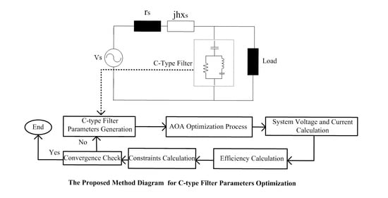
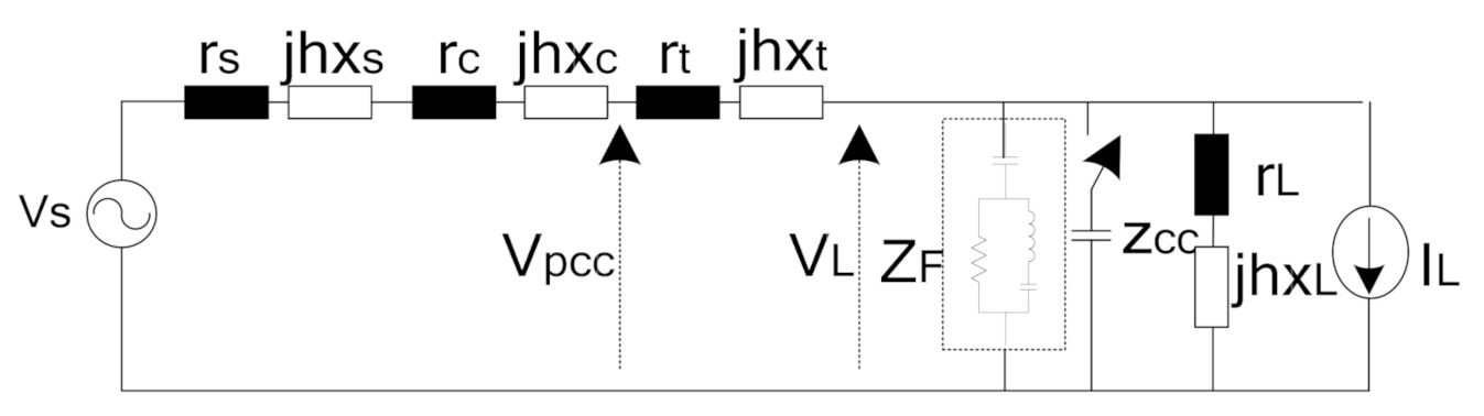
The three-phase short-circuit power of system in Figure 3 is 800 MVA, and the rated line voltage is 6.35 kV. The impedances of the system and load are shown in

Table 1. The load and system characteristics.

Parameter	$r_s^1$	$x_s^1$	$r_t^1$	$x_t^1$	$r_c^1$	$x_c^1$	$r_L^1$	$x_L^1$	$x_{cc}^1$
Value (Ω)	0.0038	0.0506	0.044	0.221	0.0098	0.0104	4	4.05	100

. These values are reported at the fundamental frequency. The equivalent Thevenin resistance is 0.0038 Ω and this value is reported for the first order harmonic component. Its reactance amplitude at this frequency is 0.0506 Ω. A power cable with 640 A ampacity, length of 0.1 km and 6.35 kV rated voltage was considered. It should be noted that its reactance and also resistance values at the fundamental frequency were considered as 0.0098 Ω and 0.0104 Ω. The rated power of the consumer transformer is 7 MVA and its voltage ratio is 6.3 kV/0.4 kV. The transformer resistances are set as 0.026, 0.006, and 0.012 ohms, respectively, and the inductive reactance value is given 0.221 ohms. The load bus powers including active and reactive powers were assumed to be 4.9 MW and 4.965 MVAr. The 4 and 4.05 ohms are the load resistance and reactance, respectively, at the fundamental order harmonic. A capacitor bank compensates the reactive power for the loads, and $x_{cc}^1$ referred to the transformer primary side is 100 Ω.

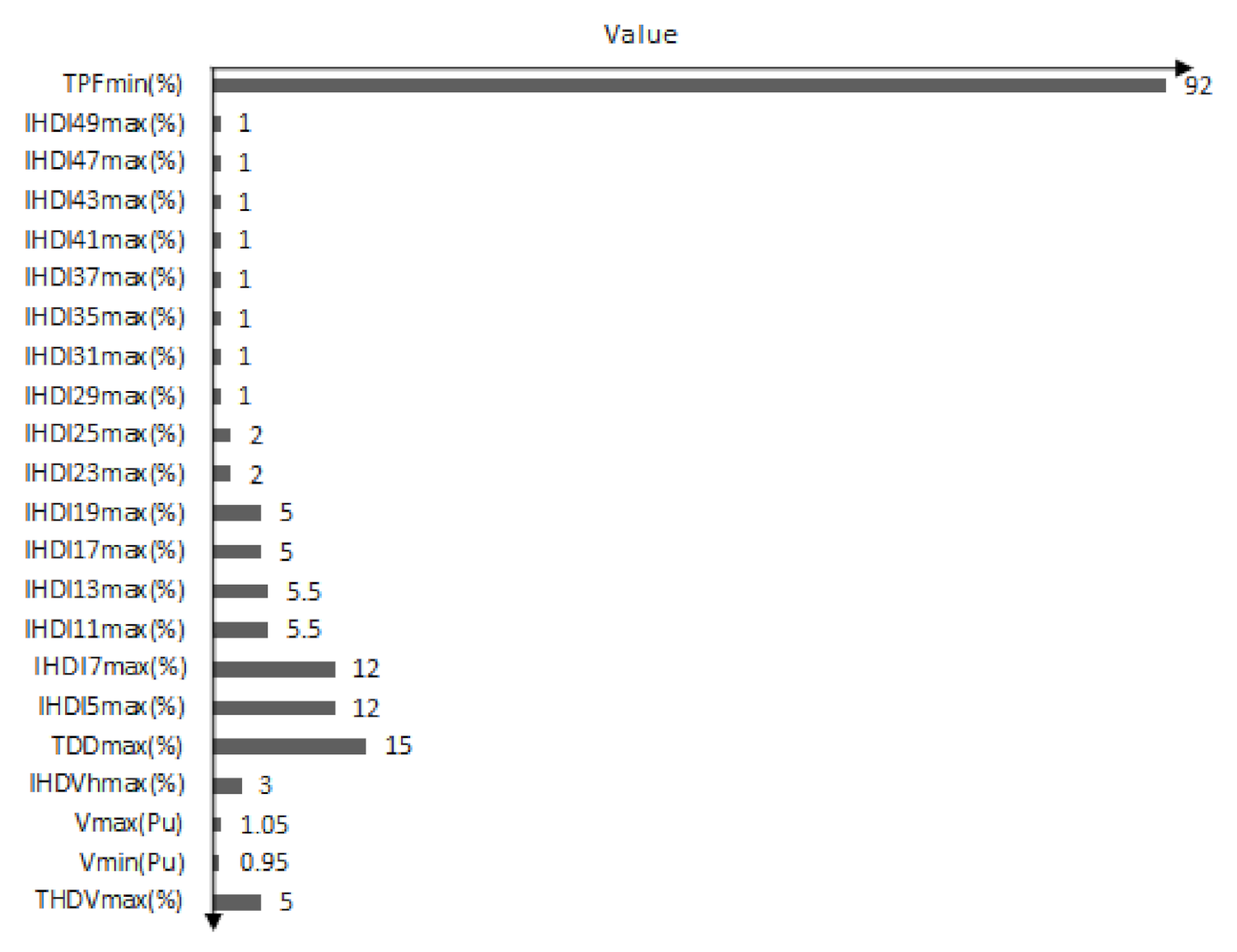
The harmonic characteristic of the system and connected linear load and individual capacitor were calculated based on the proposed Equations (13)–(21) in Section 3. In addition, the nonlinear load was simulated using harmonic current injections at harmonic orders which are shown in

Table 2. The nonlinear loads and utility side’s background harmonic voltage.

Harmonic Order (h)	Nonlinear Load Current (A)	Phase Angle (Degree)	Utility Harmonic Voltage
5	75	$-45\times h$	55
7	65	$-45\times h$	40
11	55	$-45\times h$	35
13	40	$-45\times h$	30
17, 19, 21, 23	15	$-45\times h$	25
29, 31, 35, 37	10	$-45\times h$	12.5
41, 43, 47, 49	7.5	$-45\times h$	7.5

[46]. The harmonic voltage distortion, which is shown in Table 2, is referred to the utility side’s one. The simulations were performed using the MATLAB software package.

The uncompensated system results are tabulated in

Table 3. The uncompensated system results under two scenarios.

Scenario 1
Parameter	Value	Parameter	Value
$I_S(pu)$	0.9596	$P{F}_{HA}(\%)$	45.1853
$V_{PCC}(pu)$	0.9927	$MLL(\%)$	4.4511
$V_L(pu)$	0.9728	$THD{V}_L(\%)$	15.0626
$TPF(\%)$	69.0024	$THD{V}_{PCC}(\%)$	4.1633
$DPF(\%)$	73.1726	$TDD(\%)$	23.7984
$P{F}_L(\%)$	70.2339	$\Delta p(pu)$	1.7519
Scenario 2
Parameter	Value	Parameter	Value
$I_S(pu)$	0.9675	$P{F}_{HA}(\%)$	40.1347
$V_{PCC}(pu)$	0.9854	$MLL(\%)$	5.68
$V_L(pu)$	0.9623	$THD{V}_L(\%)$	17.84
$TPF(\%)$	65.056	$THD{V}_{PCC}(\%)$	5.3741
$DPF(\%)$	70.27	$TDD(\%)$	25.98
$P{F}_L(\%)$	68.27	$\Delta p(pu)$	1.8493

. It can be seen from Table 3 that $THD{V}_{PCC}$ is close to $THD{V}_{max}$, but both $THD{V}_L$ and $TDD$ are significantly greater than their allowable values. It can be concluded from Table 3 that the $THD{V}_{PCC}$ value in scenario 1 is close to the allowable value, $THD{V}_{max}$, (as shown in Figure 6); in scenario 2, due to the lack of individual capacitor, its value has exceeded the allowable limit. However, both $THD{V}_L$ and $TDD$ are significantly higher than their allowable values. In addition, represented results show that the considered power factor expressions, for both scenarios, are very small due to the harmonic pollution and lack of reactive power. The results of scenario 2 also show that the capacitor uninstallation leads to more reduction in total harmonic distortion and power factor, and therefore poorer PQ. It shows that the connected capacitor to the load bus does not affect the DPF value improvement. The motors $MLL$ value also has a high amplitude. In addition, components power losses values are large and it shows that system harmonic overloading aggregated.

As shown in Table 3, the optimum finding of CTF parameters can improve the PQ of the studied system. Therefore, optimization process based on the OF presented in (49) was performed. In addition, to find the optimization problem, the AOA and the HHO algorithms were implemented using the MATLAB software package. The search agents’ number and the maximum iterations number were set to 50 and 400, correspondingly. The presented results are reported as an average value over 30 independent runs.

The optimal parameters for the simulated filter and the best fitness amplitudes by the HHO and the AOA algorithms are given in

Table 4. The optimal filter parameters and the best fitness values.

	AOA	HHO	AOA	HHO
	Scenario 1		Scenario 2
CF1(mF)	0.31189	0.332	0.3765	0.04105
CF2(µF)	94,068	94,218	84,672	96,413
LF(mH)	1.27	1.174	1.41	1.32
R(Ω)	3.2452	3.256	4.254	4.398
Best	5	33	37	7
Mean	6.7	25.3	38.5	7.5
Standard Deviation	0.13	0.136	0.12	0.14
Time(s)	181.32	184.58	182.13	185.97

. Moreover, the worst, mean, and standard deviation of the obtained fitness parameters and the computation times are explained in the same table.

It is shown in Table 4 that the two considered algorithms represent the best fit parameters. For scenario 1, the represented results by the AOA are superior to the results of the HHO optimizer in terms of best-fit (=5) and mean (=6.7) values. The minimum values of the standard deviation index of the AOA (0.13) and the HHO (0.136) indicate their high robustness. In addition, the AOA has a lower time for computation to reach the best fitness value than the HHO algorithm over the identical iterations number, and also the runs. According to the results, it is clear that the capacitors amount used in the CTF in scenario 2 is more than in scenario 1, because in scenario 1, a portion of the reactive power of the load is supplied by the individual capacitor. Therefore, lower reactive power will be delivered from the filter in this plan.

The comparison of the results show that the optimal solution is achieved with better standard deviation and running time. The results also show that the proposed method might have advantages when compared with the proposed method in [29].

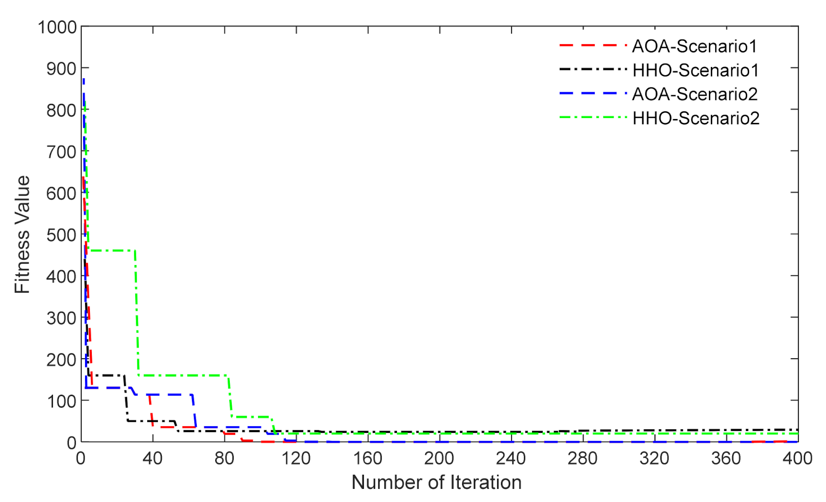
In addition, the convergence rate for both algorithms and both studied scenarios were illustrated in Figure 7 for the sake of a better comparison between the two implemented algorithms. This is a typical diagram for 30 run numbers that, for example, a sample convergence diagram has been shown in Figure 7. The compensated system results and also the optimum calculated parameters for the studied filter for the proposed OFs are tabulated in

Table 5. The optimal filter parameters and results for the compensated system for the two scenarios.

	Scenario 1	Scenario 2
CF1(mF)	0.31189	0.3765
CF2(µF)	94068	96672
LF(mH)	1.27	1.41
R(Ω)	3.2452	4.254
$I_S(pu)$	0.7642	0.7693
$V_{PCC}(pu)$	0.9997	0.9945
$V_L(pu)$	0.9957	0.9854
$TPF(\%)$	98.56	92.13
$DPF(\%)$	99.96	94.34
$P{F}_L(\%)$	92.63	87.49
$P{F}_{HA}(\%)$	91.56	83.23
$MLL(\%)$	1.34	1.69
$THD{V}_L(\%)$	3.17	3.69
$THD{V}_{PCC}(\%)$	3.58	4.17
$TDD(\%)$	8.95	9.95

.

For the uncompensated system, a negligible harmonic current can make very high voltage distortion, as displayed in Table 3, due to the nonlinear relationship between them [28]. Comparison of the results presented in Table 3 and Table 5 shows that the general performance of the proposed method is satisfactory. Table 5 shows that the proposed technique leads to the supply current reduction, lower transmission losses, higher transmission efficiency, and higher loads power factor than the non-compensated system parameters represented in Table 3. In addition, it is clear that the total harmonic voltage distortion is intensely diminished, satisfying the required OF and complying with the IEEE standard 519-1992.

According to the results, CTF implementation increases the PF and the DPF, and decreases the voltage THD, thus avoiding the production of harmonic currents in the network. As presented in Table 5, for the two scenarios of the compensated system, the total harmonic distortion indices (THDV and THDI) measured at the PCC and load bus are below the IEEE standard limit (5%). The TDD values are lower than the IEEE standard constraint (15%) in all achieved results.

It can be seen that the $C_{F1}$ and $C_{F2}$ values provided by scenario 1 have fewer amplitudes than obtained values in scenario 2; therefore, lower reactive power will be passed, even though the filter’s resistor (R) and its inductive property (LF) provided by scenario 1 have lower amplitudes than the obtained results by the scenario 2. In addition, Table 5 shows the filter parameters that have been calculated based on the scenario 1.

According to these calculated parameters, a lower $I_S(pu)$ has been obtained than in the other scenario. Besides, as represented in Table 5, the suggested filter design by scenario 1 results in higher $TPF(\%)$ and $DPF(\%)$ compared to the other scenario. In addition, $MLL(\%)$ is superior to values that have been achieved by scenario 1.

As represented in Table 5, the filter parameters calculated by scenario 1 resulted in lower harmonic distortion values than in scenario 2. This issue clarifies a lower harmonic system component risk.

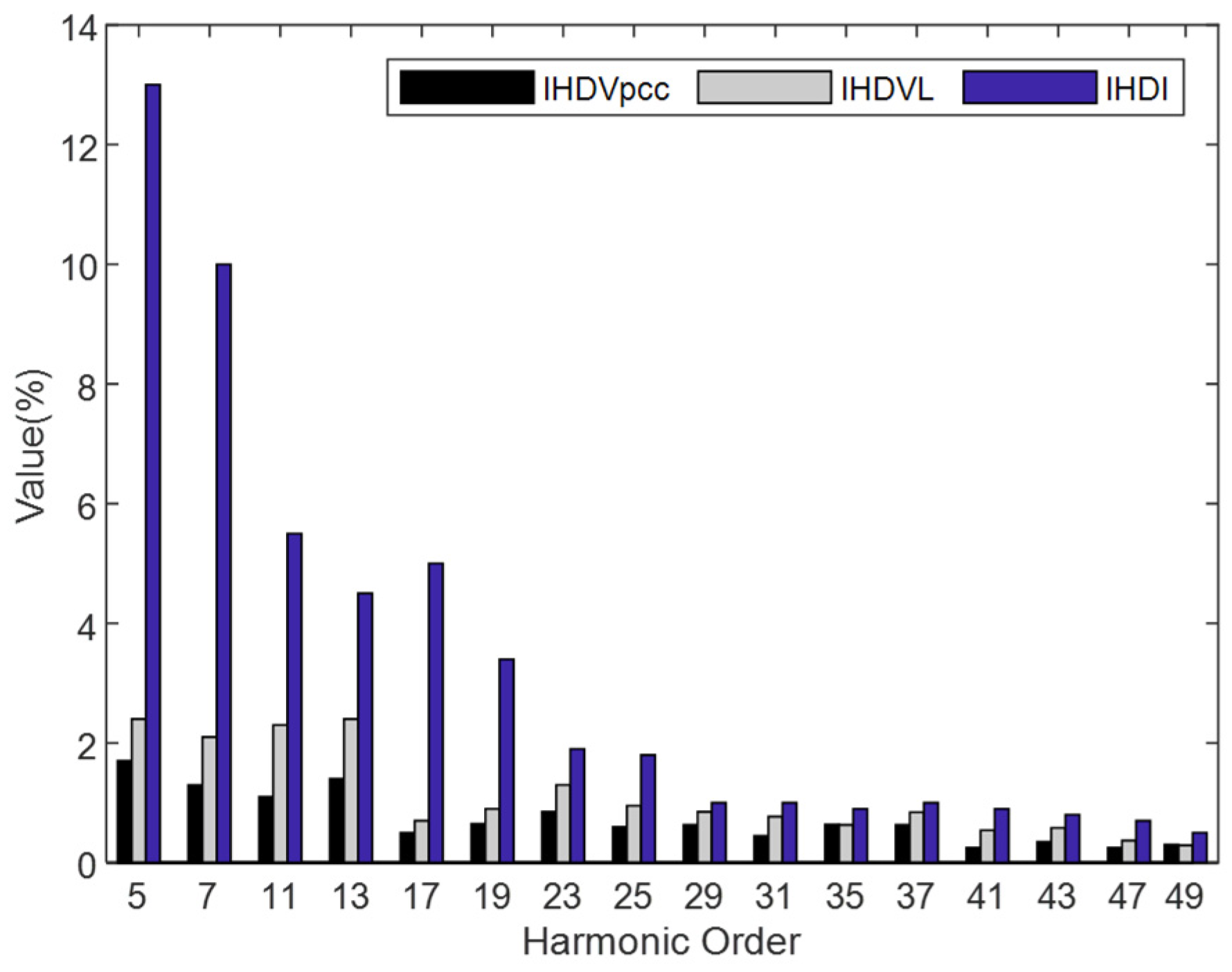
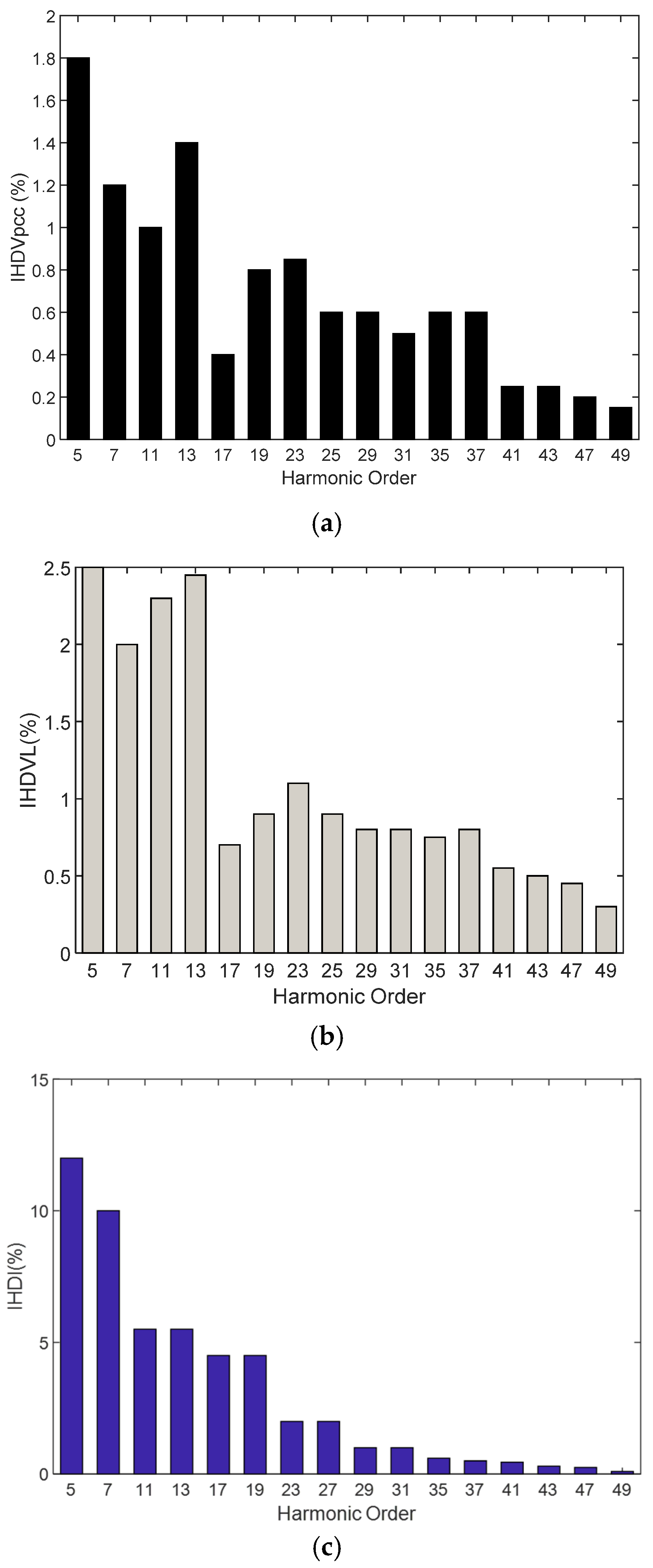
Moreover, the different harmonic amplitudes of current and also voltage, shown in Figure 8 and Figure 9 for $IHD{V}_{PCC}$, $IHD{V}_L$, and $IHDI$, are lower than the IEEE 519 limits for every order of harmonics, which have been presented in Figure 6. As shown in Figure 8 and Figure 9, for both two scenarios, the IHDV and IHDI are below the IEEE standard limit. Moreover, these parameters for scenario 2 have higher values than scenario 1. This condition is due to the fact that some harmonic distortions were compensated by the individual capacitor in scenario 1.

To show the POF performance, the CTF parameters which have been optimized in this paper were compared with the results obtained from the OF in [29]. Both simulations were done for scenario 1 and based on the AOA method. The obtained results are represented in

Table 6. Comparison of the POF and the represented OF in [29], based on the AOA.

	Proposed Objective Function (POF)	Objective Function (OF) in [29]
CF1(mF)	0.31189	0.3243
CF2(µF)	94068	9506
LF(mH)	1.27	1.165
R(Ω)	3.2452	3.3091
$I_S(pu)$	0.7642	0.7732
$V_{PCC}(pu)$	0.9997	0.9989
$V_L(pu)$	0.9957	0.9949
$TPF(\%)$	98.56	97.96
$DPF(\%)$	99.96	98.99
$P{F}_L(\%)$	92.63	91.85
$P{F}_{HA}(\%)$	91.56	90.84
$MLL(\%)$	1.34	1.54
$THD{V}_L(\%)$	3.17	3.56
$THD{V}_{PCC}(\%)$	3.58	3.64
$TDD(\%)$	8.95	9.15
$\eta (\%)$	99.03	99.83

.

It can be noticed that $P{F}_L$ and $P{F}_{HA}$ are improved from 91.85% to 92.63% and 90.84 to 91.56, respectively. $\eta$ is increased from 99.03% to 99.83%. Furthermore, all two methods provide almost all the $TDD$ and $THDV$ values below the standard threshold. For both OFs, the amount of harmonic voltage distortion, as well as the $TDD$, is less than the standard thresholds. In addition, the calculated $I_S$ by the POF has a smaller amplitude than the proposed method in [29]. According to the results, the obtained values of C_F1 and C_F2 in the POF have lower values. This indicates that less reactive power must be injected into the system by the CTF. $TPF(\%)$ and $DPF(\%)$ for the POF have higher amplitudes rather than the function proposed in [29]. Calculated $MLL$ by the POF has been improved compared to the previous works due to the harmonic dependency of these parameters. Generally, the achieved results indicate an effective harmonics reduction in the studied system compared to the OF in [29].

The comparison of the results shows that, based on the POF, the optimal solution is achieved with a better power factor, higher transmission efficiency and lower losses in Thevenin’s resistor. Additionally, the results proved that the proposed method has better performance compared to the proposed method in [29], where all the resultant values of THD are lower than for other investigated cases. Besides, Figure 10 shows the $IHD{V}_{PCC}$, $IHD{V}_L$, and $IHDI$, respectively which were calculated based on the proposed OF in [29] by the AOA algorithm. As shown in Figure 10, the voltage and current distortion values of the individual harmonic are well below the IEEE 519 limits for the individual harmonic distortion limits, but by comparing Figure 8 and Figure 10, it is obvious that the POF leads to the lower individual harmonics amplitudes compared to the proposed OF in [29].

In addition, to validate the proposed method, the obtained simulation results were compared with the results and findings of [29]. All results were reported based on the Harris Hawks algorithm, as tabulated in

Table 7. Comparison of the POF and the represented OF in [29] based on the Harris Hawks algorithm.

	Proposed Objective Function	Objective Function in [29]
CF1(mF)	0.332	0.39863
CF2(µF)	94218	9200
LF(mH)	1.174	1.1
R(Ω)	3.256	3.0754
$I_S(pu)$	0.7003	0.7137
$V_{PCC}(pu)$	0.9995	0.9994
$V_L(pu)$	0.9955	0.9966
$TPF(\%)$	98.55	98.58
$DPF(\%)$	99.86	99.65
$P{F}_L(\%)$	89.95	86.38
$P{F}_{HA}(\%)$	91.23	90.77
$MLL(\%)$	1.42	1.57
$THD{V}_L(\%)$	3.77	4.79
$THD{V}_{PCC}(\%)$	2.56	2.71
$TDD(\%)$	9.04	10.21

. As shown in Table 7, the achieved results based on the proposed objective function in [29] are similar to the obtained results in this reference. In addition, the proposed objective function has better performance compared to the objective function in [29]. It can be noticed that $P{F}_L$ and $P{F}_{HA}$ are improved from 86.38% to 89.95% and 90.77 to 91.23, respectively. Furthermore, all two objective functions provide almost all the $TDD$ and $THD$ values below the IEEE standard threshold.

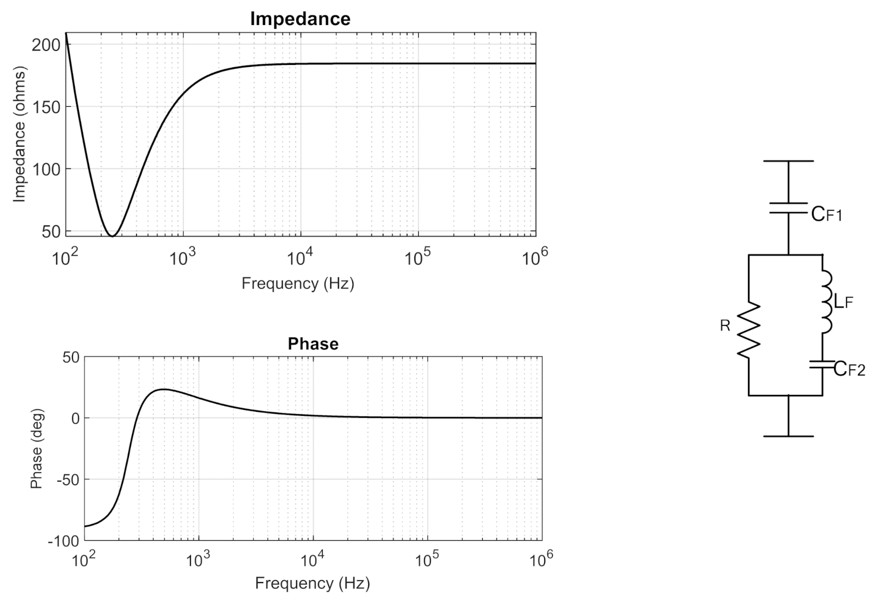
The simplest type of harmonic passive filter is the 1st order filter which is comprised of a capacitor in series with a resistor. The capacitor is used to provide capacitive reactance for $DPF$ correction, and the resistor provides the damping characteristic. The second order filter is comprised of an inductor in parallel with a resistor R, and the resulted circuit is in series with the capacitor. High power loss is the disadvantage of these two mentioned filters, and basically, to get better harmonic filtering performance, the tuned filters with further reduction of the fundamental power losses were implemented, which are named the third order passive filter and the C-type passive third order filter, and operate as a single-tuned filter at low frequencies below the tuning one; therefore, the fundamental loss has been reduced. At high frequencies, above the tuning frequency, the filter will operate as the 1st order harmonic passive filters. The C-type filter has no fundamental loss and is below the tuning frequency, therefore it acts as the 2nd order filters. At high frequencies, above the tuning frequency, the filter will operate in a similar manner to the first order harmonic passive filters [37].

According to the above explanation, the performance of these two types of third order harmonic filters will be compared for scenario 1.

Table 8. Impact on the designed filter on the system performance.

	No Filter	C-Type Filter	Third Order Filter
$I_S(pu)$	0.9596	0.7642	0.7732
$V_{PCC}(pu)$	0.9927	0.9997	0.9989
$V_L(pu)$	0.9728	0.9957	0.9949
$TPF(\%)$	69.0024	98.56	97.96
$DPF(\%)$	73.1726	99.96	98.99
$P{F}_L(\%)$	70.2339	92.63	91.85
$P{F}_{HA}(\%)$	45.1853	91.56	90.84
$MLL(\%)$	4.4511	1.34	1.54
$THD{V}_L(\%)$	15.0626	3.17	3.56
$THD{V}_{PCC}(\%)$	4.1633	3.58	3.64
$TDD(\%)$	23.7984	8.95	9.15
$\eta (\%)$	94.75	99.83	99.03

shows the impact of the designed filters using the AOA on the system performance. Besides, the uncompensated system results are included for comparison. By using the third order filter and C-type filters, respectively, it can be noticed that $P{F}_L(\%)$ is improved from 70.2339% to 91.85% and 92.63%, and $P{F}_{HA}(\%)$ is increased from 45.1853% to 92.63% and 91.56%. $\eta (\%)$ is increased from 94.75.7 to 99.83 and 99.03%, respectively. Furthermore, all three filters provide almost the same $THDV$ and $TDD$ values below the standard thresholds. Lastly, with the employment of third order and C-Type filters, $I_S(pu)$ is decreased from 0.9596 to 0.7732 and 0.7642, respectively, and $V_L(pu)$ is increased from 0.9728 to 0.9949 and 0.9957, respectively. This means that for the effective utilization of the lines, the C-type filter accomplishes improved performance compared to another filter. Besides, the comparative analysis validates that the C-type filter provides a higher power factor, system efficiency and transmission loss improvement than the third order filter.

5. Discussion

In this paper, mathematical modeling is proposed and explained using the Archimedes optimization algorithm to optimize the C-type passive filter parameters based on the new POF. In the POF, both losses of the transmission line and load bus are considered. The findings are as follows:

• The POF optimizes the CTF parameters based on the normalized transmission line loss and normalized loads bus losses, which includes fundamental and harmonic losses.
• The AOA is an effective optimization. Concerning convergence speed and the exploration–exploitation equilibrium, it can solve complex problems. The proposed method is compared with the results in the previous publication which was implemented in the Harris Hawks optimization algorithm. The filter is designed to get the optimum solution satisfying the proposed individual objective for the harmonic power loss minimization while considering the nonlinear loads, the voltage source harmonic, and current distortion. The qualified studies confirm that the proposed technique signifies a useful tool with better precision and effectiveness of the developed algorithm to achieve the best solution from a certain situation.
• The obtained results show that the implemented optimization algorithm can reduce the total harmonic distortion according to the IEEE standard threshold.
• By using the CTF, it can be noticed that $P{F}_L(\%)$ for scenario 1 and scenario 2 is improved from 70.23% to 92.63%, and from 68.27% to 87.49%, respectively.
• By using the CTF, $THDV$ and $THDI$ have been improved compared to the uncompensated system for both scenarios.
• Comparing results of the POF and the represented function in [29] shows that less reactive power must be injected into the system by the proposed method. In addition, the network efficiency and $TPF$ have increased 0.81% and 0.61%, respectively, compared to the OF in [29].
• The comparative analysis validates that the C-type filter provides a higher power factor, system efficiency and transmission loss improvement than the third order filter.

References

1. Sakar, S.; Balci, M.E.; Aleem, S.H.A.; Zobaa, A.F. Increasing PV hosting capacity in distorted distribution systems using passive harmonic filtering. Electr. Power Syst. Res. 2017, 148, 74–86. [Google Scholar] [CrossRef] [Green Version]
2. Sadati, S.B.; Yazdani-Asrami, M.; Taghipour, M. Effects of harmonic current content and ambient temperature on load ability and life time of distribution transformers. Int. Rev. Electr. Eng. 2010, 5, 1444–1451. [Google Scholar]
3. Rönnberg, S.; Bollen, M.H.; Amaris, H.; Chang, G.W.; Gu, I.Y.; Kocewiak, H.; Meyer, J.; Olofsson, M.; Ribeiro, P.; Desmet, J. On waveform distortion in the frequency range of 2–150 kHz—Review and research challenges. Electr. Power Syst. Res. 2017, 150, 1–10. [Google Scholar] [CrossRef]
4. Yazdani-Asrami, M.; Sadati, S.M.B.; Samadaei, E. Harmonic study for MDF industries: A case study. In Proceedings of the 2011 IEEE Applied Power Electronics Colloquium (IAPEC), Johor Bahru, Malaysia, 18–19 April 2011; pp. 149–154. [Google Scholar]
5. Das, J.C. Power System Harmonics and Passive Filter Designs; John Wiley & Sons: Hoboken, NJ, USA, 2015. [Google Scholar] [CrossRef]
6. Karadeniz, A.; Balci, M.E. Comparative evaluation of common passive filter types regarding maximization of transformer’s loading capability under non-sinusoidal conditions. Electr. Power Syst. Res. 2018, 158, 324–334. [Google Scholar] [CrossRef]
7. Yazdani-Asrami, M.; Mirzaie, M.; Akmal, A.S. Calculation of transformer losses under non-sinusoidal currents using: Two analytic methods and finite element analysis. World Appl. Sci. J. 2010, 9, 889–897. [Google Scholar]
8. Khodsuz, M.; Sheikholeslami, A. Voltage improvement and harmonic compensation in stand-alone inverter-based distributed generation using RS-HNSPWM. In Proceedings of the 2009 2nd International Conference on Power Electronics and Intelligent Transportation System (PEITS), Shenzhen, China, 19–20 December 2009; Volume 1, pp. 50–55. [Google Scholar] [CrossRef]
9. Yazdani-Asrami, M.; Song, W.; Zhang, M.; Yuan, W.; Pei, X. AC Transport Loss in Superconductors Carrying Harmonic Current with Different Phase Angles for Large-Scale Power Components. IEEE Trans. Appl. Supercond. 2020, 31, 1–5. [Google Scholar] [CrossRef]
10. Leite, J.C.; Abril, I.P.; Tostes, M.E.D.L.; De Oliveira, R.C.L. Multi-objective optimization of passive filters in industrial power systems. Electr. Eng. 2017, 99, 387–395. [Google Scholar] [CrossRef]
11. Yazdani-Asrami, M.; Song, W.; Pei, X.; Zhang, M.; Yuan, W. AC Loss Characterization of HTS Pancake and Solenoid Coils Carrying Nonsinusoidal Currents. IEEE Trans. Appl. Supercond. 2020, 30, 1–9. [Google Scholar] [CrossRef] [Green Version]
12. Yazdani-Asrami, M.; Mirzaie, M.; Akmal, A.S.; Gholamian, S.A. Life Estimation of Distribution Transformers Under Non-Linear Loads Using Calculated Loss by 2D-FEM. J. Electr. Syst. 2011, 7, 12–24. [Google Scholar]
13. Song, W.; Fang, J.; Jiang, Z. Numerical AC Loss Analysis in HTS Stack Carrying Nonsinusoidal Transport Current. IEEE Trans. Appl. Supercond. 2018, 29, 1–5. [Google Scholar] [CrossRef]
14. Yazdani-Asrami, M.; Taghipour-Gorjikolaie, M.; Song, W.; Zhang, M.; Yuan, W. Prediction of Nonsinusoidal AC Loss of Superconducting Tapes Using Artificial Intelligence-Based Models. IEEE Access 2020, 8, 207287–207297. [Google Scholar] [CrossRef]
15. Yazdani-Asrami, M.; Song, W.; Zhang, M.; Yuan, W.; Pei, X. Magnetization Loss in HTS Coated Conductor Exposed to Harmonic External Magnetic Fields for Superconducting Rotating Machine Applications. IEEE Access 2021, 9, 77930–77937. [Google Scholar] [CrossRef]
16. Song, W.; Fang, J.; Jiang, Z.; Staines, M.; Badcock, R. AC Loss Effect of High-Order Harmonic Currents in a Single-Phase 6.5 MVA HTS Traction Transformer. IEEE Trans. Appl. Supercond. 2019, 29, 1–5. [Google Scholar] [CrossRef]
17. Yazdani-Asrami, M.; Gholamian, S.A.; Mirimani, S.M.; Adabi, J. Influence of field-dependent critical current on harmonic AC loss analysis in HTS coils for superconducting transformers supplying non-linear loads. Cryogenics 2020, 113, 103234. [Google Scholar] [CrossRef]
18. Bagheri, P.; Xu, W. A Technique to Mitigate Zero-Sequence Harmonics in Power Distribution Systems. IEEE Trans. Power Deliv. 2014, 29, 215–223. [Google Scholar] [CrossRef]
19. El-Ela, A.A.; Allam, S.; El-Arwash, H. An optimal design of single tuned filter in distribution systems. Electr. Power Syst. Res. 2008, 78, 967–974. [Google Scholar] [CrossRef]
20. Teke, A.; Saribulut, L.; Tumay, M. A Novel Reference Signal Generation Method for Power-Quality Improvement of Unified Power-Quality Conditioner. IEEE Trans. Power Deliv. 2011, 26, 2205–2214. [Google Scholar] [CrossRef]
21. Ghorbani, A. An adaptive distance protection scheme in the presence of phase shifting transformer. Electr. Power Syst. Res. 2015, 129, 170–177. [Google Scholar] [CrossRef]
22. Yang, Z.; Sun, J.; Li, S.; Huang, M.; Zha, X.; Tang, Y. An adaptive Carrier frequency optimization method for harmonic energy unbalance minimization in a cascaded HBridge-Based active power filter. IEEE Trans. Power Electron. 2018, 33, 1024–1037. [Google Scholar] [CrossRef]
23. Khodsuz, M.; Sheikholeslami, A. Voltage regulation and harmonic compensation in stand-alone inverter-based distributed generation using non-sinusoidal hysteresis voltage control. In Proceedings of the 2009 2nd International Conference on Power Electronics and Intelligent Transportation System (PEITS), Shenzhen, China, 19–20 December 2009; Volume 1, pp. 44–49. [Google Scholar] [CrossRef]
24. Elbasuony, G.S.; Aleem, S.H.A.; Ibrahim, A.M.; Sharaf, A.M. A unified index for power quality evaluation in distributed generation systems. Energy 2018, 149, 607–622. [Google Scholar] [CrossRef]
25. Mahanty, R. Large value AC capacitor for harmonic filtering and reactive power compensation. IET Gener. Transm. Distrib. 2008, 2, 876–891. [Google Scholar] [CrossRef]
26. Marzoughi, A.; Imaneini, H.; Moeini, A. An optimal selective harmonic mitigation technique for high power converters. Int. J. Electr. Power Energy Syst. 2013, 49, 34–39. [Google Scholar] [CrossRef]
27. Choi, W.-H.; Lam, C.-S.; Wong, M.-C.; Han, Y.-D. Analysis of DC-Link Voltage Controls in Three-Phase Four-Wire Hybrid Active Power Filters. IEEE Trans. Power Electron. 2013, 28, 2180–2191. [Google Scholar] [CrossRef]
28. Ismael, S.M.; Aleem, S.H.E.A.; Abdelaziz, A.Y.; Zobaa, A.F. State-of-the-art of hosting capacity in modern power systems with distributed generation. Renew Energy 2019, 130, 1002–1020. [Google Scholar] [CrossRef]
29. Aleem, S.H.E.A.; Zobaa, A.F.; Balci, M.E.; Ismael, S.M. Harmonic Overloading Minimization of Frequency-Dependent Components in Harmonics Polluted Distribution Systems Using Harris Hawks Optimization Algorithm. IEEE Access 2019, 7, 100824–100837. [Google Scholar] [CrossRef]
30. Upadhye, S.; Atre, Y.F. Determination of the design parameters of passive harmonic filters using nonlinear optimization. In Proceedings of the 1998 IEEE Industrial and Commercial Power Systems Technical Conference, Edmonton, AB, Canada, 3–8 May 1998; pp. 155–164. [Google Scholar]
31. Aleem, S.H.A.; Elmathana, M.T.; Zobaa, A.F. Different Design Approaches of Shunt Passive Harmonic Filters Based on IEEE Std. 519-1992 and IEEE Std. 18-2002. Recent Pat. Electr. Electron. Eng. 2013, 6, 68–75. [Google Scholar] [CrossRef]
32. Singh, N.S.P.; Nair, N.K. Artificial bee colony algorithm for inverter complex wave reduction under line-load variations. Trans. Inst. Meas. Control 2017, 40, 1593–1607. [Google Scholar] [CrossRef]
33. Mohammadi, N.A.; Rozbahani, A.M.; Montazeri, M. Multi criteria simultaneous planning of passive filters and distributed generation simultaneously in distribution system considering nonlinear loads with adaptive bacterial foraging optimization approach. Int. J. Electr. Power Energy Syst. 2016, 79, 253–262. [Google Scholar] [CrossRef]
34. Biswas, P.P.; Suganthan, P.; Amaratunga, G.A. Minimizing harmonic distortion in power system with optimal design of hybrid active power filter using differential evolution. Appl. Soft Comput. 2017, 61, 486–496. [Google Scholar] [CrossRef]
35. Dhabal, S.; Venkateswaran, P. An efficient gbest-guided Cuckoo Search algorithm for higher order two channel filter bank design. Swarm Evol. Comput. 2017, 33, 68–84. [Google Scholar] [CrossRef]
36. Aleem, S.H.A.; Zobaa, A.F.; Balci, M.E. Optimal resonance-free third-order high-pass filters based on minimization of the total cost of the filters using Crow Search Algorithm. Electr. Power Syst. Res. 2017, 151, 381–394. [Google Scholar] [CrossRef] [Green Version]
37. Yang, N.; Le, M. Multi-objective bat algorithm with time-varying inertia weights for optimal design of passive power filters set. IET Gener. Transm. Distrib. 2015, 9, 644–654. [Google Scholar] [CrossRef]
38. Abril, I.P. Passive filters’ placement considering parameters’ variations. Int. Trans. Electr. Energy Syst. 2018, 29, e2727. [Google Scholar] [CrossRef]
39. Jeon, S.-J. Non-sinusoidal power theory in a power system having transmission lines with frequency-dependent resistances. IET Gener. Transm. Distrib. 2007, 1, 331–339. [Google Scholar] [CrossRef]
40. Hiranandani, A. Calculation of cable ampacities including the effects of harmonics. IEEE Ind. Appl. Mag. 1998, 4, 42–51. [Google Scholar] [CrossRef]
41. Bagheri, P.; Xu, W.; Shaloudegi, K. New indices to evaluate the impact of harmonic currents on power transformers. In Proceedings of the 2018 18th International Conference on Harmonics and Quality of Power (ICHQP) 2018, Ljubljana, Slovenia, 13–16 May 2018; pp. 1–6. [Google Scholar] [CrossRef]
42. Hashim, F.A.; Hussain, K.; Houssein, E.H.; Mabrouk, M.S.; Al-Atabany, W. Archimedes optimization algorithm: A new metaheuristic algorithm for solving optimization problems. Appl. Intell. 2021, 51, 1531–1551. [Google Scholar] [CrossRef]
43. Wang, Y.; Xu, S.; Xu, W.; Wu, J.; Xiao, X. Comparative Studies on Design Methods for Detuned C-Type Filter. IEEE Trans. Power Deliv. 2019, 35, 1725–1734. [Google Scholar] [CrossRef]
44. Balci, M.E.; Emanuel, A.E. Apparent power definitions: A comparison study. Int. Rev. Electr. Eng. 2011, 6, 2713–2722. [Google Scholar]
45. McEachern, A.; Grady, W.; Moncrief, W.; Heydt, G.; McGranaghan, M. Revenue and harmonics: An evaluation of some proposed rate structures. IEEE Trans. Power Deliv. 1995, 10, 474–482. [Google Scholar] [CrossRef]
46. IEEE Std. 519-2014; IEEE Recommended Practices and Requirements for Harmonic Control in Electrical Power Systems. IEEE: New York, NY, USA, 2014.
Figure 1. The C-type filter (CTF) single-phase equivalent circuit.
Energies 15 01587 g001
Figure 2. The CTF design situations.
Energies 15 01587 g002
Figure 3. Single-phase equivalent circuit given.
Energies 15 01587 g003
Figure 4. Working flowchart of the Archimedes optimization algorithm (AOA).
Energies 15 01587 g004
Figure 5. The schematic diagram of the proposed technique.
Energies 15 01587 g005
Figure 6. The threshold values according to the IEEE 519.
Energies 15 01587 g006
Figure 7. The convergence rate in finding the best fitness.
Energies 15 01587 g007
Figure 8. The individual harmonic voltage and current distortion values—scenario 1.
Energies 15 01587 g008
Figure 9. The individual harmonic voltage and current distortion values—scenario 2.
Energies 15 01587 g009
Figure 10. Obtained values based on the proposed OF in [29] by the AOA algorithm (a) I H D V P C C , (b) I H D V L , (c) I H D I .
Energies 15 01587 g010