
Time-Interval-Varying Optimal Power Dispatch Strategy Based on Net Load Time-Series Characteristics

 ,
,
Abstract
:
1. Induction
2. Time-Series Characteristics Analysis of Net Loads Based on RMT
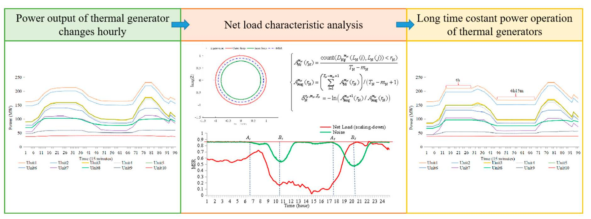
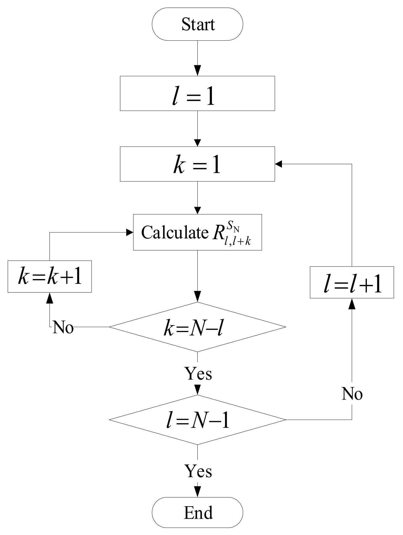
2.1. Monocyclic Theorem and the Calculation of the Mean Spectral Radius (MSR)
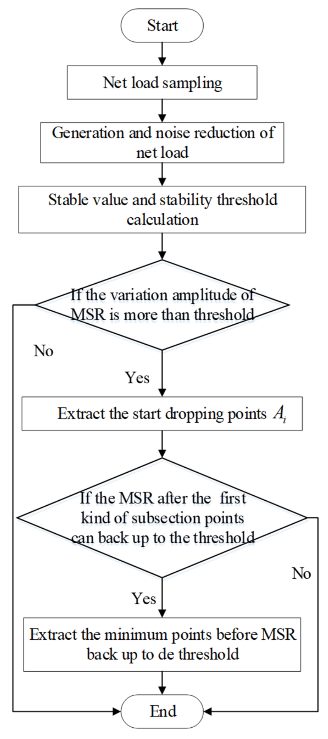
2.2. Time Interval Division Method of Net Load
3. Quantification of Net Load Time-Series Characteristics
3.1. Numerical Characteristic Analysis Based on EMD
- (1)
- Extract the maximum points and their fitting envelope curve of the original time series ;
- (2)
- Extract the minimum points and their fitting envelope curve ;
- (3)
- Calculate the average value of the up- and low-fitting envelope curves; which can be calculated as
- (4)
- Update the net load time series with the equation , and repeat Step (1) until the satisfies the constraints of IMF. The IMF has two constraints, the first is the numerical difference between the extreme points number and zero crossing points number, which is not more than 1; the second is that at any point the average value of the up- and low-fitting envelope curves is 0. The is the first IMF component that contains the highest frequency components.
- (5)
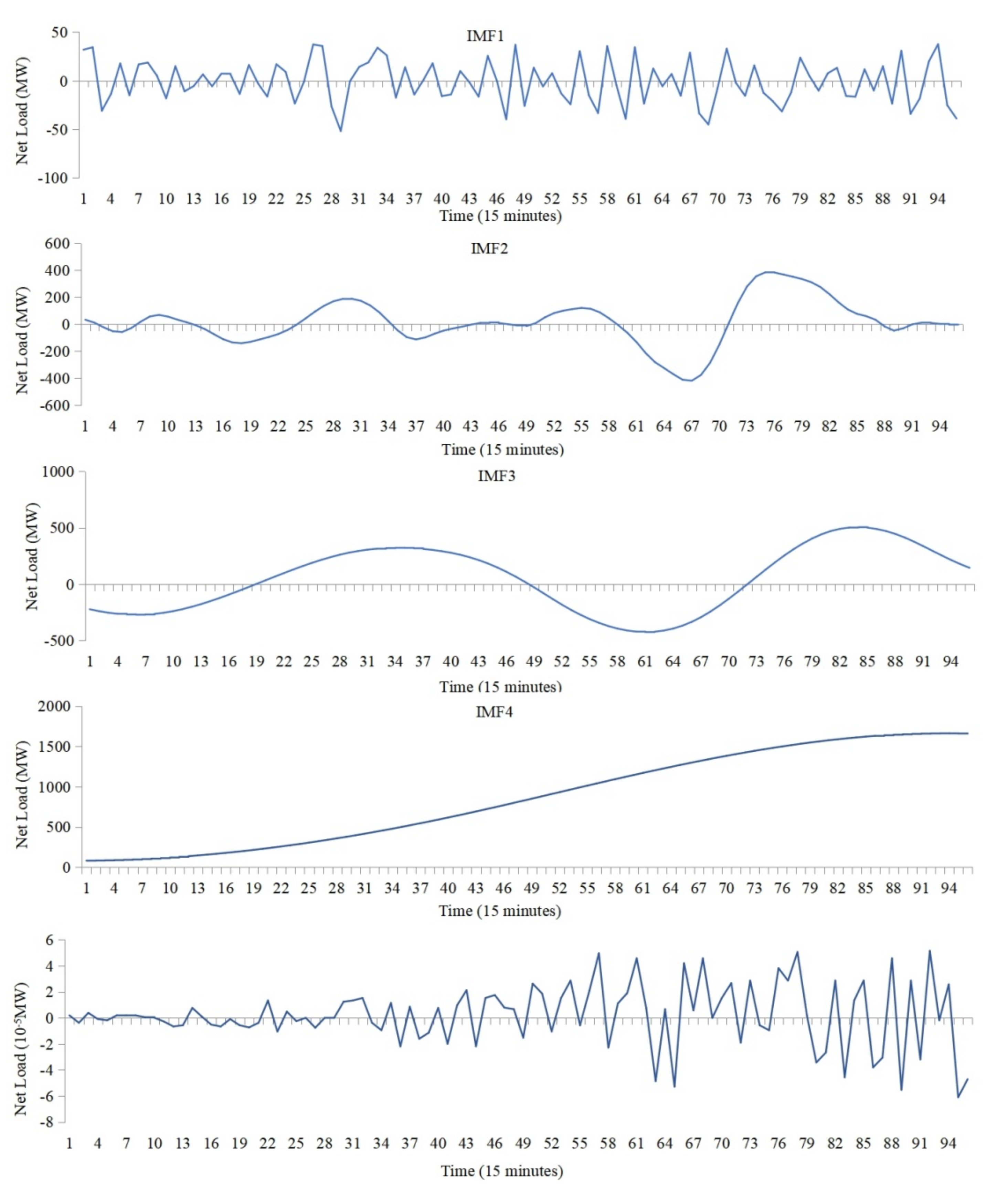
- Extract the component of IMF from the original signal , and the remaining components are formulated as .
- (6)
- Set the remaining components as the new original signal and repeat the steps above. The other components of IMF and a margin can be achieved, which can be shown as follows:
3.2. Numerical Characteristic Calculation
3.3. Net Load Complexity Calculation
3.4. Quantification of the Net Load Time-Series Characteristics
- (1)
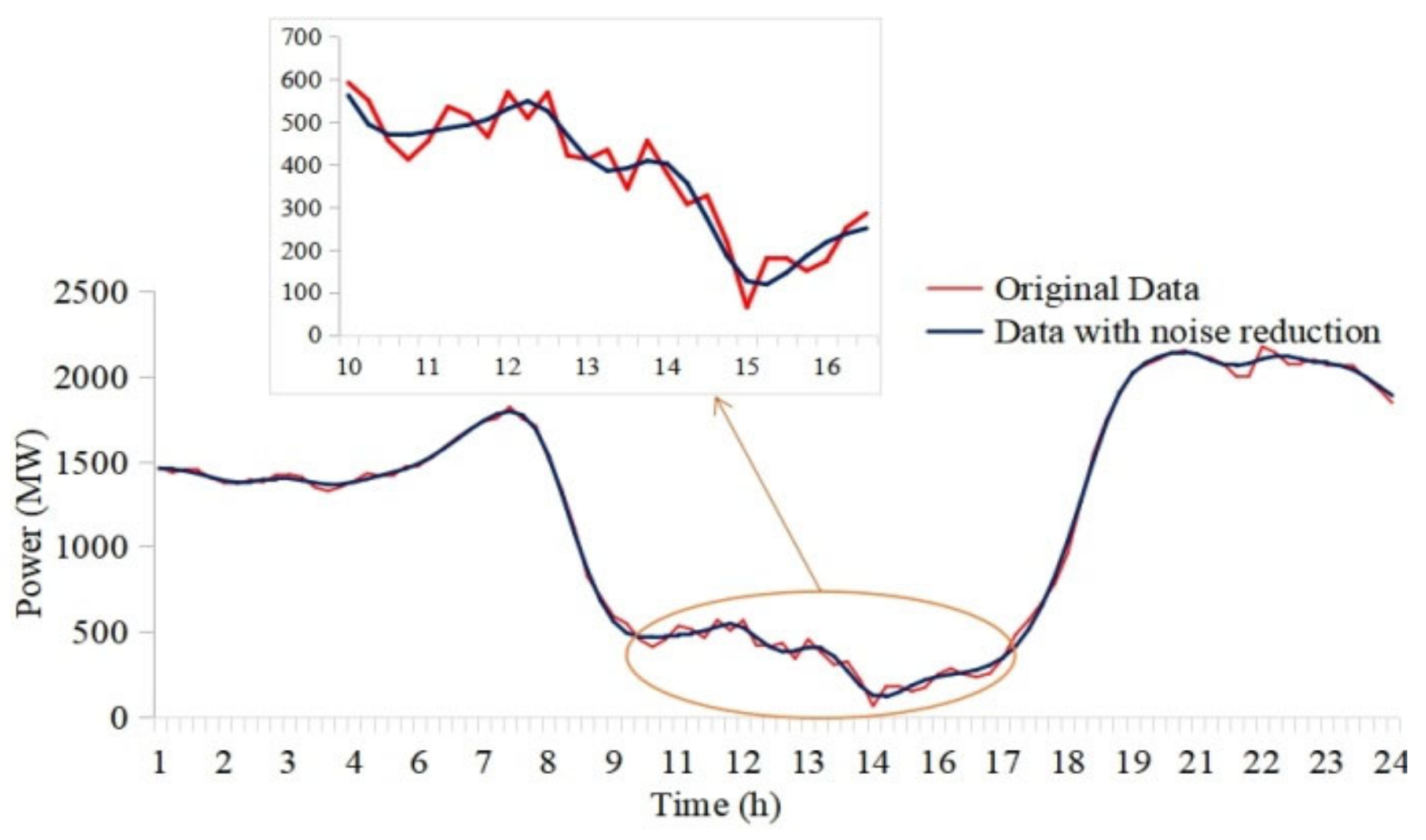
- Decompose the net load curve based on EMD and extract the noise reduction curve with the high frequency component reduction.
- (2)
- Analyze the numerical characteristic of the net load curve and calculate the ratio of slope symbol changing time to the data length.
- (3)
- Based on the net load time division results, calculate the complexity of the net load subsequence with SampEn.
- (4)
- Synthesize the time division results, numerical characteristic, and complexity; the quantitative index is calculated.
4. Time-Interval-Varying Optimal Power Dispatch Model
4.1. Time-Interval-Varying Optimal Power Dispatch Strategy Description
4.2. Time-Interval-Varying Optimal Power Dispatch Model
4.2.1. Objective Functions
4.2.2. Constraints of the Dispatch Model
Power Balance Constraints
Constraints of Thermal Power Outputs
Constraints of the Pumped Storage
Constraints of BES
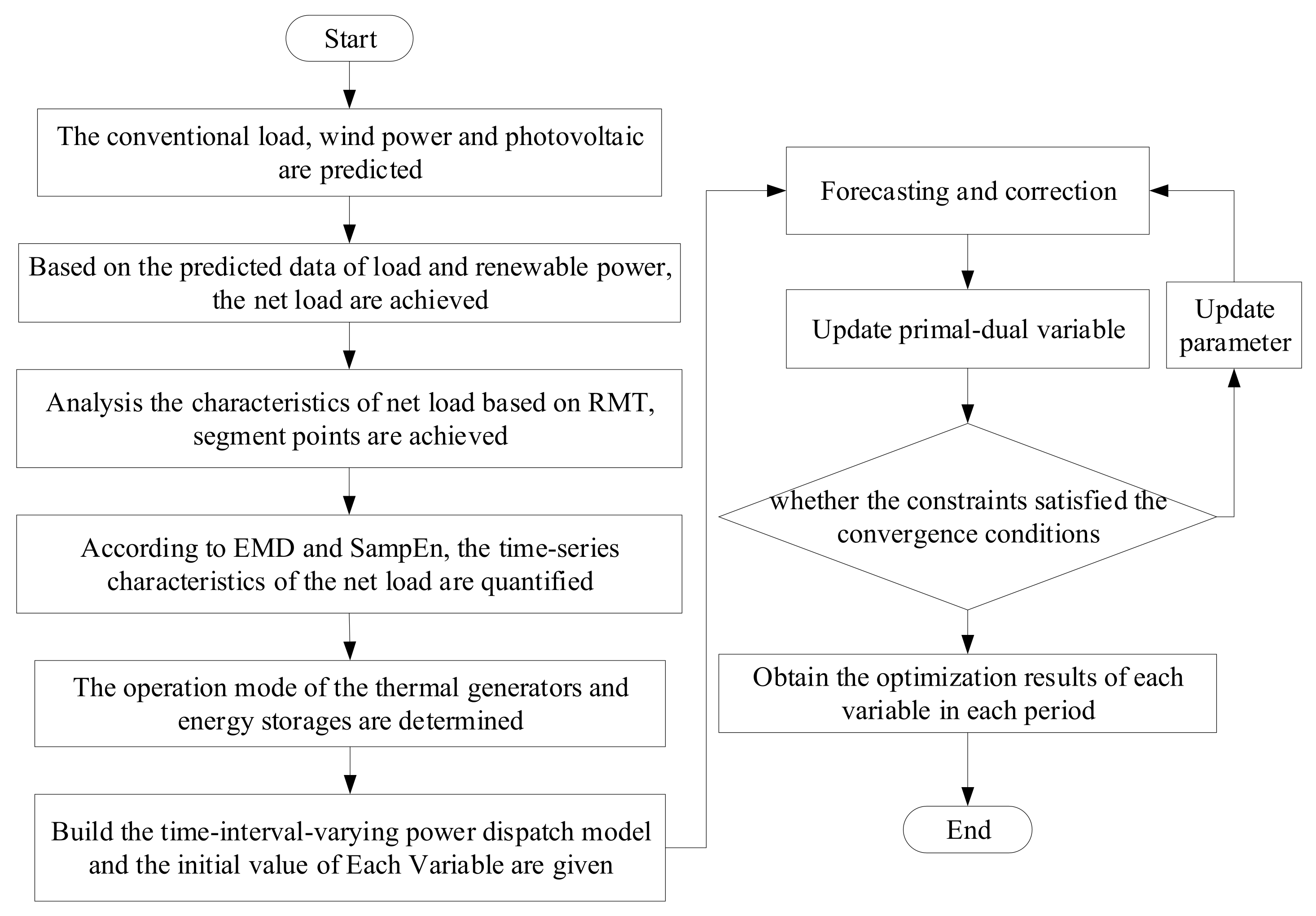
4.3. The Solving Algorithm and Process
5. Case Study
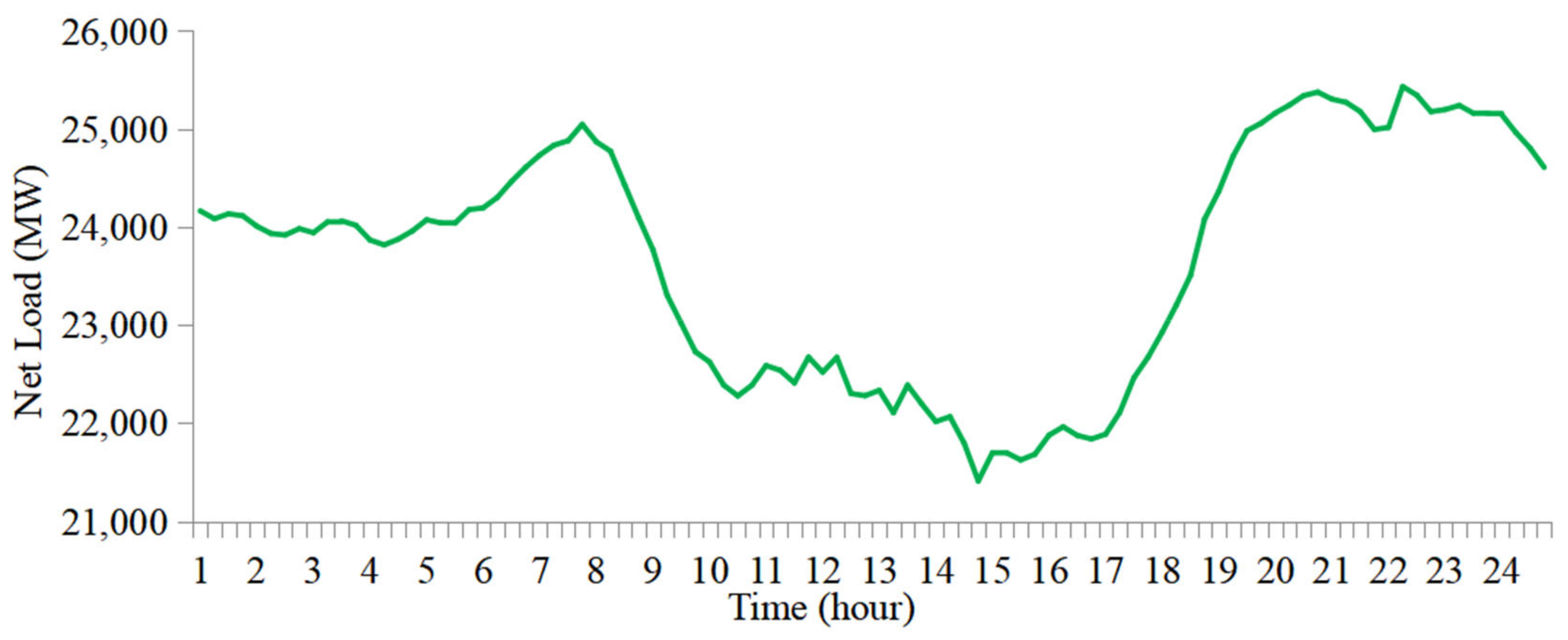
5.1. Data of the Provincial Power Grid
5.2. Time-Series Characteristic of the Provincial Net Load
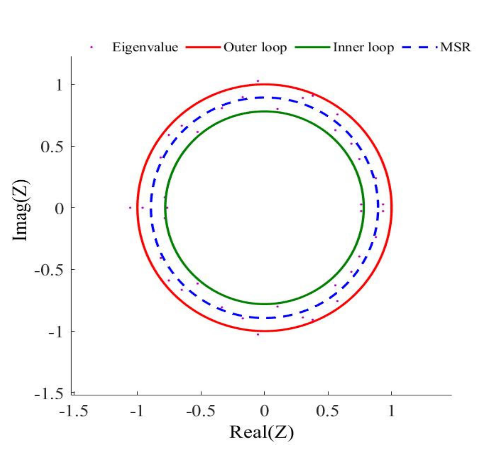
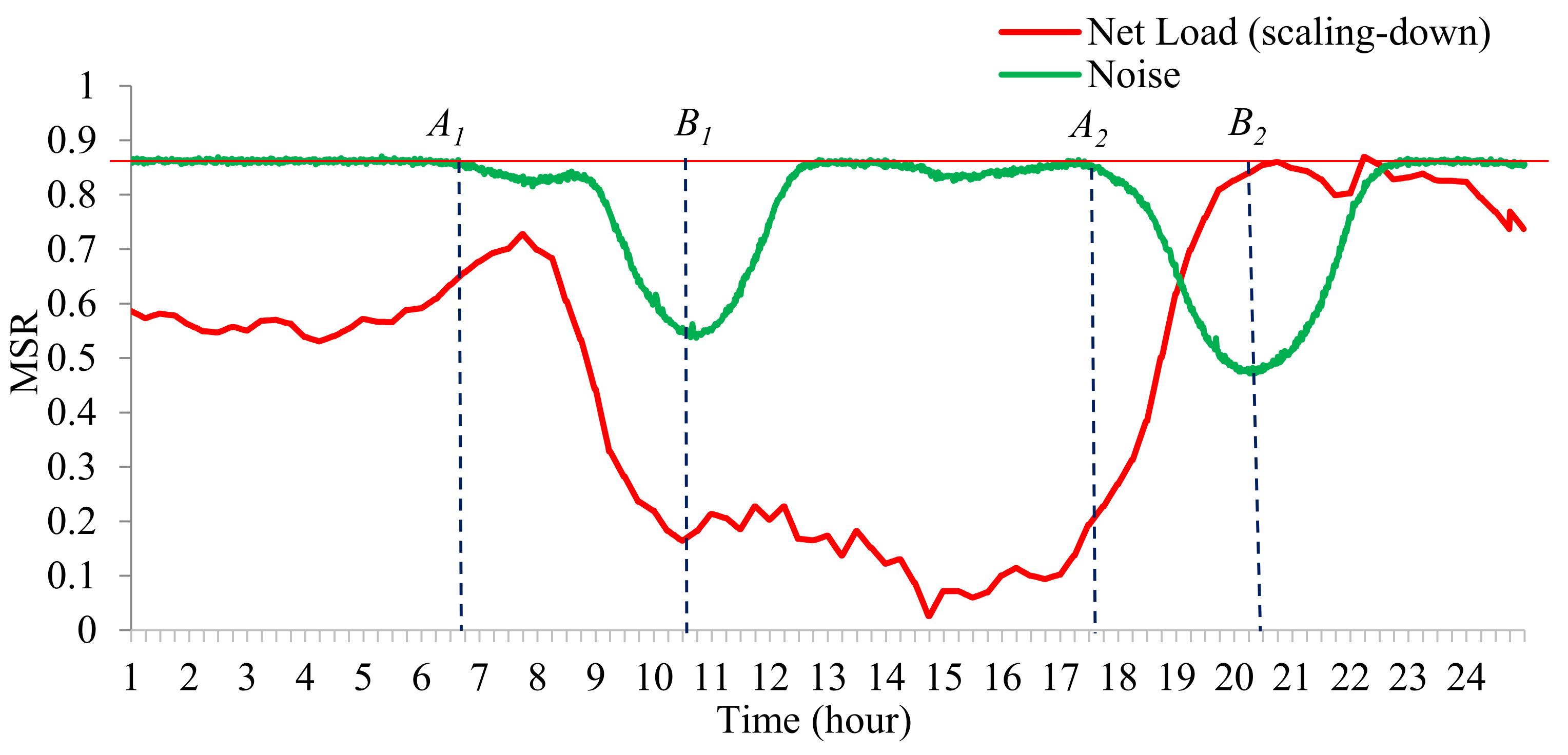
5.2.1. Time Division Based RMT
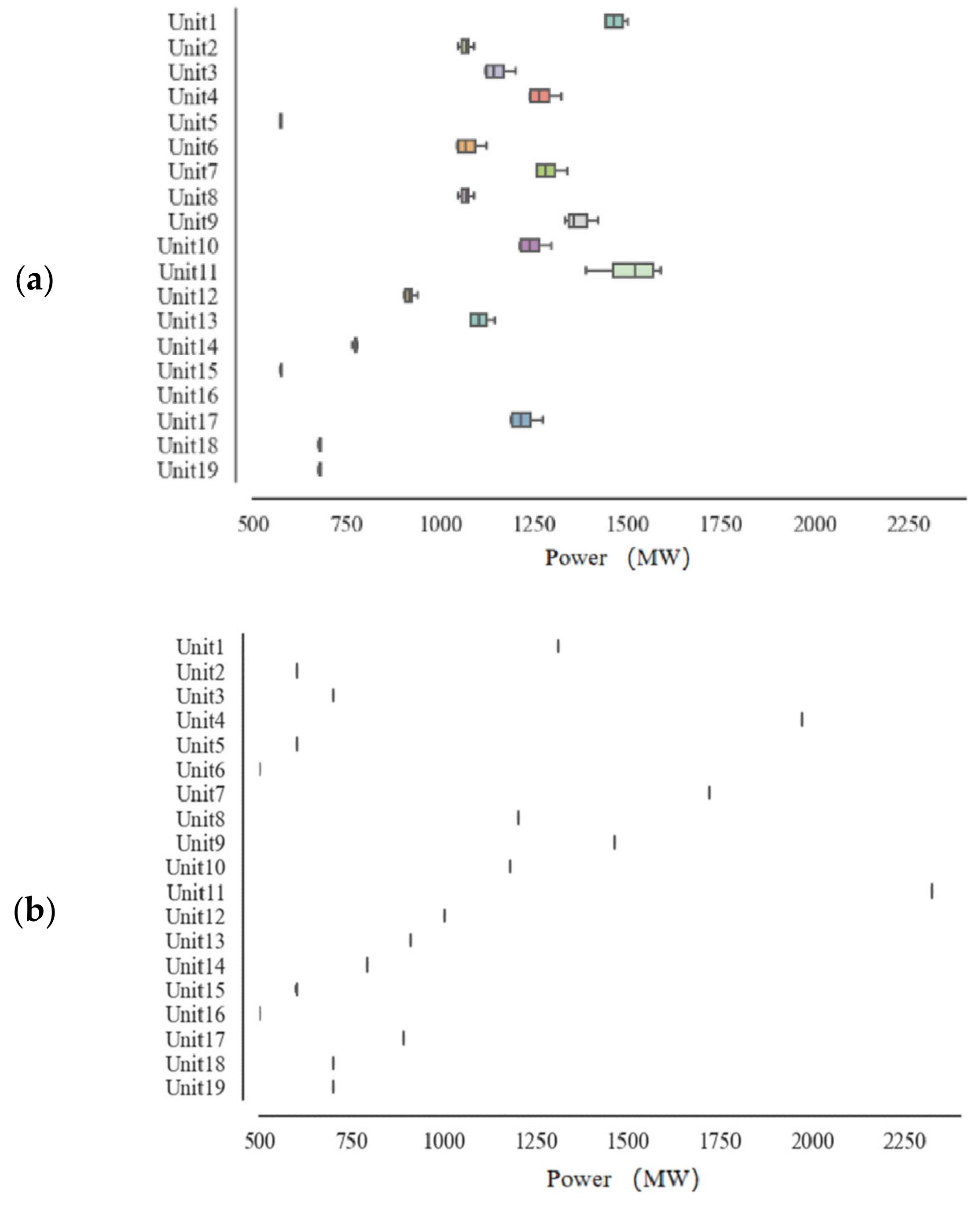
5.2.2. Characteristic Analysis of the Each Subseries
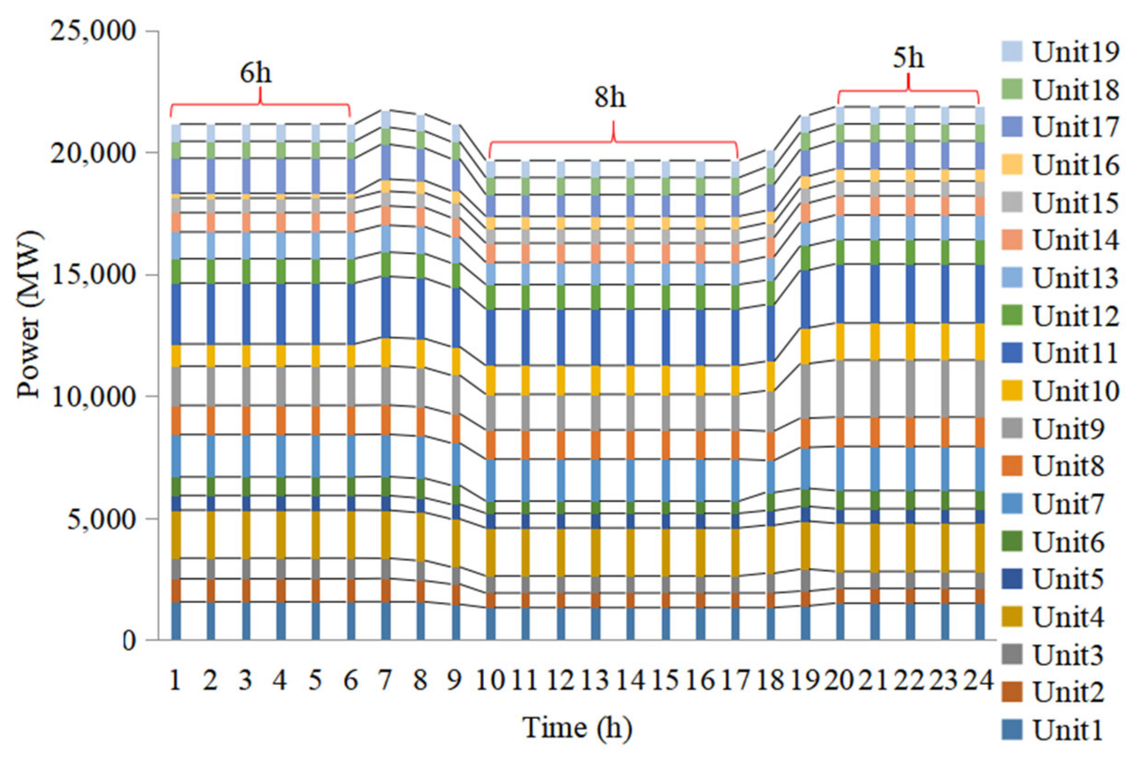
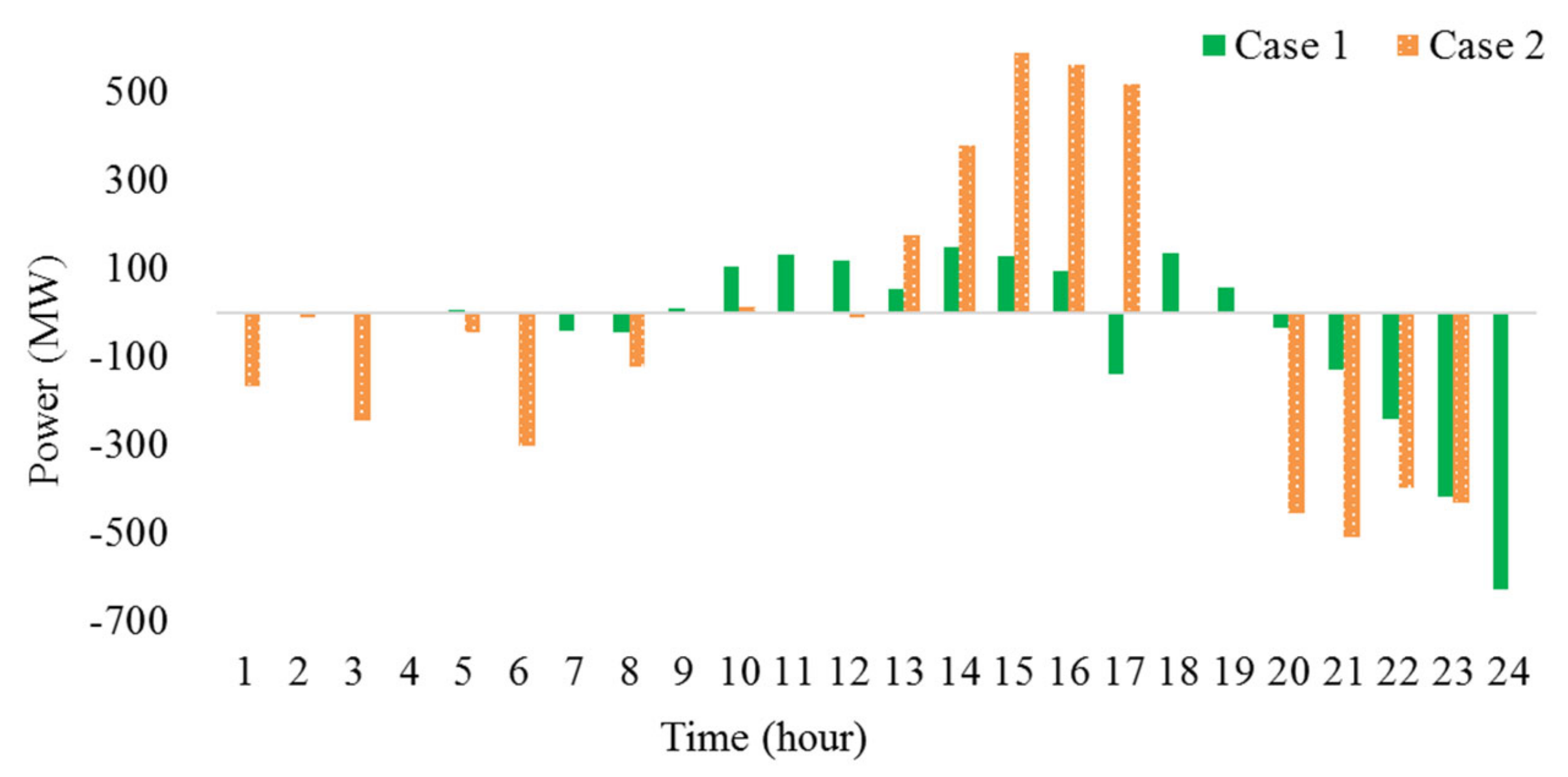
5.3. Time-Interval-Varying Dispatch Results and Benefits Analysis
- Case 1: The provincial power dispatch under the existing conventional dispatch mode;
- Case 2: The provincial power dispatch under the proposed time-interval-varying net load power dispatch mode.
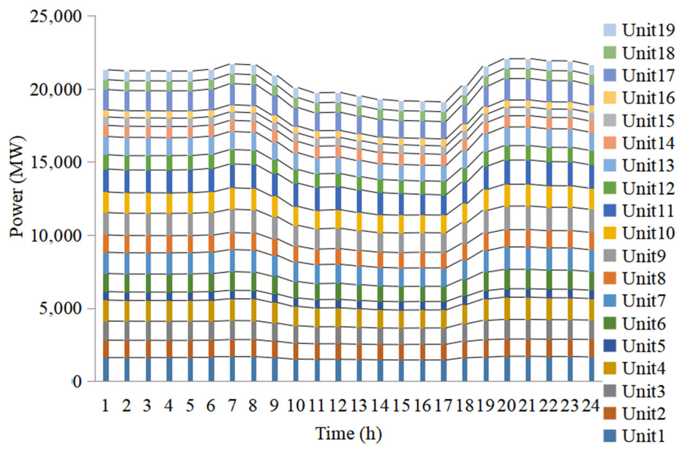
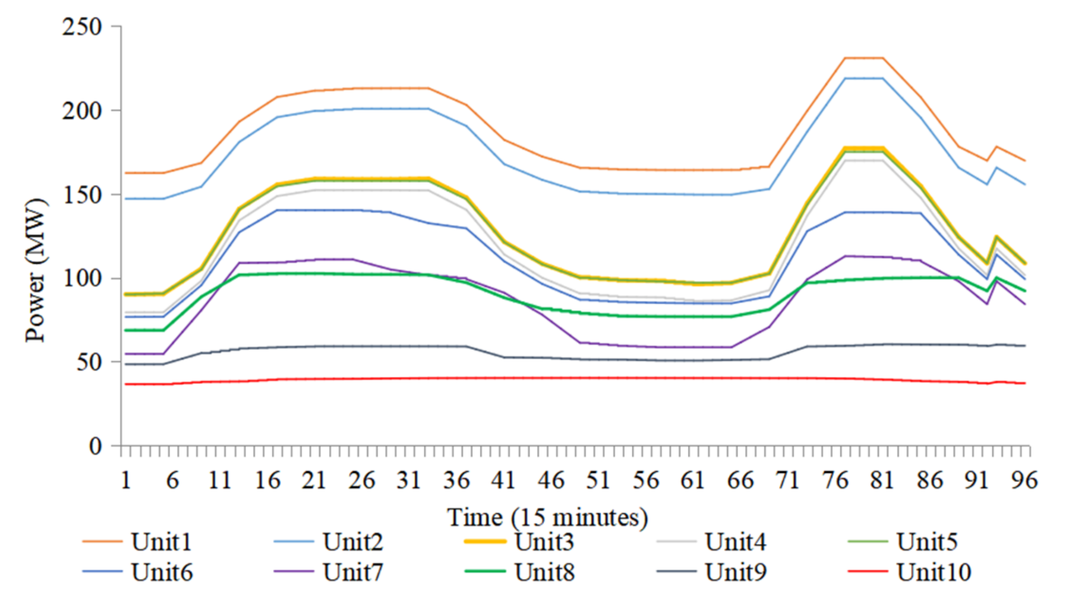
5.3.1. Dispatch Result Analysis of the Two Cases
5.3.2. Environmental Benefit Analysis
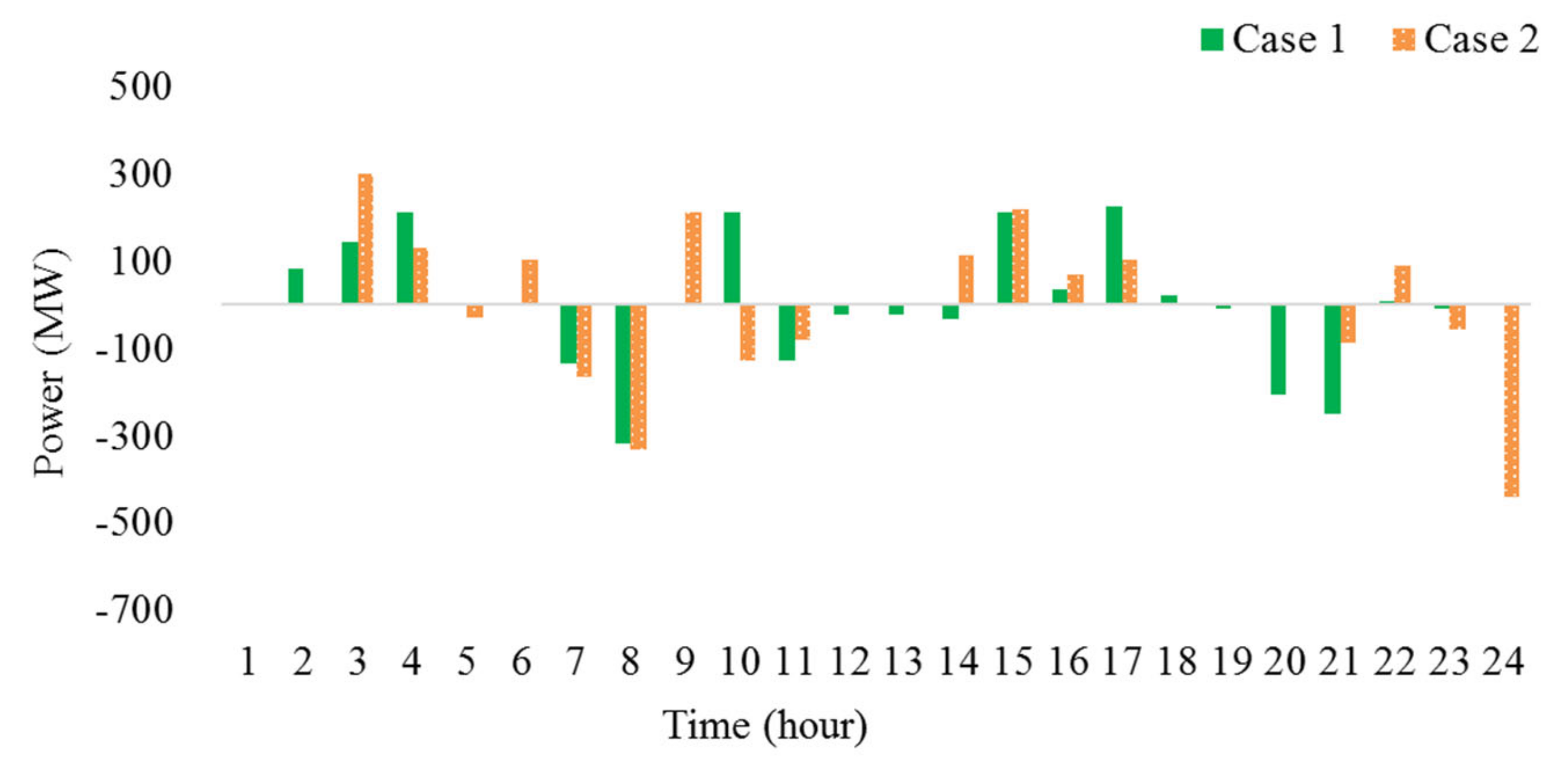
5.4. Case Study Based on the IEEE 39 System
Discussion Based on the Provincial Power System
- Case 3: Power dispatch under the existing conventional dispatch mode;
- Case 4: Power dispatch under the proposed time-interval-varying net load power dispatch mode.
5.5. Discussion
5.5.1. Discussion Based on the Provincial Power System
5.5.2. Discussion Based on the IEEE 39 System
6. Conclusions
- (1)
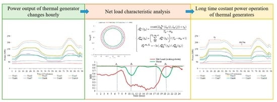
- A time-interval-varying power dispatch method is proposed, in which the net load time-series characteristics are analyzed by the RMT and the time intervals are divided adaptively. The number and length of the time intervals are determined by net loads accordingly.
- (2)
- A net load time-series characteristic quantification method is proposed. The net loads have different characteristics in each time interval. The EMD and SampEn are combined to analyze the fluctuation and complexity of the net load subsequence. A comprehensive characteristic quantification index integrated with the numerical characteristic and complexities is provided. The maximum index can reflect the fluctuation and complexity of the net loads, which can help with the data-mode fusion in the dispatch mode determination.
- (3)
- A time-interval-varying power dispatch method is developed to maximize the utilization of the wind power. According to the time division results and quantification characteristics in each time interval, the operation mode of thermal generators and energy storage systems are determined.
- (4)
- An actual provincial power grid in northeast China is used to conduct the proposed method. In Case 2, time is divided into five intervals. The operation mode of thermal generators is optimized to “6-3-8-2-5” operation mode. There are three time intervals that can realize steady operation during which the thermal generators have constant power outputs. Steady operation lasts for 19 h. Benefit from the operation mode is determined based on the quantification index, the reduction of the ramping operation of the thermal generators, and the decrease of relative costs. Because of the steady operation of thermal generators, the interaction between energy storage and wind power are improved, which is beneficial to resource utilization.
- (5)
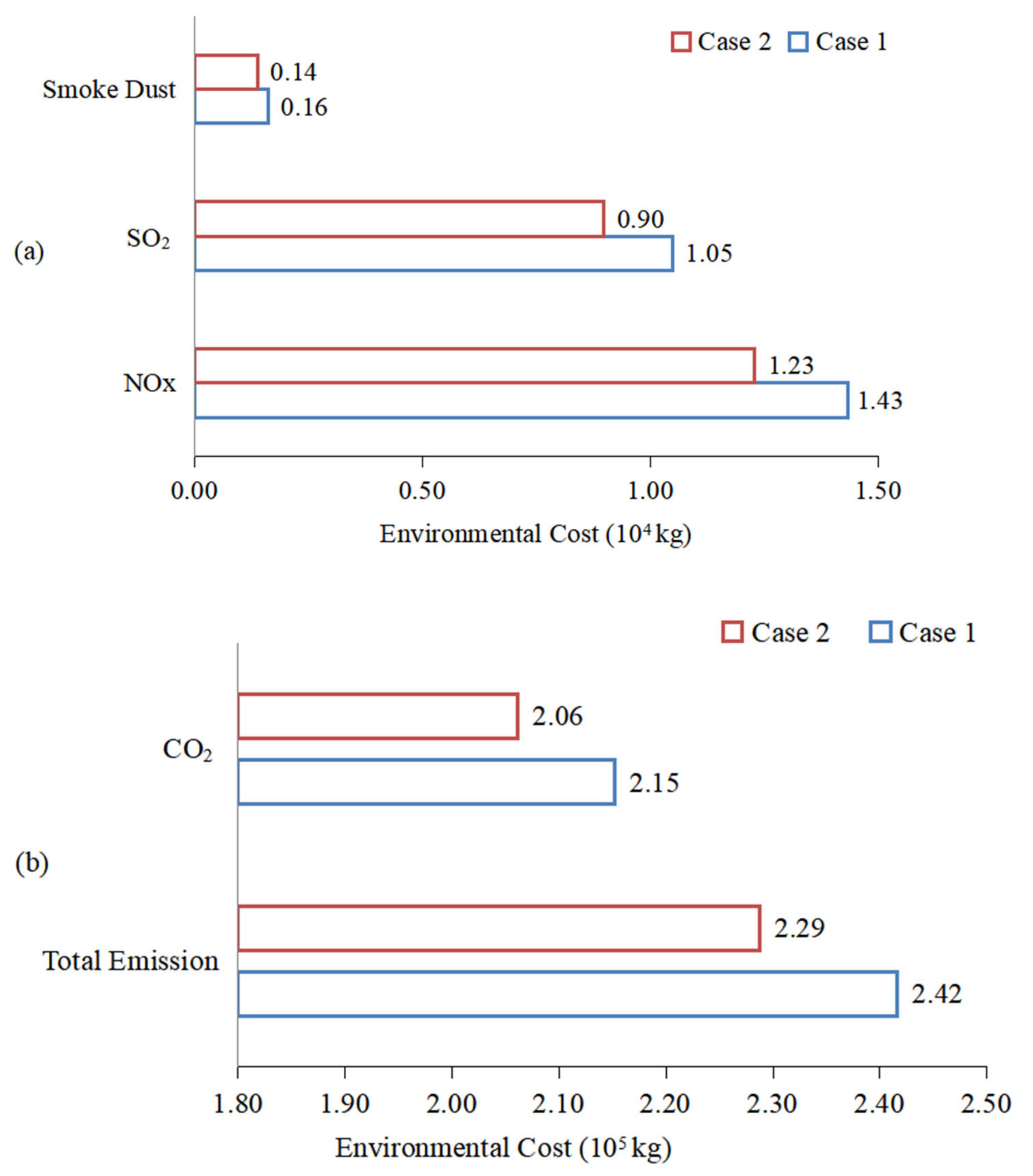
- In Case 2, the total operation cost, thermal operation cost, and ramping operation cost are all reduced. The environmental cost of CO2, NOX, SO2, and smoke dust emissions is decreased. Further, in Case 2, there are 9.06 fewer tons of carbon dioxide and 9.06 more carbon credits than those in Case 1, which certify the environmental friendliness of the proposed method and strategy.
Author Contributions
Funding
Conflicts of Interest
References
- National Energy Administration [EB/OL]. “14th Five-Year” Power Planning Work Starting. 2020-01-16. Available online: http://www.nea.gov.cn/2020-01/16/c_138709471.htm (accessed on 3 December 2020).
- Tsai, C.H.; Figueroa-Acevedo, A.; Boese, M.; Mohan, N.; Okullo, J.; Heath, B.; Bakke, J. Challenges of planning for high renewable futures: Experience in the U.S. midcontinent electricity market. Renew. Sustain. Energy Rev. 2020, 131, 109992. [Google Scholar] [CrossRef]
- Shariatmadar, K.; Arrigo, A.; Vallée, F.; Hallez, H.; Vandevelde, L.; Moens, D. Day-Ahead Energy and Reserve Dispatch Problem under Non-Probabilistic Uncertainty. Energies 2021, 14, 1016. [Google Scholar] [CrossRef]
- Li, J.H.; Wang, S.; Liu, Y.; Fang, J.K. A coordinated dispatch method with pumped-storage and battery-storage for compensating the variation of wind power. Prot. Control Mod. Power Syst. 2018, 3, 21–34. [Google Scholar] [CrossRef] [Green Version]
- Wang, W.; Xu, J.; Zhao, X.; Yuan, X.J.; Li, Z.X. Analysis on Peak Load Regulation Status Quo for Coal-fired Power Plants in China. South. Energy Constr. 2017, 4, 18–24. [Google Scholar]
- Power Plant Boiler “Burst Tube” Reason. [EB/OL]. Polaris Power Grid. 2020-06-11. Available online: https://www.sohu.com/a/401269905_752692?_trans_=010001_grzy (accessed on 1 December 2020).
- Liu, Y.; Tan, Q.; Han, J.; Guo, M. Energy-Water-Carbon Nexus Optimization for the Path of Achieving Carbon Emission Peak in China Considering Multiple Uncertainties: A Case Study in Inner Mongolia. Energies 2021, 14, 1067. [Google Scholar] [CrossRef]
- What Is Carbon Neutral? What Are the Status of Enterprises under the Carbon Neutral Vision? [EB/OL]. Polaris Electricity Selling Power Grid, 2020-11-20. Available online: http://shoudian.bjx.com.cn/html/20201120/1116972.shtml (accessed on 6 December 2020).
- Eser, P.; Singh, A.; Chokani, N.; Abhari, R.S. Effect of increased renewables generation on operation of thermal power plants. Appl. Energy 2016, 164, 723–732. [Google Scholar] [CrossRef]
- Wang, H.C.; Qin, H.; Zhou, C.; Li, F.; Xu, X.H.; Pan, X. Cross-regional Day-ahead to Intra-day Scheduling Model Considering Forecasting Uncertainty of Renewable Energy. Autom. Electr. Power Syst. 2019, 43, 60–72. [Google Scholar]
- Zhao, D.M.; Song, Y.; Wang, Y.L.; Yin, J.F.; Xu, C.L. Coordinated Scheduling Model with Multiple Time Scales Considering Response Uncertainty of Flexible Load. Autom. Electr. Power Syst. 2019, 43, 21–32. [Google Scholar]
- Galvan, E.; Gutierrez, A.G.; Gonzalez, N. Two-phase short-term scheduling approach with intermittent renewable energy resources and demand response. IEEE Lat. Am. Trans. 2015, 13, 181–187. [Google Scholar] [CrossRef]
- Achilles, S.; Schramm, S.; Bebic, J. Transmission System Performance Analysis for High-Penetration Photovoltaics; Office of Scientific & Technical Information Technical Reports; National Renewable Energy Laboratory: Golden, CO, USA, 2011. [Google Scholar]
- Hu, S.B.; Gao, Z.N.; He, H.; Cao, W.P.; Zhao, Y.T.; Zhou, W.; Gu, H.; Sun, H. Adaptive time division power dispatch based on numerical characteristics of net loads. Energy 2020, 205, 118026. [Google Scholar] [CrossRef]
- Wang, Y.; Gu, Y.; Ding, Z.; Li, S.N.; Wan, Y.; Hu, X.R. Charging Demand Forecasting of Electric Vehicle Based on Empirical Mode Decomposition-Fuzzy Entropy and Ensemble Learning. Autom. Electr. Power Syst. 2020, 44, 114–124. [Google Scholar]
- Fisch, D.; Gruber, T.; Sick, B. Rule: Mining comprehensible classification rules for time series analysis. IEEE Trans. Knowl. Data Eng. 2011, 23, 774–787. [Google Scholar] [CrossRef]
- Carpinone, A.; Giorgio, M.; Langella, R.; Testa, A. Markov chain modeling for very-short-term wind power forecasting. Electr. Power Syst. Res. 2015, 122, 152–158. [Google Scholar] [CrossRef] [Green Version]
- Sun, M.; Li, J.; Gao, C.X.; Han, D. Identifying regime shifts in the US electricity market based on price fluctuations. Appl. Energy 2017, 194, 658–666. [Google Scholar] [CrossRef]
- Qiu, R.C.; Antonik, P. Smart Grid using Big Data Analytics: A Random Matrix Theory Approach.[S.I.]; John Wiley&Sons Ltd: New York, NY, USA, 2017. [Google Scholar]
- Wu, Q.; Zhang, D.X.; Liu, D.W.; Liu, W.; Deng, C.Y. A method for power system steady stability situation assessment based on random matrix theory. Proc. CSE E 2016, 36, 5414–5420. [Google Scholar]
- Liu, W.; Zhang, D.X.; Wang, X.Y.; Liu, D.W.; Wu, Q. Power System Transient Stability Analysis Based on Random Matrix Theory. Proc. CSEE 2016, 36, 4854–4863. [Google Scholar]
- Chen, W.B.; Chen, Y.P.; Yao, W.; Wen, J.Y. A Random Matrix Theory-based Approach to Fault Time Determination and Fault Area Location. Proc. CSEE 2018, 38, 1655–1664. [Google Scholar]
- Xu, X.Y.; He, X.; Ai, Q.; Cai, C.M. A correlation analysis method for operation status of distribution network based on random matrix theory. Power Syst. Technol. 2016, 40, 781–790. [Google Scholar]
- Yan, Y.J.; Sheng, G.H.; Wang, H.; Liu, Y.D.; Chen, Y.F.; Jiang, X.C.; Guo, Z.H. The Key State Assessment Method of Power Transmission Equipment Using Big Data Analyzing Model Based on Large Dimensional Random Matrix. Proc. CSEE 2016, 36, 435–445. [Google Scholar]
- Benaych-Georges, F.; Rochet, J. Outliers in the single ring theorem. Probaility Theory Relat. Fields 2015, 165, 1–51. [Google Scholar] [CrossRef] [Green Version]
- Richman, J.S.; Moonmann, J.R. Physiological time-series analysis using approximate entropy and sample entropy. Am. J. Physiol. -Heart Circ. Physiol. 2000, 278, H2039–H2049. [Google Scholar] [CrossRef] [PubMed] [Green Version]
- Lake, D.E.; Richman, J.S.; Griffin, M.P.; Moorman, J.R. Sample entropy analysis of neonatal heart rate variability. Am. J. Physiol. -Endocrinol. Metab. 2002, 283, 789–797. [Google Scholar] [CrossRef] [Green Version]
- Wang, J.H.; Shahidehpour, M.; Li, Z.Y. Security-constrained unit commitment with volatile wind power generation. IEEE Trans. Power Syst. 2008, 23, 1319–1327. [Google Scholar] [CrossRef]
- Pan, I.; Das, S. Fractional Order AGC for Distributed Energy Resources Using Robust Optimization. IEEE Trans. Smart Grid 2016, 7, 2175–2186. [Google Scholar] [CrossRef] [Green Version]
- Ross Sheldon, M. A First Course in Probability; Machine Press: Beijing, China, 2014. [Google Scholar]
- Kotur, D.; Durisic, Z. Optimal spatial and temporal demand side management in a power system comprising renewable energy sources. Renew. Energy 2017, 108, 533–547. [Google Scholar] [CrossRef]
- Zhang., S.; Shao, C.; Xiao, W. Research on Red Wine Quality Based on Data Visualization. In Proceedings of the 2020 3rd International Conference on Artificial Intelligence and Big Data (ICAIBD), Chengdu, China, 28–31 May 2020; pp. 128–132. [Google Scholar]
- Kennedy, J.; Eberhar, R. Particle swarm optimization. In Proceedings of the ICNN’95—International Conference on Neural Networks, Perth, WA, Australia,, 27 November–1 December 1995; IEEE: Piscataway, NJ, USA, 1995. [Google Scholar]


| Power Plant | Number | Maximum Capacity (MW) |
|---|---|---|
| A | 8 | 2600 |
| B | 2 | 1200 |
| C | 4 | 1400 |
| D | 14 | 1970 |
| E | 2 | 600 |
| F | 3 | 1400 |
| G | 6 | 2400 |
| H | 2 | 1200 |
| I | 8 | 2340 |
| J | 8 | 1700 |
| K | 10 | 2500 |
| L | 12 | 1000 |
| M | 4 | 1300 |
| N | 6 | 790 |
| O | 2 | 600 |
| P | 4 | 500 |
| Q | 4 | 1900 |
| R | 2 | 700 |
| S | 2 | 700 |
| Total | 103 | 26,800 |
| Power Plant | Number | Maximum Capacity (MW) |
|---|---|---|
| W1 | 1238 | 1238 |
| W2 | 1915 | 1915 |
| W3 | 1504 | 1504 |
| W4 | 2336 | 2336 |
| W5 | 1601 | 1601 |
| Time Interval | Starting Time | Ending Time | SampEn | Proportion of SampEn | |||
|---|---|---|---|---|---|---|---|
| 1 | 1 | 6 | 0.14 | 25% | 0.18 | 27% | 0.26 |
| 2 | 7 | 10 | 0.07 | 13% | 0.07 | 10% | 0.115 |
| 3 | 11 | 17 | 0.15 | 27% | 0.30 | 45% | 0.36 |
| 4 | 18 | 20 | 0.00 | 0 | 0.02 | 3% | 0.015 |
| 5 | 21 | 24 | 0.19 | 35% | 0.10 | 15% | 0.25 |
| Case 1 | Case 2 | Decreasing Percentage in Case 2 | |
|---|---|---|---|
| Total operation cost (CNY 107) | 11.64 | 11.55 | 0.77% |
| Thermal operation cost (CNY 107) | 11.48 | 11.39 | 0.78% |
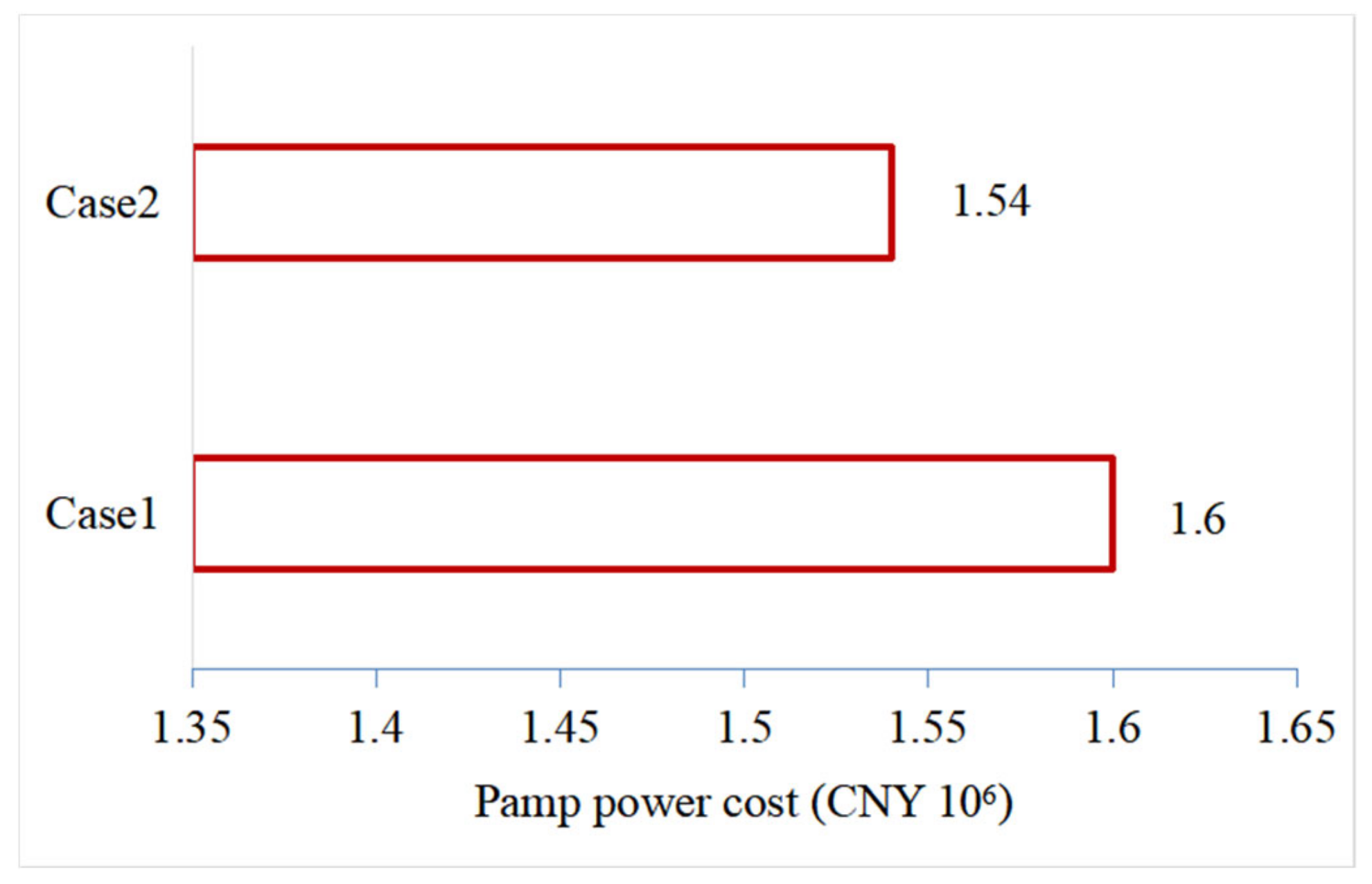
| Ramping power cost (CNY 107) | 1.60 | 1.54 | 3.75% |
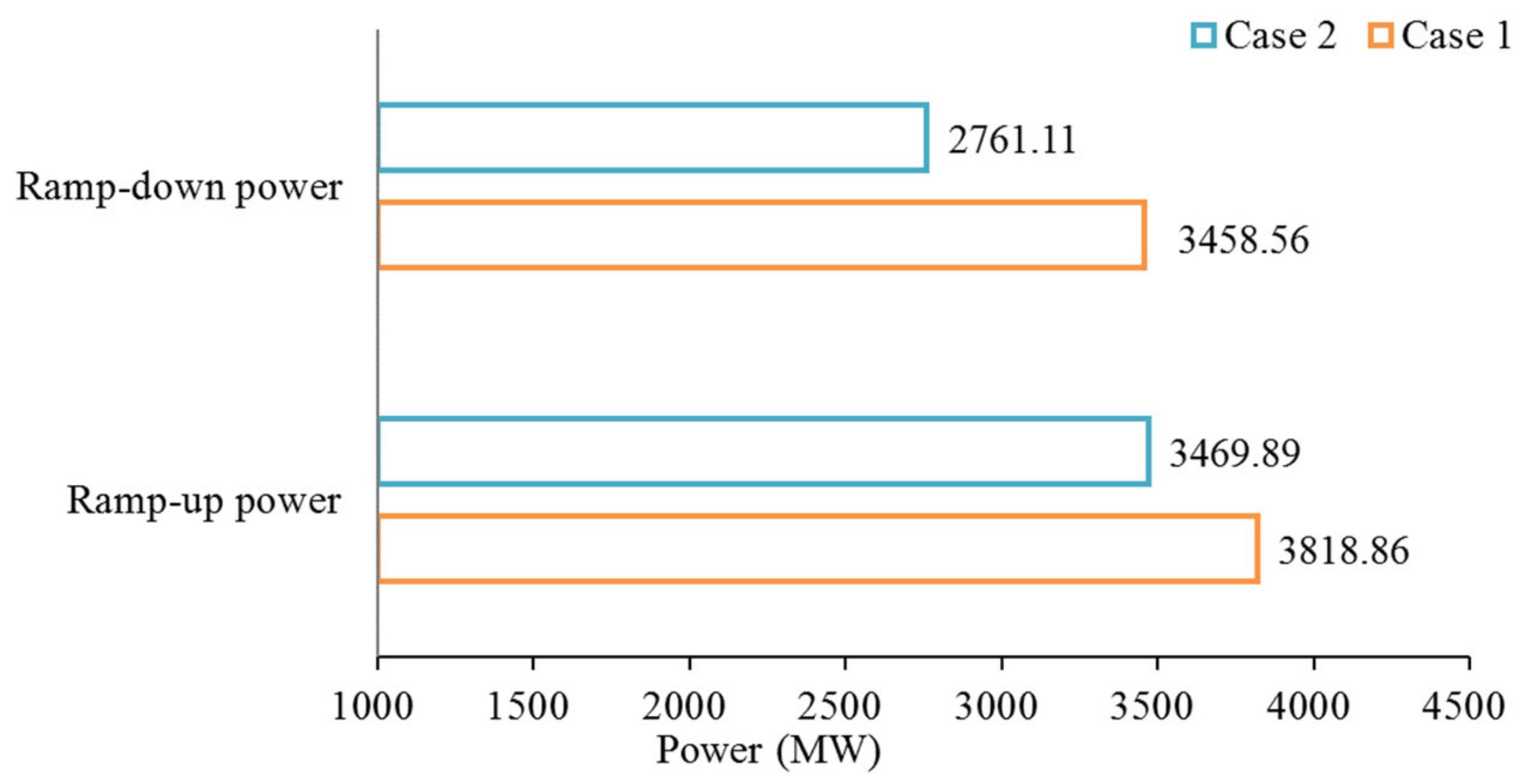
| Ramp-up power (MW) | 3818.86 | 3469.89 | 9.14% |
| Ramp-down power (MW) | 3458.56 | 2761.11 | 20.17% |
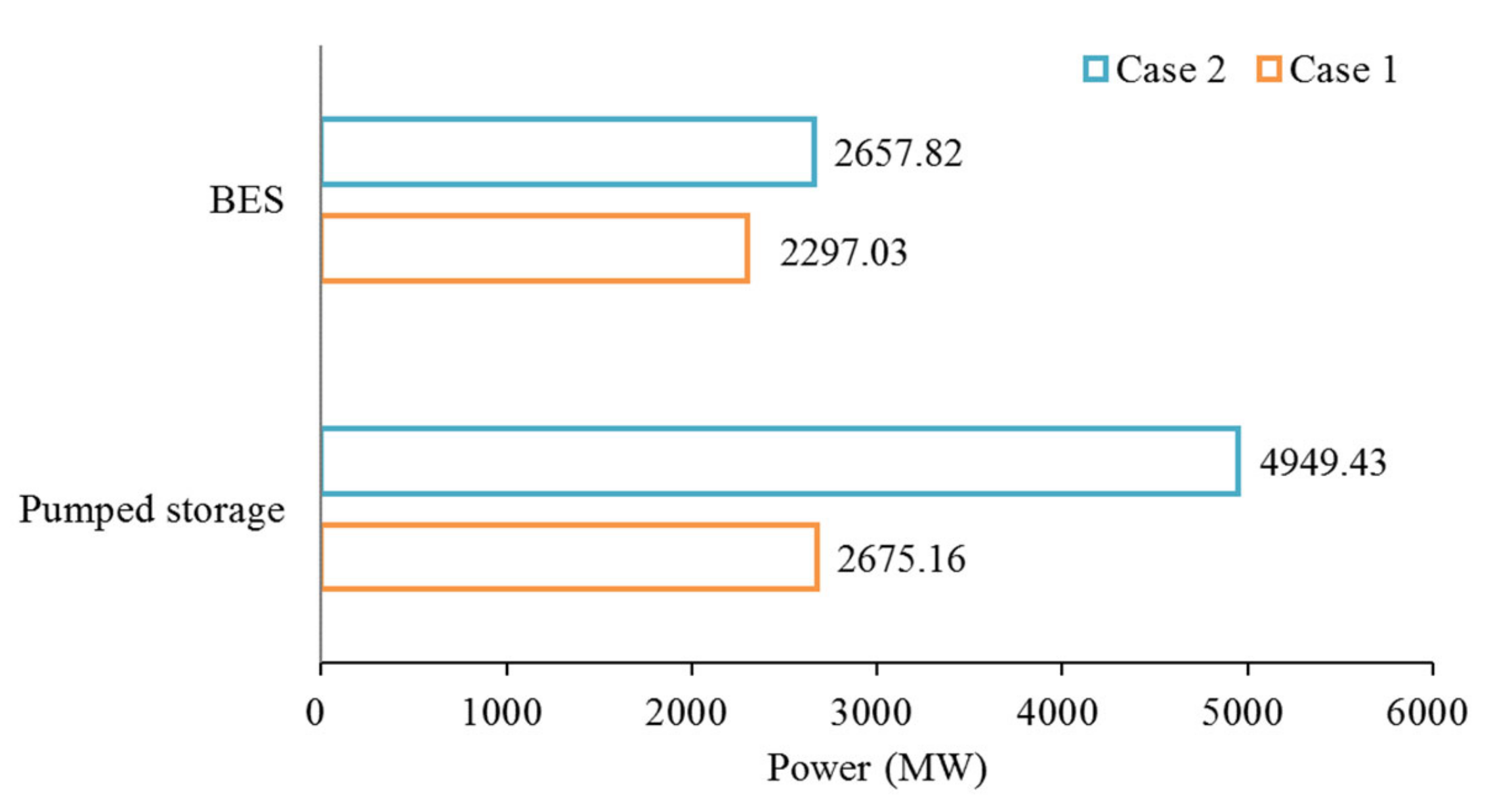
| Throughput of pumped storage (MW) | 2675.16 | 4949.43 | −85.01% |
| Throughput of BES (MW) | 2297.03 | 2657.82 | −15.71% |
| Case 3 | Case 4 | Decreasing Percentage in Case 3 | |
|---|---|---|---|
| Total operation cost (CNY 105) | 7.3702 | 7.3572 | 0.18% |
| Thermal operation cost (CNY 105) | 7.2060 | 7.2075 | −0.02% |
| Ramping power cost (CNY) | 11,920.06 | 10,225.84 | 16.57% |
| Ramp-up power (MW) | 1046.61 | 956.84 | 9.38% |
| Ramp-down power (MW) | 876.13 | 811.95 | 7.9% |
| Throughput of pumped storage (MW) | 938.94 | 1473.88 | −36.29% |
| Throughput of BES (MW) | 1381.42 | 1732.56 | −20.27% |
Publisher’s Note: MDPI stays neutral with regard to jurisdictional claims in published maps and institutional affiliations. |
© 2022 by the authors. Licensee MDPI, Basel, Switzerland. This article is an open access article distributed under the terms and conditions of the Creative Commons Attribution (CC BY) license (https://creativecommons.org/licenses/by/4.0/).
Share and Cite
Hu, S.; Gao, Z.; Wu, J.; Ge, Y.; Li, J.; Zhang, L.; Liu, J.; Sun, H. Time-Interval-Varying Optimal Power Dispatch Strategy Based on Net Load Time-Series Characteristics. Energies 2022, 15, 1582. https://doi.org/10.3390/en15041582
Hu S, Gao Z, Wu J, Ge Y, Li J, Zhang L, Liu J, Sun H. Time-Interval-Varying Optimal Power Dispatch Strategy Based on Net Load Time-Series Characteristics. Energies. 2022; 15(4):1582. https://doi.org/10.3390/en15041582
Chicago/Turabian StyleHu, Shubo, Zhengnan Gao, Jing Wu, Yangyang Ge, Jiajue Li, Lianyong Zhang, Jinsong Liu, and Hui Sun. 2022. "Time-Interval-Varying Optimal Power Dispatch Strategy Based on Net Load Time-Series Characteristics" Energies 15, no. 4: 1582. https://doi.org/10.3390/en15041582