Constant Phase Element in the Time Domain: The Problem of Initialization

Abstract

The constant phase element (CPE) is found in most battery and supercapacitor equivalent circuit models proposed to interpret data in the frequency domain. When these models are used in the time domain, the initial conditions in the fractional differential equations must be correctly imposed. The initial state problem remains controversial and has been analyzed by various authors in the last two decades. This article attempts to clarify this problem by proposing a procedure to prepare the initial state and defining a decay function that reveals the effect of the initial state in several illustrative examples. This decay function depends on the previous history, which is reflected in the time needed to prepare the initial state and on the current profile assumed for this purpose. This effect of the initial state is difficult to separate and can lead to the misinterpretation of the CPE parameter values.

1. Introduction

Fractional equivalent circuit models are widely used to represent the behavior of batteries and supercapacitors, both in the frequency and time domains [1,2,3,4,5], as they offer better accuracy with a lesser number of elements. These equivalent circuits include constant phase elements (CPEs), which are unequivocally observed in the experimental results obtained with electrochemical impedance spectroscopy (EIS) [6]. The phase of the impedance of a CPE is constant since it depends on the fractional exponent $\alpha$, but does not depend on the frequency, as shown in (1) [1,7]:

$$Z_{CPE}\left(j\omega \right)=\frac{1}{Q·{\left(j\omega \right)}^{\alpha }}=\frac{1}{Q{\omega }^{\alpha }}{e}^{-j\alpha \frac{\pi }{2}}$$

(1)

In addition, the phase is negative, so that this element is sometimes referred to as a fractional capacitor. The impedance of the CPE in the Laplace domain is:

$$Z_{CPE}\left(s\right)=\frac{1}{Q{s}^{\alpha }}.$$

(2)

There is interest in applying these models in the time domain [2,3,8,9,10] where the impedance (2) corresponds to a fractional derivative, as shown in (3), which is discussed in the next section.

$$i\left(t\right)=Q\frac{d^{\alpha }v\left(t\right)}{d{t}^{\alpha }}$$

(3)

To solve differential equations that include fractional derivatives, the initial conditions must be handled appropriately. However, the initial state problem remains controversial and has been discussed by various authors in the last two decades. Lorenzo and Hartley first recognized that a time-varying initialization is actually required for the fractional-order derivative [11]. Some other authors also indicated that initial histories rather than initial values at a point should be considered [12,13,14]. The term “aberration” has been introduced in relation to this phenomenon [15] and has been used by other authors [16]. One procedure to deal with this problem is to define an initialized operator, related to the history, to be imposed in the fractional derivative at the initial point [17,18]. An alternative proposal is the diffusive representation introduced by Sabatier [19] and the continuous-frequency-distributed model proposed by Trigeassou and Maamri [20], which were merged in the construction of a partial differential equation, where the initial state is a vector of infinite dimensions [20,21,22]. The equivalence and compatibility of the above two initialization theories have been demonstrated [18,23].

We focus the analysis of this work on a fractional element with impedance given by (2), with $0<\alpha <1$, which is the particular case of greatest interest in battery and supercapacitor models. One example of it corresponds to $\alpha =0.5$, which is often called Warburg impedance [24,25].

In this paper, we bring this problem to the attention of the battery and supercapacitor modeling community. Our main goal is to provide a detailed study of how the previous history, i.e., how the initial voltage -$v\left(0\right)$- is reached, affects the subsequent behavior of the system. To do this, we hypothesized that the initial voltage of a CPE with $0<\alpha <1$ may be written as $v\left(0\right)g\left(t\right)$, where $g\left(t\right)$ is a decay function between zero and one, with intermediate values and behavior between that of the resistor and that of the non-fractional capacitor. This decay function, closely related to the general initial function defined by other authors [17,18,26], is derived and analyzed for the CPE, ZARC (composed of the CPE in parallel with a resistor), and RC networks. In the paper, we also highlight the error tow which some definitions of the fractional derivative can lead.

A brief review of the basic definitions of fractional derivatives is provided in Section 2. Next, the decay function is calculated and discussed in Section 3 for a CPE, analyzing how the previous history of the CPE influences the time dependence of the function. The case of a ZARC element is discussed in Section 4, and the approximation of a CPE by a series RC network is considered in Section 5. Finally, a discussion of the results is presented in Section 6, and some conclusions and possible future work are provided in Section 7.

2. Fractional Derivatives

The most commonly used definitions of fractional derivatives start from the Riemann–Liouville fractional integral of order $\alpha$, given by [27]:

$${}_{0}I{}_t^{\alpha }f\left(t\right)={}_{0}D{}_t^{-\alpha }f\left(t\right)=\frac{1}{\mathsf{\Gamma }\left(\alpha \right)}{\int }_0^t\frac{f\left(\tau \right)}{{(t-\tau )}^{1-\alpha }}d\tau$$

(4)

where $\mathsf{\Gamma }\left(\alpha \right)$ is the Gamma function [27].

Using Definition (4), the Riemann–Liouville fractional derivative is defined as [27]:

$${}_0^{RL}D{}_t^{\alpha }f\left(t\right)={}_{0}D{}_t^m{}_{0}D{}_t^{\alpha -m}f\left(t\right),$$

(5)

with $m-1\le \alpha <m$, m a positive integer, so that:

$${}_0^{RL}D{}_t^{\alpha }f\left(t\right)=\frac{1}{\mathsf{\Gamma }(m-\alpha )}\frac{d^m}{d{t}^m}{\int }_0^t\frac{f\left(\tau \right)}{{(t-\tau )}^{1-m+\alpha }}d\tau .$$

(6)

Applying the Laplace transformation to (5), the following equation is obtained [27]:

$$\mathcal{L}\left[{}_0^{RL}D{}_t^{\alpha }f\left(t\right)\right]=s^{\alpha }\mathcal{L}\left[f\left(t\right)\right]-\sum _{k=0}^{m-1}{s}^k{\left[{}_0^{RL}D{}_t^{\alpha -k-1}f\left(t\right)\right]}_{t=0}$$

(7)

This expression depends on fractional derivatives at the initial time. This is a drawback of the Riemann–Liouville definition and motivates the use of an alternative definition known as the Caputo fractional derivative:

$${}_0^{C}D{}_t^{\alpha }f\left(t\right)={}_{0}D{}_t^{\alpha -m}{}_{0}D{}_t^{m}f\left(t\right),$$

(8)

or:

$${}_0^{C}D{}_t^{\alpha }f\left(t\right)=\frac{1}{\mathsf{\Gamma }(m-\alpha )}{\int }_0^t\frac{1}{{(t-\tau )}^{1-m+\alpha }}\frac{d^{m}f\left(\tau \right)}{d{\tau }^m}d\tau ,m-1\le \alpha <m,$$

(9)

whose Laplace transform is:

$$\mathcal{L}\left[{}_0^{C}D{}_t^{\alpha }f\left(t\right)\right]=s^{\alpha }\mathcal{L}\left[f\left(t\right)\right]-\sum _{k=0}^{m-1}{s}^{\alpha -k-1}{f}^{\left(k\right)}\left(0\right)$$

(10)

Equation (10) only uses integer derivatives at the initial time, so it is easier to apply in practice. However, the inability of the Caputo definition to provide a satisfactory solution to the initial condition problem has been pointed out [13,15], and we comment on it below.

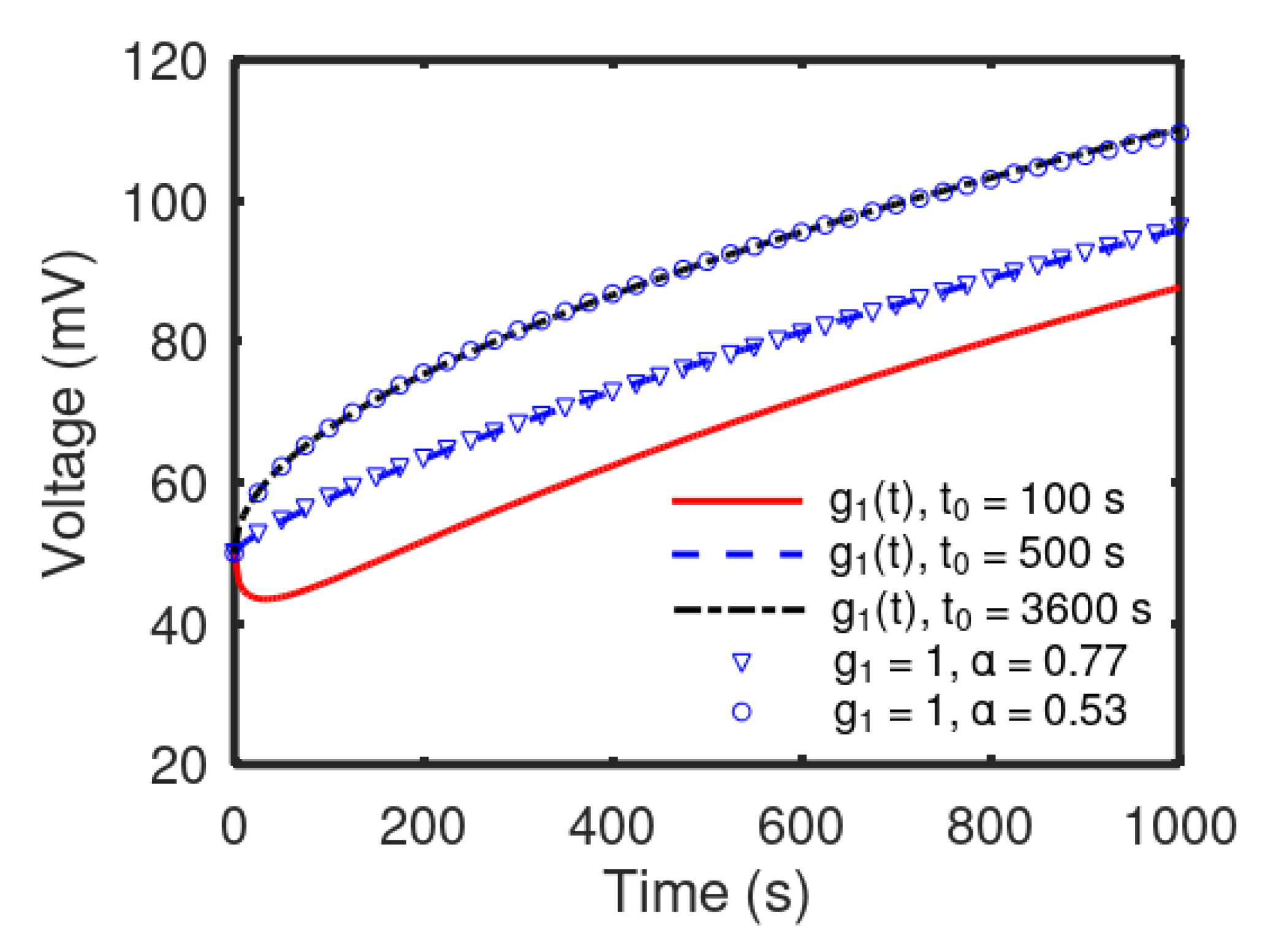
3. Initialization of the CPE

The CPE, or fractional capacitor, with $0<\alpha <1$, can be considered as an intermediate case between a resistor ($\alpha =0$) and an ideal non-fractional capacitor ($\alpha =1$). It is reasonable to think that it also behaves as an intermediate case in relation to the initial conditions. Allagui et al. [28] recently claimed that the weight of the voltage memory trace that results from the contribution of past voltage activity depends on the fractional exponent $\alpha$, and therefore, the measured response of the device at any time is increasingly correlated with its past, while ideal capacitors do not exhibit such behavior and are memoryless devices. We interpret this same result in another way. If this two-terminal element supports an initial voltage drop, $v\left(0\right)$, at time $t=0$, and we apply a current $i\left(t\right)$ for time $t>0$, the behavior in the two extreme cases is quite different. In the case of a resistor with resistance R, the voltage at time $t>0$ is:

$$v\left(t\right)=Ri\left(t\right),$$

(11)

and the initial voltage is immediately forgotten. In the opposite case of a non-fractional capacitor of capacitance C, the voltage is given by:

$$v\left(t\right)=v\left(0\right)+\frac{1}{C}{\int }_0^{t}i\left(\tau \right)d\tau ,$$

(12)

and the initial voltage is always remembered, although its later effects do not depend on the previous history.

Let us apply (10) to (3), in the particular case of $0<\alpha <1$, to obtain:

$$I\left(s\right)=Q\{s^{\alpha }V\left(s\right)-s^{\alpha -1}v\left(0\right)\},$$

(13)

or:

$$V\left(s\right)=\frac{I\left(s\right)}{Q{s}^{\alpha }}+\frac{v\left(0\right)}{s},$$

(14)

which in the time domain, for $t>0$, corresponds to:

$$v\left(t\right)=v\left(0\right)+\frac{1}{Q\mathsf{\Gamma }\left(\alpha \right)}{\int }_0^t\frac{i\left(\tau \right)}{{(t-\tau )}^{1-\alpha }}d\tau .$$

(15)

Time-domain models for predicting the voltage–current characteristics of lithiumion batteries under arbitrary charging and discharging current profiles have been reported, showing a higher accuracy than the traditional models with multiple parallel RC units [29,30]. The initial voltage has been considered in an equation similar to (14). With this way of initialization, $v\left(0\right)$ acts as an integration constant and is always remembered, as we would expect in the case of an ideal non-fractional capacitor, that it is not what we should obtain in the limit $\alpha \to 0$. Instead, we would expect to obtain:

$$v\left(t\right)=v\left(0\right)g\left(t\right)+\frac{1}{Q\mathsf{\Gamma }\left(\alpha \right)}{\int }_0^t\frac{i\left(\tau \right)}{{(t-\tau )}^{1-\alpha }}d\tau$$

(16)

so that the Caputo definition does not seem to produce the correct results. The meaning of $g\left(t\right)$ is discussed in the next section.

An alternative to the Riemann–Liouville and Caputo definitions of the fractional derivative is to use the discretized and truncated Grünwald–Letnikov derivative with a short and fixed memory length [5]. However, the voltage values during this memory interval, before the initial time, must also be known, so that the initialization problem is not solved by this approach.

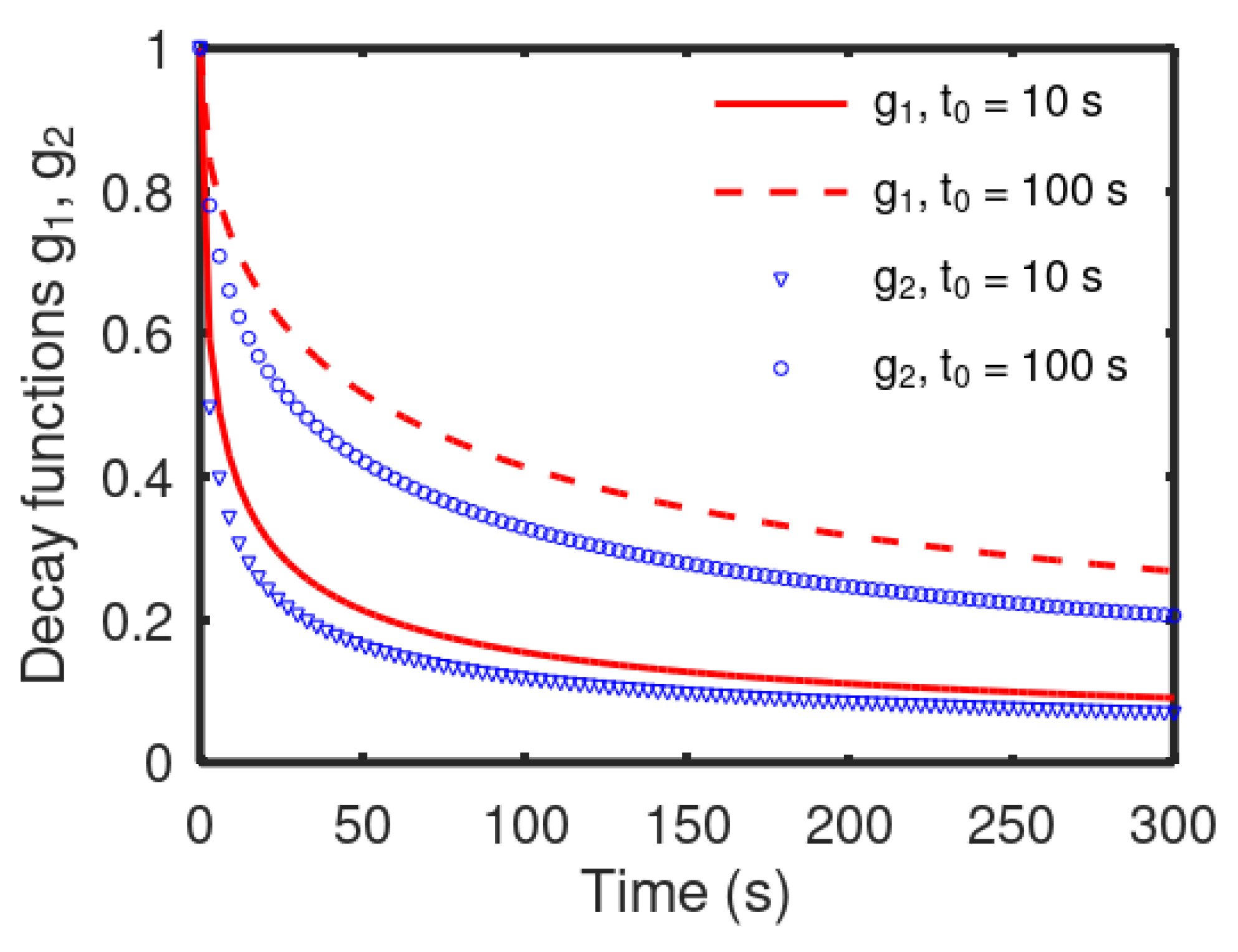
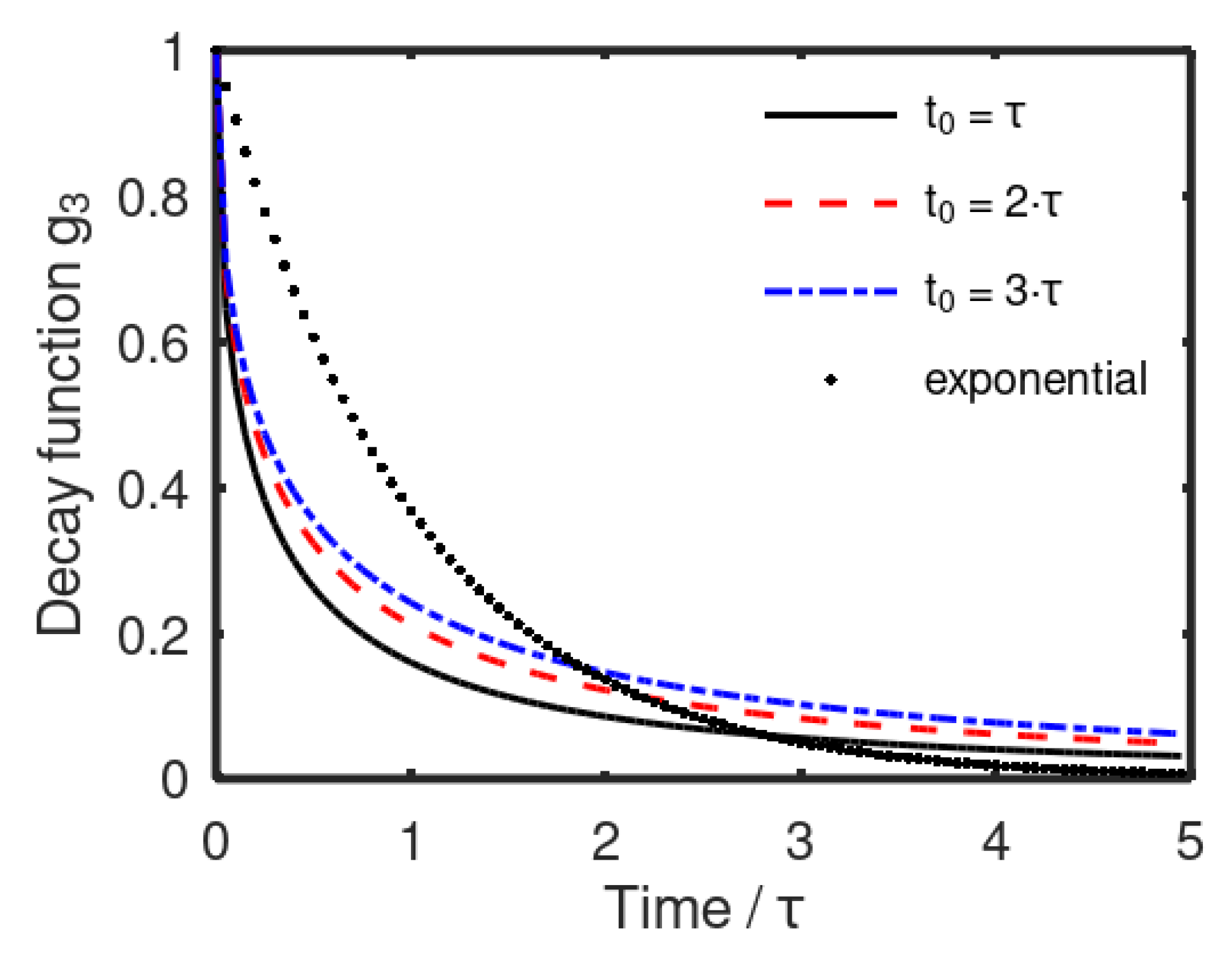
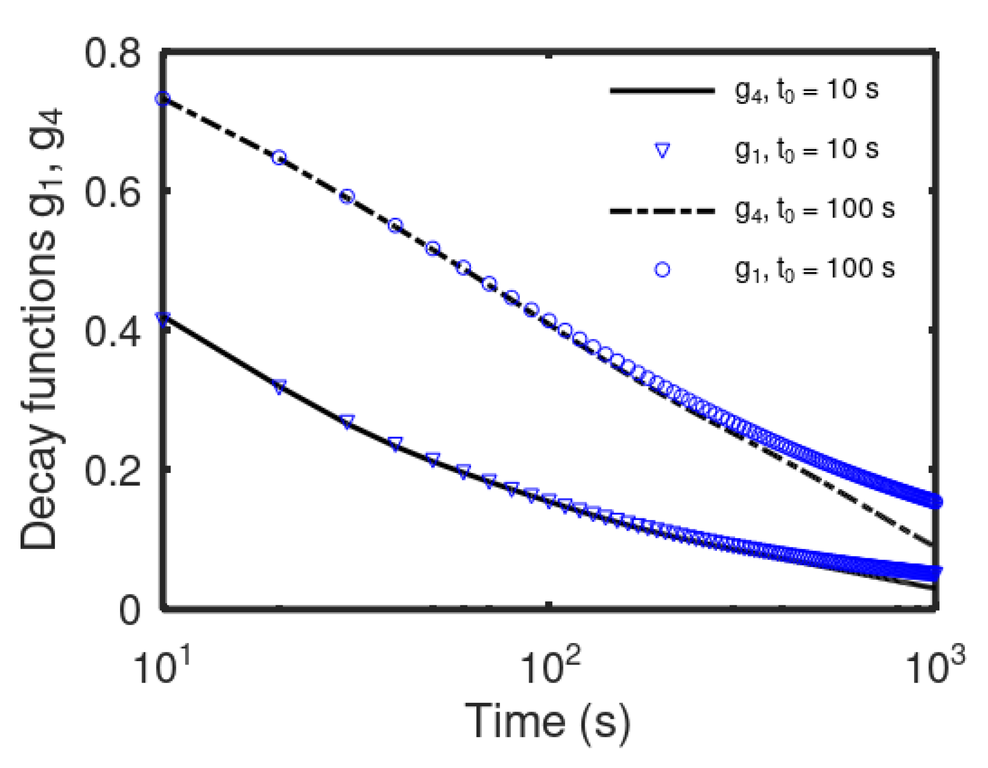
4. The Decay Function

To obtain the value of $g\left(t\right)$, which we call the decay function, we propose to prepare an initial state starting from a state with zero initial conditions. The idea of preparing an initial state is not actually new [19]. It was applied in [13] and [14] to compute the internal force of an axially loaded viscoelastic bar, where an initial state was defined over an interval, and the initial condition was called the initial history [13]. The initialization function is a time-varying function and can be viewed as a generalization of the constant of integration required for the order-one integral [31]. Zhao et al. [26] also applied this procedure to the case of the internal force of an axially loaded viscoelastic bar and showed that the influence caused by the pre-initial process varies in time and reflects the memory of the whole pre-initial process, which explains the origin of the long memory property of fractional-order systems [26].

We distinguish the initialization interval, $[0,t_0]$, and the observation interval, $(t_0,\infty )$, and assume that the initial state has been achieved at $t_0$ with an initialization current $i_0$ while the current applied during the observation phase is $i_1$, according to the next equation.

$$i\left(t\right)=\left\{\begin{array}{cc}{i}_0\left(t\right)\hfill & 0\le t<t_0\hfill \\ i_1\left(t-t_0\right)\hfill & t\ge t_0\hfill \end{array}\right.$$

(17)

We also assumed zero initial conditions prior to the initialization phase. With zero initial conditions, the two definitions of fractional derivative (6) and (9) lead to the same Laplace transform and the ambiguity is avoided.

To obtain the initial voltage $v_0$, we can apply a suitable constant current $i_0\left(t\right)=I_0$. With this current, the voltage can be obtained by:

$$v\left(t\right)=\frac{I_0}{Q\mathsf{\Gamma }\left(\alpha \right)}{\int }_0^t\frac{d\tau }{{(t-\tau )}^{1-\alpha }}=\frac{I_0{t}^{\alpha }}{Q\mathsf{\Gamma }(\alpha +1)},$$

(18)

If $I_0$ is held for a time interval of length $t_0$,

$$v\left(t_0\right)=\frac{I_0{t}_0^{\alpha }}{Q\mathsf{\Gamma }(\alpha +1)}\equiv v_0.$$

(19)

After $t_0$, an arbitrary current $i\left(t\right)$ flows through the CPE. The voltage is then obtained as:

$$v\left(t\right)=\frac{I_0}{Q\mathsf{\Gamma }\left(\alpha \right)}{\int }_0^{t_0}\frac{d\tau }{{(t-\tau )}^{1-\alpha }}+\frac{1}{Q\mathsf{\Gamma }\left(\alpha \right)}{\int }_{t_0}^t\frac{i\left(\tau \right)}{{(t-\tau )}^{1-\alpha }}d\tau .$$

(20)

The first term in (20) is:

$$\frac{I_0}{Q\mathsf{\Gamma }\left(\alpha \right)}{\int }_0^{t_0}\frac{d\tau }{{(t-\tau )}^{1-\alpha }}=\frac{I_0}{Q\mathsf{\Gamma }(\alpha +1)}[t^{\alpha }-{(t-t_0)}^{\alpha }],$$

(21)

which can be rewritten, by using (19), as:

$$\frac{I_0}{Q\mathsf{\Gamma }\left(\alpha \right)}{\int }_0^{t_0}\frac{d\tau }{{(t-\tau )}^{1-\alpha }}=v_0\left[{\left(\frac{t}{t_0}\right)}^{\alpha }-{\left(\frac{t-t_0}{t_0}\right)}^{\alpha }\right].$$

(22)

By defining the observation time, $t^{\prime }$, after $t_0$,

$$t^{\prime }\equiv t-t_0,$$

(23)

the final result has the form expected in (16):

$$\begin{array}{cc}\hfill v\left(t^{\prime }\right)& =v_0{g}_1(t_0;t^{\prime })+\frac{1}{Q\mathsf{\Gamma }\left(\alpha \right)}{\int }_0^{t^{\prime }}\frac{i(\tau +t_0)}{{(t^{\prime }-\tau )}^{1-\alpha }}d\tau \hfill \\ \hfill & =v_0{g}_1(t_0;t^{\prime })+\frac{1}{Q\mathsf{\Gamma }\left(\alpha \right)}{\int }_0^{t^{\prime }}\frac{i_1\left(\tau \right)}{{(t^{\prime }-\tau )}^{1-\alpha }}d\tau ,\hfill \end{array}$$

(24)

with:

$$g_1(t_0;t^{\prime })={\left(1+\frac{t^{\prime }}{t_0}\right)}^{\alpha }-{\left(\frac{t^{\prime }}{t_0}\right)}^{\alpha }.$$

(25)

Function $g_1$ verifies $g_1(t_0;0)=1$ and $li{m}_{t^{\prime }\to \infty }{g}_1(t_0;t^{\prime })=0$, so that the initial voltage, $v_0$, is eventually forgotten, which justified the name “decay function” we used for it. However, although this procedure gives a method to prepare an initial state, the function $g_1$ depends on the time $t_0$, which highlights the importance of taking into account the previous history since the same initial voltage can be obtained with different combinations of $I_0$ and $t_0$ values, and different decay rates of the initial voltage are therefore obtained.

The result also depends on the current profile used to prepare the initial state. To illustrate this, we can use a ramp current instead of a constant current for the same purpose. Let us assume a current $i_0\left(t\right)=a·t$ for $0\le t<t_0$. The voltage for this time interval is then:

$$v\left(t\right)=\frac{a}{Q\mathsf{\Gamma }\left(\alpha \right)}{\int }_0^t\frac{\tau ·d\tau }{{(t-\tau )}^{1-\alpha }}=\frac{a{t}^{\alpha +1}}{Q\mathsf{\Gamma }(\alpha +2)}$$

(26)

and:

$$v\left(t_0\right)=\frac{a{t}_0^{\alpha +1}}{Q\mathsf{\Gamma }(\alpha +2)}\equiv v_0.$$

(27)

If an arbitrary current $i\left(t\right)$ is applied after $t_0$,

$$v\left(t\right)=\frac{a}{Q\mathsf{\Gamma }\left(\alpha \right)}{\int }_0^{t_0}\frac{\tau d\tau }{{(t-\tau )}^{1-\alpha }}+\frac{1}{Q\mathsf{\Gamma }\left(\alpha \right)}{\int }_{t_0}^t\frac{i\left(\tau \right)}{{(t-\tau )}^{1-\alpha }}d\tau ,$$

(28)

where:

$$\frac{a}{Q\mathsf{\Gamma }\left(\alpha \right)}{\int }_0^{t_0}\frac{\tau d\tau }{{(t-\tau )}^{1-\alpha }}=\frac{a}{Q\mathsf{\Gamma }(\alpha +2)}[t^{\alpha +1}-{(t-t_0)}^{\alpha +1}-(\alpha +1)t_0{(t-t_0)}^{\alpha }].$$

(29)

Using (27),

$$\frac{a}{Q\mathsf{\Gamma }\left(\alpha \right)}{\int }_0^{t_0}\frac{\tau d\tau }{{(t-\tau )}^{1-\alpha }}=v_0\left[{\left(\frac{t}{t_0}\right)}^{\alpha +1}-{\left(\frac{t-t_0}{t_0}\right)}^{\alpha +1}-(\alpha +1){\left(\frac{t-t_0}{t_0}\right)}^{\alpha }\right]$$

(30)

With $t^{\prime }\equiv t-t_0$, the final result is obtained as:

$$v\left(t^{\prime }\right)=v_0{g}_2(t_0;t^{\prime })+\frac{1}{Q\mathsf{\Gamma }\left(\alpha \right)}{\int }_0^{t^{\prime }}\frac{i\left(\tau \right)}{{(t^{\prime }-\tau )}^{1-\alpha }}d\tau ,$$

(31)

where:

$$g_2(t_0;t^{\prime })={\left(1+\frac{t^{\prime }}{t_0}\right)}^{\alpha +1}-\left(1+\alpha +\frac{t^{\prime }}{t_0}\right){\left(\frac{t^{\prime }}{t_0}\right)}^{\alpha }$$

(32)

Again, $g_2(t_0;0)=1$ and $li{m}_{t^{\prime }\to \infty }{g}_2(t_0;t^{\prime })=0$, so that $g_2$ is another form of the decay function obtained for a different initialization current profile. The decay functions $g_1$ and $g_2$ are shown in Figure 1 for $\alpha =0.5$ and two different values of $t_0$. The decay rates are slow for long times and are different in the four cases, thus proving the influence of the previous history.

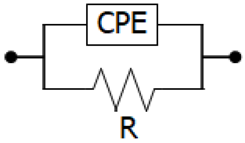
5. Initialization of ZARC

The CPE included in battery and supercapacitor models is often connected with a resistor in parallel, as shown in Figure 2. For this connection, the name ZARC was proposed earlier [32] and has been widely used ever since [1,2,10]. Its impedance in the Laplace domain is:

$$Z=\frac{R}{1+RQ{s}^{\alpha }}$$

(33)

Instead of parameter Q, we can use a time constant, which can be used as a time reference, by defining $\tau \equiv {\left(RQ\right)}^{\frac{1}{\alpha }}$, so that:

$$Z=\frac{R}{1+{\left(\tau s\right)}^{\alpha }}$$

(34)

and:

$$\left[1+{\left(\tau s\right)}^{\alpha }\right]V\left(s\right)=I\left(s\right)R.$$

(35)

We apply now the same initialization procedure used above with a constant current, $I_0$, to prepare the initial state. An arbitrary current $i_1$ is subsequently applied for $t\ge t_0$:

$$i\left(t\right)=\left\{\begin{array}{cc}{I}_0\hfill & 0\le t<t_0\hfill \\ i_1\left(t-t_0\right)\hfill & t\ge t_0\hfill \end{array}\right.$$

(36)

Equation (36) can be rewritten as:

$$i\left(t\right)=I_0[u\left(t\right)-u(t-t_0)]+i_1(t-t_0)u(t-t_0),$$

(37)

where $u\left(t\right)$ is the unit step function. Its Laplace transform is [29]:

$$I\left(s\right)=I_0\frac{1-e^{-s{t}_0}}{s}+I_1\left(s\right)e^{-s{t}_0}.$$

(38)

so that:

$$V\left(s\right)=I_{0}R\frac{1-e^{-s{t}_0}}{s\left[1+{\left(\tau s\right)}^{\alpha }\right]}+I_1\left(s\right)R\frac{e^{-s{t}_0}}{1+{\left(\tau s\right)}^{\alpha }}.$$

(39)

For $t\ge t_0$, or $t^{\prime }\ge 0$, where $t^{\prime }=t-t_0$, we obtain:

$$v\left(t^{\prime }\right)=v_{ini}(t_0;t^{\prime })+v_1\left(t^{\prime }\right)$$

(40)

where:

$$v_1\left(t^{\prime }\right)={\mathcal{L}}^{-1}\left[\frac{I_1\left(s\right)R}{1+{\left(\tau s\right)}^{\alpha }}\right]$$

(41)

is the voltage that we would obtain in response to $i_1$ with zero initial conditions, and:

$$v_{ini}(t_0;t^{\prime })={\mathcal{L}}^{-1}\left[\frac{I_{0}R(1-e^{-s{t}_0})}{s\left[1+{\left(\tau s\right)}^{\alpha }\right]}\right].$$

(42)

is the response to the initial voltage in the observation phase. By using [27]:

$${\mathcal{L}}^{-1}\left[\frac{1}{s\left[1+{\left(\tau s\right)}^{\alpha }\right]}\right]=1-E_{\alpha }\left[-{\left(\frac{t}{\tau }\right)}^{\alpha }\right]$$

(43)

where $E_{\alpha }\left(x\right)$ is the one-parameter Mittag–Leffler function [27], defined according to:

$$E_{\alpha }\left(x\right)=\sum _{n=0}^{\infty }\frac{x^n}{\mathsf{\Gamma }(n\alpha +1)}$$

(44)

the result, with $t^{\prime }=t-t_0$, is:

$$v_{ini}(t_0;t^{\prime })=I_{0}R\left\{\left[1-E_{\alpha }\left(-{\left(\frac{t^{\prime }+t_0}{\tau }\right)}^{\alpha }\right)\right]-\left[1-E_{\alpha }\left(-{\left(\frac{t^{\prime }}{\tau }\right)}^{\alpha }\right)\right]\right\}$$

(45)

The initial voltage can be written as:

$$v_0\equiv v_{ini}(t_0;0)=I_{0}R\left[1-E_{\alpha }\left(-{\left(\frac{t_0}{\tau }\right)}^{\alpha }\right)\right],$$

(46)

so that the final result is:

$$v_{ini}(t_0;t^{\prime })=v_0{g}_3(t_0;t^{\prime }),$$

(47)

where a new decay function $g_3$ is defined in this case according to:

$$g_3(t_0;t^{\prime })=\frac{E_{\alpha }\left(-{\left(\frac{t^{\prime }}{\tau }\right)}^{\alpha }\right)-E_{\alpha }\left(-{\left(\frac{t^{\prime }+t_0}{\tau }\right)}^{\alpha }\right)}{1-E_{\alpha }\left(-{\left(\frac{t_0}{\tau }\right)}^{\alpha }\right)}.$$

(48)

In the case of a non-fractional ZARC, which is obtained in the limit $\alpha =1$, in which the CPE is substituted by a non-fractional capacitor, and taking into account that the Mittag–Leffler function reduces to the exponential function in this limit:

$$\underset{\alpha \to 1}{lim}{E}_{\alpha }\left[-{\left(\frac{t^{\prime }}{\tau }\right)}^{\alpha }\right]=e^{-\left(\frac{t^{\prime }}{\tau }\right)},$$

(49)

and the decay function is also an exponential function:

$$\underset{\alpha \to 1}{lim}{g}_3(t_0;t^{\prime })=e^{-\left(\frac{t^{\prime }}{\tau }\right)}.$$

(50)

This is the well-known result in the case of the parallel RC network, in which the effect of the initial voltage decays exponentially.

Therefore, both in the fractional ZARC and in the parallel RC network, the effect of the initial voltage decays and eventually vanishes, but while in the case of the parallel RC network, the exponential decay only depends on the initial voltage, in the case of the fractional ZARC, the decay rate is smoother and depends on the previous history. This behavior is compared in Figure 3, for the case of $\alpha =0.5$. The decay function $g_3$ decays rapidly at first, but the decay rate is quite slower than the exponential for long times.

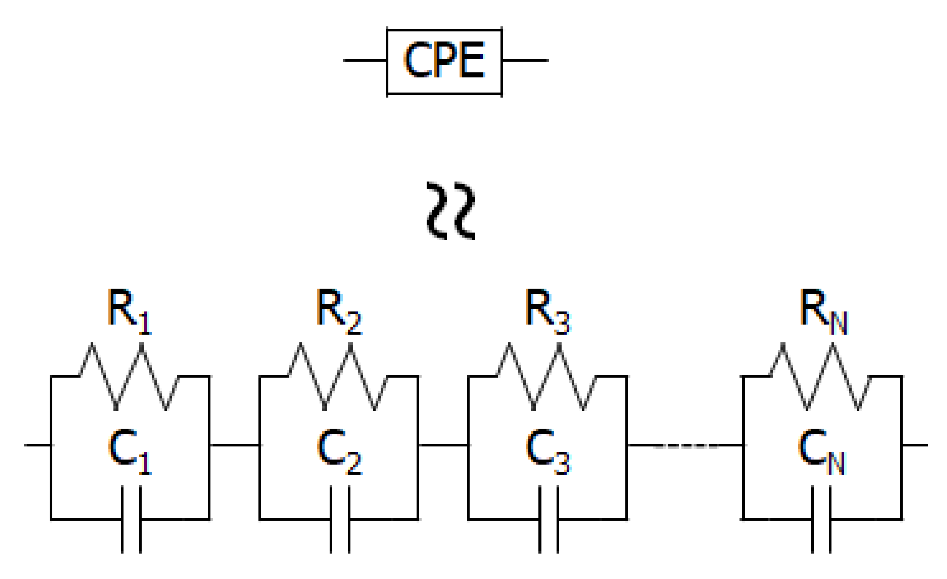
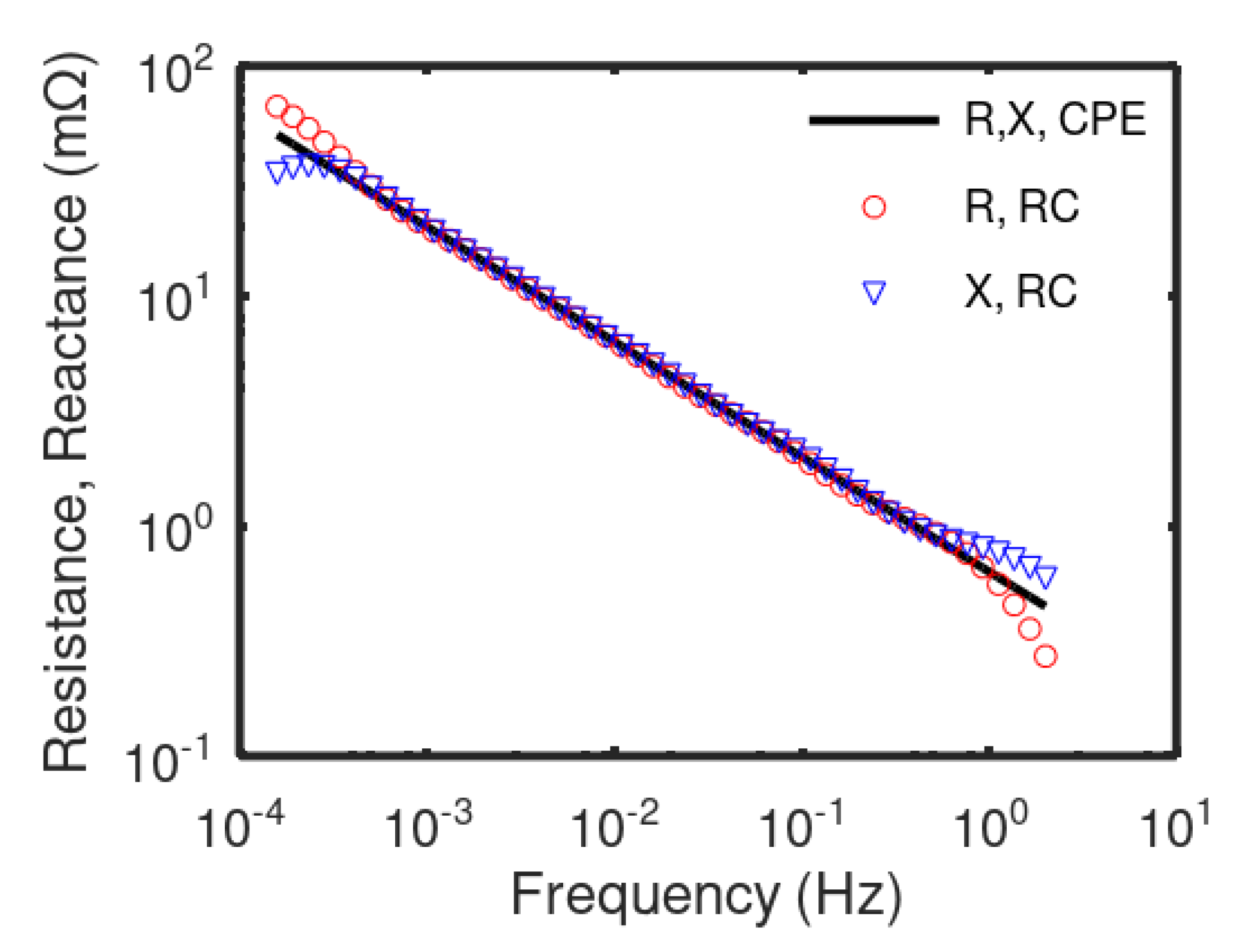
6. Approximation of the CPR by an RC Network

To avoid the problems associated with the fractional derivatives, the fractional impedances are often approximated by functions with a finite number of poles and zeros. One possibility is that proposed by [33], and used by other authors [8], in which the fractional-order transfer function is approximated with a high-degree integer-order system. Another option is to approximate the CPE (or the ZARC) by a network composed by a series of RC branches [6,34], as shown in Figure 4. The approximation of the ZARC using finite and infinitely serially connected RC circuits was analyzed in detail in [35]. We consider the approximation of a CPE by a series RC network in this section.

We could think that by using non-fractional RC elements, in which the effect of the initial voltage does not depend on the previous history, the problem of the initial conditions that we discussed above can be avoided. However, this is not true, since given an initial voltage $v_0$ in the network, how this voltage is distributed among the initial voltages of the different elements actually depends on the previous history.

The voltage of the RC network, with N parallel RC elements connected in series, can be obtained as follows [24],

$$v\left(t\right)=v_{0}g\left(t\right)+\sum _{n=1}^N\frac{1}{C_n}{\int }_0^{t}i\left(\xi \right)e^{-\frac{t-\xi }{{\tau }_n}}d\xi ,$$

(51)

with:

$$g\left(t\right)=\frac{{\sum }_{n=1}^N{v}_{n,0}{e}^{-\frac{t}{{\tau }_n}}}{{\sum }_{n=1}^N{v}_{n,0}},$$

(52)

where $v_{n,0}$ is the initial voltage in the n-th element, and:

$$v_0=\sum _{n=1}^N{v}_{n,0}$$

(53)

We prepare the initial state again by starting from the zero initial condition and applying a constant current, $I_0$, for a time $t_0$. The initial voltage in the n-th element in the observation phase, at the end of this period, is obtained as:

$$v_{n,0}=I_0{R}_n\left(1-e^{-\frac{t_0}{{\tau }_n}}\right)$$

(54)

and the decay function is also obtained in this case:

$$g\left(t\right)=g_4(t_0;t)=\frac{{\sum }_{n=1}^N{R}_n\left(1-e^{-\frac{t_0}{{\tau }_n}}\right)e^{-\frac{t}{{\tau }_n}}}{{\sum }_{n=1}^N{R}_n\left(1-e^{-\frac{t_0}{{\tau }_n}}\right)},$$

(55)

where time t is measured after the initialization period. The new decay function also has the expected limits $li{m}_{t\to \infty }{g}_4(t_0;t)=0$ and $li{m}_{t\to 0}{g}_4(t_0;t)=1$.

The behavior of the decay function $g_4$ can be compared with the decay function $g_1$ of the CPE that the RC network approximates. To do so, we considered a Warburg-type CPE, with $\alpha =0.5$, and approximated it by an RC network with five elements ($N=5$). We used typical parameter values of a Warburg impedance for a Li-ion battery [8,34]: (1) The values of $R_n$ and ${\tau }_n=R_n{C}_n$ were obtained by a least-square fit to the real and imaginary parts of the CPE impedance in the range $f_{min}=1$ MHz to $f_{max}\simeq 1$ Hz. (2) The real part of the CPE impedance at 1 MHz is 20 m$\mathsf{\Omega }$. The values of the RC network components are provided in

Table 1. Values of the parameters for the RC elements.

n	1	2	3	4	5
$R_n$ (m$\mathsf{\Omega }$)	1.0407	1.9991	4.5240	10.5239	71.3679
${\tau }_n$ (s)	0.1352	1.8012	12.3951	70.7794	686.9286

.

Figure 5 shows a comparison of the real and imaginary parts of the impedances of the CPE (solid line) and the RC network (symbols). Since we chose $\alpha =0.5$, the real and imaginary parts of the CPE match. A good fit was obtained within the frequency range used for the adjustment, but deviations were observed outside this range. The two decay functions $g_1$ and $g_4$, given in (25) and (55), respectively, are compared in Figure 6 in logarithmic scales for two different values of $t_0$. A good agreement was observed for times less than $t_{max}\simeq \frac{1}{2\pi f_{min}}$, but a deviation was produced for longer times, in which the initial voltage for the CPE decayed at a lower rate.

7. Discussion

Although the problem of the initialization of fractional differential equations has been studied in the last two decades, it has not received sufficient consideration in some practical applications. The case considered here is the use of constant-phase elements in battery and supercapacitor modeling. When equivalent circuits containing fractional elements are used to predict the evolution of voltage and current in the time domain, the correct treatment of the initial conditions poses considerable difficulties, since many times, the previous history is not well known and its influence has been clearly demonstrated. The response to an applied current has been shown to be superimposed on the initial voltage multiplied by a decay function that depends on the previous current profile and the time for which it has been applied. There are several possibilities. The simplest one is to be sure that we start from a state with zero initial conditions, but this requires long relaxation times and is not always applicable. Another option is to wait for a long period after which the effect of the initial conditions has decayed and has a negligible effect on the element voltage, but this is even more difficult with fractional elements since the decay rates can be quite slow. A third possibility is to try to adjust the decay function from the data actually measured by separating it from the response to the post-initial current. Du et al. mentioned the difficulties of obtaining the initialization function in practical situations [15], although an algorithm to accomplish this task has been recently proposed [36]. In fact, this is not an easy task, as we show in the example below.

Let us prepare an initial voltage of 50 mV in a CPE of the Warburg type according to (1) with $\alpha =0.5$ and $Q=446{\mathsf{\Omega }}^{-1}$s${}^{\frac{1}{2}}$ (such that its real part is 20 m$\mathsf{\Omega }$ for a frequency of 1 MHz). We then apply a constant current $I_1=1$ A. Measuring the time t after the initialization period and using (24) we find:

$$v\left(t\right)=v_0{g}_1(t_0;t)+\frac{I_1{t}^{\alpha }}{Q\mathsf{\Gamma }(\alpha +1)},$$

(56)

where function $g_1$ is given in (25). The result, for three different values of $t_0$, namely 100 s, 500 s, and 3600 s, respectively, is shown in Figure 7. The curve corresponding to $t_0=100$ s initially decreases and then shows a turnaround behavior. This is a consequence of a high current in the initialization phase, since to obtain the initial value of 50 mV in $t_0=100$ s, a high initialization current, $I_0=1.98$ A, is needed. If the CPE is assumed to reflect, for example, a diffusion mechanism in a Li-ion battery [37], such a high current would have produced a highly nonuniform Li concentration in its particles [38], and the observed rebound is justified. However, in the other two cases, it is possible to misinterpret the data by assuming the wrong Equation (15) that corresponds to (56) with $g_1=1$ and different values of Q and $\alpha$. A good fit, shown with symbols in Figure 7, was obtained with $\alpha =0.77$ and $Q=4730$ ${\mathsf{\Omega }}^{-1}$s${}^{\alpha }$ for the $t_0=500$ s case and $\alpha =0.53$ and $Q=718$ ${\mathsf{\Omega }}^{-1}$s${}^{\alpha }$ for the $t_0=3600$ s case, different from those used in (56). In the slower initialization case ($I_0=0.33$ A during 3600 s), the error in Q and $\alpha$ is lower, but still important. The good fit obtained in some cases, such as those considered here with $t_0$ equal to 500 s and 3600 s, justifies the good result obtained by the authors, who used a non-decaying initial voltage [29,30]. However, the CPE parameter values obtained to represent the experimental results would have been different if a suitable decay function had been included. In other cases, such as the one shown here for $t_0=100$ s, it would have been much more difficult to obtain a good fit to the experimental results.

8. Conclusions and Future Research

To conclude, careful attention should be paid to the initialization of fractional elements, such as the CPE, in battery and supercapacitor models. The effect of the initial value decays with time and eventually vanishes, and it can be written as an initial function obtained as the product of the initial value and a decay function, but the initial function may be very difficult to separate from the rest of the response and may be misinterpreted by different values of the CPE parameters.

In many practical cases, the initial voltage can be measured or deduced if the open circuit voltage of the battery cell is known, but the previous history is usually not known, so it is not possible to obtain an accurate initialization function. However, in cases where the experiment cannot be designed starting from zero initial conditions, the decay functions proposed in this work can be used with an equivalent or effective $t_0$ parameter. This might not be totally accurate, but it would lead to better results than simply assuming an initial voltage that does not decay. We believe that this subject warrants further research. In those experimental works that seek to adjust the transient experimental results in the time domain with models that include the CPE, in addition to the CPE parameters, a new parameter defining the decay function can be included, and its effects on the accuracy or theoretical validity of the obtained results can be analyzed.

References

1. Andre, D.; Meiler, M.; Steiner, K.; Walz, H.; Soczka-Guth, T.; Sauer, D.U. A retrospective on lithium-ion batteries. J. Power Sources 2011, 196, 5349–5356. [Google Scholar] [CrossRef]
2. Wang, B.; Li, S.E.; Peng, H.; Liu, Z. Fractional-order modeling and parameter identification for lithium-ion batteries. J. Power Sources 2015, 293, 151–161. [Google Scholar] [CrossRef]
3. Bertrand, N.; Sabatier, J.; Briat, O.; Vinassa, J.M. Embedded Fractional Nonlinear Supercapacitor Model and Its Parametric Estimation Method. IEEE Trans. Ind. Electron. 2010, 57, 3991–4000. [Google Scholar] [CrossRef]
4. Allagui, A.; Freeborn, T.J.; Elwakil, A.S.; Maundy, B.J. Reevaluation of Performance of Electric Double-layer Capacitors from Constant-current Charge/Discharge and Cyclic Voltammetry. Sci. Rep. 2016, 6, 38568. [Google Scholar] [CrossRef] [PubMed]
5. Hu, X.; Yuan, H.; Zou, C.; Li, Z.; Zhang, L. Co-Estimation of State of Charge and State of Health for Lithium-Ion Batteries Based on Fractional-Order Calculus. IEEE Trans. Veh. Technol. 2018, 67, 10319–10329. [Google Scholar] [CrossRef]
6. Gagneur, L.; Driemeyer-Franco, A.; Forgez, C.; Friedrich, G. Modeling of the diffusion phenomenon in a lithium-ion cell using frequency or time domain identification. Microelectron. Reliab. 2013, 53, 784–796. [Google Scholar] [CrossRef]
7. Fouda, M.E.; Allagui, A.; Elwakil, A.S.; Das, S.; Psychalinos, C.; Radwan, A.G. Nonlinear charge-voltage relationship in constant phase element. AEU Int. J. Electron. Commun. 2020, 117, 153104. [Google Scholar] [CrossRef]
8. Alavi, S.M.M.; Birkl, C.R.; Howey, D.A. Time-domain fitting of battery electrochemical impedance models. J. Power Sources 2015, 288, 345–352. [Google Scholar] [CrossRef]
9. Allagui, A.; Freeborn, T.J.; Elwakil, A.S.; Fouda, M.E.; Maundy, B.J.; Radwan, A.G.; Said, Z.; Abdelkareem, M.A. Review of fractional-order electrical characterization of supercapacitors. J. Power Sources 2018, 400, 457–467. [Google Scholar] [CrossRef]
10. Nasser-Eddine, A.; Huard, B.; Gabano, J.D.; Poinot, T. A two steps method for electrochemical impedance modeling using fractional order system in time and frequency domains. Control Eng. Pract. 2019, 86, 96–104. [Google Scholar] [CrossRef]
11. Hartley, T.T.; Lorenzo, C. Dynamics and Control of Initialized Fractional-Order Systems. Nonlinear Dyn. 2002, 29, 201–233. [Google Scholar] [CrossRef]
12. Fukunaga, M.; Shimizu, N. Role of prehistories in the initial value problems of fractional viscoelastic equations. Nonlinear Dyn. 2004, 38, 207–220. [Google Scholar] [CrossRef]
13. Du, M.L.; Wang, Z.H. Initialized fractional differential equations with Riemann–Liouville fractional-order derivative. Eur. Phys. J. Spec. Top. 2011, 193, 49–60. [Google Scholar] [CrossRef]
14. Du, B.; Wei, Y.; Liang, S.; Wang, Y. Estimation of exact initial states of fractional order systems. Nonlinear Dyn. 2016, 86, 2061–2070. [Google Scholar] [CrossRef]
15. Du, M.; Wang, Z. Correcting the initialization of models with fractional derivatives via history-dependent conditions. Acta Mech. Sin. 2016, 32, 320–325. [Google Scholar] [CrossRef]
16. Zhao, Y.; Wei, Y.; Chen, Y.; Wang, Y. A new look at the fractional initial value problem: The aberration phenomenon. J. Comput. Nonlinear Dyn. 2018, 13, 121004. [Google Scholar] [CrossRef]
17. Lorenzo, C.F.; Hartley, T. Initialization of fractional-order operators and fractional differential equations. J. Comput. Nonlinear Dyn. 2008, 3, 021101. [Google Scholar] [CrossRef]
18. Hartley, T.T.; Lorenzo, C.F.; Trigeassou, J.C.; Maamri, N. Equivalence of history-function based and infinite-dimensional-state initializations for fractional-order operators. J. Comput. Nonlinear Dyn. 2013, 8, 041014. [Google Scholar] [CrossRef]
19. Sabatier, J.; Merveillaut, M.; Malti, R.; Oustaloup, A. How to impose physically coherent initial conditions to a fractional system? Commun. Nonlinear Sci. Numer. Simul. 2010, 15, 1318–1326. [Google Scholar] [CrossRef]
20. Trigeassou, J.C.; Maamri, N. Initial conditions and initialization of linear fractional differential equations. Signal Process. 2011, 91, 427–436. [Google Scholar] [CrossRef]
21. Trigeassou, J.C.; Maamri, N.; Sabatier, J.; Oustaloup, A. State variables and transients of fractional order differential systems. Comput. Math. Appl. 2012, 64, 3117–3140. [Google Scholar] [CrossRef] [Green Version]
22. Trigeassou, J.; Maamri, N.; Oustaloup, A. Lyapunov stability of noncommensurate fractional order systems: An energy balance approach. J. Comput. Nonlinear Dyn. 2016, 11, 041007. [Google Scholar] [CrossRef]
23. Yuan, J.; Zhang, Y.; Liu, J.; Shi, B. Equivalence of initialized fractional integrals and the diffusive model. J. Comput. Nonlinear Dyn. 2018, 13, 034501. [Google Scholar] [CrossRef]
24. Plett, G.L. Battery Management Systems, Volume I: Battery Modeling; Artech House: Noewood, MA, USA, 2015. [Google Scholar]
25. Agudelo, B.O.; Zamboni, W.; Monmasson, E. A Comparison of Time-Domain Implementation Methods for Fractional-Order Battery Impedance Models. Energies 2021, 14, 4415. [Google Scholar] [CrossRef]
26. Zhao, Y.; Wei, Y.; Shuai, J.; Wang, Y. Fitting of the initialization function of fractional order systems. Nonlinear Dyn. 2018, 93, 1589–1598. [Google Scholar] [CrossRef]
27. Petras, I. Fractional-Order Nonlinear Systems. Modeling, Analysis and Simulation; Springer: Berlin/Heidelberg, Germany, 2011. [Google Scholar]
28. Allagui, A.; Zhang, D.; Khakpour, I.; Elwakil, A.S.; Wang, C. Quantification of memory in fractional-order capacitors. J. Phys. D Appl. Phys. 2020, 53, 02LT03. [Google Scholar] [CrossRef]
29. Cheng, C.S.; Chung, H.S.H.; Lau, R.W.H. Time-domain modeling of constant phase element for simulation of lithium batteries under arbitrary charging and discharging current profiles. In Proceedings of the 2017 IEEE Applied Power Electronics Conference and Exposition (APEC), Tampa, FL, USA, 26–30 March 2017; pp. 985–992. [Google Scholar] [CrossRef]
30. Cheng, C.S.; Chung, H.S.H.; Lau, R.W.H.; Hong, K.Y.W. Time-Domain Modeling of Constant Phase Elements for Simulation of Lithium Battery Behavior. IEEE Trans. Power Electron. 2019, 34, 7573–7587. [Google Scholar] [CrossRef]
31. Yuan, J.; Gao, S.; Xiu, G.; Shi, B. Equivalence of initialized Riemann–Liouville and Caputo derivatives. J. Appl. Anal. Comput. 2020, 10, 2008–2023. [Google Scholar] [CrossRef]
32. Macdonald, J.R. New aspects of some small-signal ac frequency response functions. Solid State Ion. 1985, 15, 159–161. [Google Scholar] [CrossRef]
33. Oustaloup, A.; Levron, F.; Mathieu, B.; Nanot, F. Frequency-band complex noninteger differentiator: Characterization and synthesis. IEEE Trans. Circuits Syst. I Fundam. Theory Appl. 2000, 47, 25–30. [Google Scholar] [CrossRef]
34. Ren, H.; Zhao, Y.; Chen, S.; Yang, L.A. A comparative study of lumped equivalent circuit models of a lithium battery for state of charge prediction. Int. J. Energy Res. 2019, 43, 7306–7315. [Google Scholar] [CrossRef]
35. Heil, T.; Hossen, A. Continuous approximation of the ZARC element with passive components. Meas. Sci. Technol. 2021, 32, 104011. [Google Scholar] [CrossRef]
36. Krishnan, G.; Das, S.; Agarwal, V. An Online Identification Algorithm to Determine the Parameters of the Fractional-Order Model of a Supercapacitor. IEEE Trans. Ind. Appl. 2020, 56, 763–770. [Google Scholar] [CrossRef]
37. Nasser-Eddine, A.; Huard, B.; Gabano, J.D.; Poinot, T.; Martemianov, S.; Thomas, A. Fast time domain identification of electrochemical systems at low frequencies using fractional modeling. J. Electroanal. Chem. 2020, 862, 113957. [Google Scholar] [CrossRef]
38. Lopez-Villanueva, J.A.; Rodriguez-Bolivar, S.; Parrilla, L.; Finana, C. Simple Single Particle Model for Interpreting Fast Charge Results in Intercalation Batteries. In Proceedings of the XXXV Conference on Design of Circuits and Integrated Systems (DCIS), Segovia, Spain, 18–20 November 2020; pp. 1–5. [Google Scholar] [CrossRef]
Figure 1. Decay functions of the initial voltage obtained for a CPE with α = 0.5 by applying a constant current (lines) or a ramp current (symbols) for a time t 0 .
Energies 15 00792 g001
Figure 2. ZARC composed by a resistor and a CPE connected in parallel.
Energies 15 00792 g002
Figure 3. Decay function of the initial voltage obtained for a ZARC with α = 0.5 by applying a constant current (lines), for different values of t 0 , compared to the exponential decay function of a parallel RC element (dots).
Energies 15 00792 g003
Figure 4. Approximation of a CPE by the series connection of N RC elements.
Energies 15 00792 g004
Figure 5. Absolute values of the real part (resistance) and imaginary part (reactance) of a CPE with α = 0.5 of an approximation with a five-element RC network.
Energies 15 00792 g005
Figure 6. Decay function of the initial voltage obtained by applying a constant current to a CPE with α = 0.5 and to an approximation with a five-element RC network.
Energies 15 00792 g006
Figure 7. Voltage for a CPE with α = 0.5 and Q = 446 Ω 1 Hz 1 2 , measured after initializing at 50 mV. Approximation with g 1 = 1 by fitting the values of α = 0.5 and Q with the voltage data.
Energies 15 00792 g007