Study of the Combustion Process for Two Refuse-Derived Fuel (RDF) Streams Using Statistical Methods and Heat Recovery Simulation

Abstract

This study characterises materials that belong to the group of refuse-derived fuels (RDF). This group of materials regarded as an alternative fuel is derived from industrial, municipal solid and commercial wastes. The aim of this study is to evaluate the quality of waste composition, demonstrate statistically different values and the energy efficiency of the fuel derived from waste. Data on incinerated waste were collected from two different sources. The basic physical and chemical parameters of waste include density and water content. The lower heating value (LHV) of waste, chlorine concentration and ash content of two groups of incinerated waste were also evaluated and compared for a given period of time (one year, with monthly breakdown). Statistical analysis indicated the differences in the combustion of waste groups, visualized by box plots and other diagrams to show the distribution of the results. An analysis of exhaust gas parameters was carried out, both in terms of chemical composition and energy parameters. The RDF combustion process was presented through simulations for the adopted conditions of heat recovery. It was found that for each kilogram of RDF, about 3.85 kWh (13860 kJ) of heat can be obtained. The combustion process was simulated using Aspen Plus software.

1. Introduction

The growing population [1] and the dynamic, all-round progress of the food, transport, construction and packaging industries lead to increasing amounts of post-consumer waste. This group of waste includes municipal solid, commercial and industrial wastes.

The main sources of municipal solid waste generation are households, tourist and sports facilities and public institutions, including service-providing and commercial businesses. There are visible differences [2] in waste generation depending on the economic development of the country, region and such factors as the size of the area concerned and individually analysed cell (e.g., number of family members). Statistically, each European throws away 502 kg of waste per year.

Other essential factors are the progress in manufacturing technologies and the modification of plastics [3], which have become the main production material used in all areas of the economy [4], generating a lot of garbage, mainly as packaging [5,6]. This leads to the creation of very large streams of waste materials of varied composition and properties, which call for rational management [5].

The economic and social policies of developed countries across the world are based on creating legal, material and technical solutions whose main objective is to recycle or recover energy from waste. The shortage of primary raw materials in the future may pose a serious threat to many countries. Therefore, their recovery is essential. The EU Framework Directive 2008/98/EC obliges the Member States to apply all necessary measures to build a European recovery economy in order to minimise the threat of a shortage of primary raw materials for future generations in Europe.

Recycling waste remains a modern recovery solution [7,8,9,10]. Recycling recovers raw materials that have become waste after use. Thus, it allows natural raw materials to be replaced with processed secondary materials, which is in line with a low-carbon economy and supports sustainable economic development [11].

The closed-loop economy, also referred to as the circular economy, emphasises the reuse, recovery, renewal, repair and reprocessing of materials and products [12].

The use of the calorific fraction of waste as an alternative fuel is also a beneficial waste management option. Refuse-derived fuel, abbreviated as RDF, is a term used for the combustible fractions of waste with a high lower heating value (LHV) (usually around 18 MJ/kg), which is not suitable for material recycling [13]. Customers of this energetic material are power plants and cement works where it can replace hard coal [14]. Examples of the LHV of fuels are given in

Table 1. Lower LHV and higher heating values (HHV) of selected fuels prepared by the authors from [15,16].

Fuel Type	LHV (MJ/kg)	HHV (MJ/kg)
brown coal	6–23	6.6–25.3
hard coal petrol diesel oil firewood *	25–32.7 40.1–41.8 42.20–43.13 7–15	up to 36 46.6 45.22–45.64 7.6–16.6

* Values for wood may vary widely depending on water content, e.g., fresh wood vs. dry wood.

.

Table 2. LHV of waste used as alternative fuels (authors’ elaboration based on [17].

Type of Waste Used for Alternative Fuels	LHV (MJ/kg)
Plastics	40–46
Used tyres	28.2
Paraffin tars	21
Silt, coal shale	12–18
Scrap paper	approx. 10
Used oils	40
Spent solvents	25

indicates the LHV of waste used as an alternative fuel, while

Table 3. LHV for plastics most commonly found in municipal waste streams [18].

Thermoplast	LHV (MJ/kg)
Polyethylene	43–46
Polypropylene	42–46
Polyvinyl chloride—hard	19–21
Polyvinyl chloride for floor coatings	14–16
Artificial leather containing poly(vinyl chloride)	24
Poly(vinyl chloride) foam	28
Poly(vinyl chloride) with antipyrine	21.8
Chlorinated polyester	17.5
Polystyrene	39–42
Polyacrylonitrile	31.3
Polyvinyl acetate	23
Polyamide	30.8
Polycarbonate	30.4
Polyurethane—elastomer	23.4
Flexible polyurethane foam	29.2
Polytetrafluoroethylene	4.2
Amine cross-linked epoxy resin	32.1
Anhydride-crosslinked epoxy resin	29.1
Polyester resin	25–29
Glass-fibre reinforced polyester sheets	15–22

includes the LHV of plastics most commonly found in municipal solid waste.

In addition to lower heating value, density and water content, other parameters important in assessing the suitability of alternative fuels are the higher heating value (HHV), chlorine concentration and ash content. In RDF, these characteristics are closely related to the type of waste, so it is important to describe its quality and identify its origin [17]. Due to high noxious chloro-organic compounds produced as a result of combustion, special attention should be paid to testing the chlorine concentration in alternative fuels [19]. Chlorine is mainly found in polyvinyl chloride (PVC), not removed from waste streams. Polyvinyl chloride as a waste material is treated as a source of extremely harmful emissions when it is incinerated. PVC subjected to combustion emits extremely noxious gases, e.g., phosgene [20]. The emission of harmful gases during the incineration of PVC is related to the presence of chlorine, which participates in the production of dioxins and hydrogen chloride; also, heavy metals are found in slags and ashes. Chlorine itself can also have a destructive effect on equipment in incineration and cement plants by damaging the boiler shell, for instance [21].

Municipal waste consists of a variety of materials with different properties. They have a heterogeneous particle size, which significantly increases their combustion time. According to the requirements of Directive 2000/76/EC, gaseous products of incineration should reach a temperature of 850 °C (for non-hazardous waste) and 1100 °C (for hazardous waste) maintained for at least two seconds [22]. RDF can be burnt without auxiliary fuels when its LHV exceeds 5–7 MJ/kg, which is significantly affected by the ash and water content in the waste.

Ashes are considered here as residue from the incineration of municipal waste. According to Lombardi et al. [23], the auto-ignition zone is defined as a water content of less than 50% by weight, ash content of less than 60% and a combustible substance of more than 25% by weight.

The energy outcome of burning alternative fuels can be estimated using the energy balance, as direct combustion generates heat. More advanced technologies are based on thermochemical treatment, including pyrolysis and gasification [24]. These processes produce a secondary energy carrier (solid, liquid or gaseous), which is then burned [25]. A report by the Jagiellonian Institute indicates that the use of RDF for energy recovery allows for a significant reduction in emissions compared to traditional methods using fossil fuels [26]. For example, the multi-fuel combined heat and power plant built by Fortum in Zabrze, with an electric power capacity of 75 MW and heat capacity of 140 MW, supplying heat to about 70,000 households, uses RDF as one of the fuels, thus reducing dust emissions by as many as 11 times, and sulphur dioxide by as many as 7 times, in comparison to traditional, coal-fired facilities. RDF-using plants must meet much stricter emission requirements than coal-fired plants. They are, therefore, much safer for local residents [27].

In this study, exhaust gases were tested for their chemical composition and energy parameters. The relevant literature provides numerous examples of simulating the combustion process [28] of coal, biomass or other materials [29,30] aimed at efficient fuel management. The energy analysis was limited to the conventional method of utilizing RDF, namely direct combustion to generate heat. The RDF combustion process has been presented through simulations for the assumed heat recovery conditions.

The waste was decomposed by determining the number and types of different chemical elements present in a given compound (RDF waste). In this study, the ultimate, proximate and HHV analyses of dry coal were performed. The key difference between ultimate and proximate analyses is that proximate analysis is a technique used to analyze compounds in a mixture, whereas ultimate analysis is a technique used to analyze the elements present in a compound. As the ultimate analysis involves determining the number and types of different chemical elements present in a compound, these two analytic techniques are related [31,32]. The proximate analysis technique involves dividing compounds into different categories depending on the chemical properties of these compounds [33]. There are mainly six component groups, such as moisture, ash, crude protein, crude lipids, crude fibre and nitrogen-free extracts. The ultimate analysis tests the moisture, ash, carbon, hydrogen, nitrogen, sulphur and oxygen contents of a sample to determine its elemental composition [32].

This was performed by means of statistical analysis and energy evaluation by determining the most important coefficients, such as LHV, water content, ash content and chlorine concentration, in two groups of waste over a certain period of time (one year, divided into months). An important issue in the study and analysis of thermodynamic processes is developing an appropriate model for securing a reliable picture of these transformations. The reliability of results is extremely important as well. This can be approached in two ways: either via building its own computational model based on thermodynamic laws of the phenomena being studied and physicochemical properties of the tested substances [34] or via using commercially available software. In this article, the combustion process was simulated using Aspen Plus software.

2. Research Material and Methodology

The research material was obtained from NewCo Sp. z o.o., the Recovery Centre—Waste Processing and Alternative Fuel Production Plant. In the following part of the study, these will be referred to as group A waste (food industry packaging waste, post-production polymer waste and selected municipal waste) and group B waste (industrial packaging waste, car waste, bulky items and mixed municipal waste). The importance of proper waste separation is confirmed by other studies [35,36]. Data were collected over a period of one year (2021) and broken down into 12 months for each group. Numerical data were obtained from standard tests using the apparatus, as shown in

Table 4. Tests based on standards with details of the apparatus used to obtain numerical data for the analysis.

Tests:	Apparatus	Standards
Lower (net) heating values	Calorimeter KL-12Mn2	Solid fuels—Determination of gross calorific value by the calorimetric bomb method and calculation of calorific value, PN-ISO 1928:2020-05
Determination of water content	Dryer, MAC series, MA 210.R	Solid fuels—Determination of water content, PN-G-04511:1980 Hard coal coke—Determination of total water content, PN-ISO 579:2002 Solid mineral fuels—Coke—Determination of water in the general analysis test sample, PN-ISO 687:2005
Determination of ash content	Muffle furnace SNOL	Solid fuels—Determination of ash, PN-ISO 1171:2002
Determination of chlorine concentration	Titrateclass A prec. Brand pH-meter CP-401 Elmetron	Solid fuels—Determination of chlorine content using Eschka mixture, PN-ISO 587:2000

. The LHV, water content, chlorine concentration and ash content in RDF from two streams, A and B, were compared by statistical methods using Excel with Analysis ToolPak [37]. The data were checked for conformity to the normal distribution using the Shapiro–Wilk test. The conformity of variances in the corresponding groups of data from both streams was verified using Fisher’s right-sided test. Data from the distributions were described using descriptive statistics methods and then visualised using box plots [38]. The convergence of the data for both streams was verified using Student’s t-test [39].

The RDF combustion process that generates heat was simulated using Aspen Plus software. In the literature, there are numerous examples of simulating the combustion process of coal, biomass or other materials with the use of this simulator [30].

An energy diagram of the process is shown in Figure 1. In the presented model, first, the RDF waste decomposition into its constituent elements was applied: carbon, hydrogen, nitrogen, oxygen, sulphur, chlorine and ash and water. The decomposition was based on the determination of the number and types of different chemical elements present in the RDF waste. Ultimate, proximate analyses and heat of combustion of dry coal were performed in this work. The DECOMP block (Ryield) was used to decompose the material under study. The heat of decomposition (Q-DECOMP) was included in the combustion process. The BURN block (RGibbs) was used to simulate the combustion process. In this block, a restricted equilibrium model with a temperature approach for reactions was used. The RGibbs block provides reaction calculations without the need for detailed stoichiometry. The calculations in this block are based on minimizing the Gibbs free energy for the system. The SEPE block (SSpliter) allows the separating of ash (SOLIDS) and gases (GASES). The COMBUST calculation block is required to determine the heat yield based on certain attributes in the RDF stream.

The following assumptions were made for the study:

• the process runs at steady-state,
• there is no pressure drop,
• no heat is lost to the environment,
• the combustion process is complete,
• RDF decomposition is instant, and its products include carbon, hydrogen, nitrogen, oxygen, sulphur, chlorine, ash and moisture, not including non-oxidising impurities,
• air parameters t = 21 °C and pressure p = 1.013 bar,
• the air is regarded as dry,
• excess air coefficient λ is 2,
• mass flow rate of RDF fuel burnt is 24 tonnes/day.
• flue gases are cooled down to a temperature of 150 °C.

The calculation of the stoichiometric air requirement $n_{a.min}$ is essential for the nature of the combustion process. The molar mass of the theoretical minimum air requirement for complete combustion is calculated as follows:

$$n_{a.min}=\frac{1}{0.21}·\left(\frac{c}{12}+\frac{s}{32}+\frac{h}{4}-\frac{o}{32}\right) \left[\frac{kmol}{fuel units}\right]$$

(1)

where: c—carbon gram fraction of the RDF fuel, h—hydrogen gram fraction of the RDF fuel, s—sulfur gram fraction of the RDF fuel, and o—oxygen gram fraction of the RDF. The molar mass of the theoretical air required was thus calculated from the ultimate analysis.

Taking into account the excess air factor, the necessary amount of air can be calculated as follows:

$$n_a^{\prime }=\lambda ·n_{a.min} \left[\frac{kmol}{f.u}\right]$$

(2)

Table 5. Ultimate, proximate and higher heating value (HHV) analyses for RDF (based on own measurements).

Ultimate Analysis (wt.%, d.b.)						Proximate Analysis (wt.%)				HHV (MJ/kg) d.b.
C	H	N	O	S	Cl	Water content	Dry basis FC	Dry basis VM	Dry basis Ash
61.4	6.45	1.24	22.16	0.28	0.46	17.22	13.79	78.2	8.01	23.569

presents a summary of the characteristic parameters of RDF.

The resulting flue gas stream has an energy potential (defined by enthalpy) that can be used in different energy conversion processes. In this study, the simplest variant was assumed, i.e., the use of RDF for heating purposes (hence the heat exchanger). The maximum available heat output $\dot{Q}$ was calculated as follows:

$$\dot{Q}={\dot{m}}_{GASES}·\left(h_{GASES}-h_{OUT}\right) \left[kW\right]$$

(3)

where: ${\dot{m}}_{GASES}$—mass flow of flue gasses (kg/s); h_GASES, h_OUT—specific enthalpy of flue gasses at the inlet and outlet of HE (kJ/kg).

3. Results and Discussion

3.1. Descriptive Statistical Evaluation

The monthly average values of the parameters characterising the waste from streams A and B are presented in

Table 6. Mean monthly values of parameters characterizing stream A waste.

Month	Calorific Value (kJ/g)	Water Content (%)	Ash Content (%)	Chlorine Concentration (%)
Jan Feb Mar Apr May June July Aug Sept Oct Nov Dec	23.83 23.89 24.94 25.22 25.08 26.61 25.33 24.85 25.09 24.99 24.74 24.47	17.92 15.64 14.23 12.92 11.43 7.81 10.17 9.33 10.18 13.73 14.99 17.73	5.74 6.59 5.99 6.40 6.97 6.31 8.00 8.64 8.64 7.22 6.63 5.53	0.47 0.57 0.54 0.66 0.62 0.58 0.86 0.74 0.63 0.77 0.60 0.54

and

Table 7. Mean monthly values of parameters characterising stream B waste.

Month	Calorific Value (kJ/g).	Water Content (%)	Ash Content (%)	Chlorine Concentration (%)
Jan Feb Mar Apr May June July Aug Sept Oct Nov Dec	21.67 21.83 22.68 22.64 22.55 23.40 23.01 23.83 22.91 22.90 21.01 19.97	20.11 17.43 16.61 14.83 14.20 12.29 10.65 11.15 11.69 15.92 18.04 19.20	8.50 6.87 6.05 9.15 8.66 8.60 9.20 9.10 9.32 6.19 6.34 8.78	0.48 0.54 0.60 0.59 0.79 0.73 0.50 0.67 0.73 0.74 0.59 0.78

and visualised in Figure 2 and Figure 3. The data obtained were analysed using different statistical methods with the assumed significance level $\alpha =0.05$. Characteristic values calculated for the data from both streams are presented in

Table 8. Characteristic values for streams A and B.

Stream	Parameter	Calorific Value (kJ/g)	Water Content (%)	Ash Content (%)	Chlorine Concentration (%)
A	Mean ($\overline{x}$)	24.92	13.01	6.89	0.63
	Standard error	0.21	0.95	0.30	0.03
	Standard deviation ($\sigma$)	0.72	3.28	1.05	0.11
	Median (Me)	24.97	13.33	6.61	0.61
	Variance (var)	0.52	10.76	1.11	0.01
	Kurtosis	2.36	−1.05	−0.66	0.30
	Skewness	0.72	0.04	0.66	0.83
	Minimum	23.83	7.81	5.53	0.47
	Maximum	26.61	17.92	8.64	0.86
	Number of samples	12	12	12	12
	Confidence level of the mean (95%)	0,46	2.08	0.67	0.07
B	Mean ($\overline{x}$)	22.36	15.18	8.06	0.65
	Standard error	0.31	0.93	0.37	0.03
	Standard deviation ($\sigma$)	1.08	3.23	1.30	0.11
	Median (Me)	22.66	15.37	8.63	0.63
	Variance (var)	1.16	10.42	1.68	0.01
	Kurtosis	0.97	−1.35	−1.41	−1.36
	Skewness	−1.04	−0.01	−0.75	−0.14
	Minimum	19.97	10.65	6.05	0.48
	Maximum	23.38	20.11	9.32	0.79
	Number of samples	12	12	12	12
	Confidence level of the mean (95%)	0.68	2.05	0.82	0.07

. Each data item was tested for normality using the Shapiro–Wilk test, and the results are presented in

Table 9. Shapiro–Wilk test for data from streams A and B at $\alpha =0.05$.

Stream	Shapiro–Wilk Test	LHV (kJ/g)	Water Content (%)	Ash Content (%)	Chlorine Concentration (%)
A	P	0.15	0.78	0.24	0.57
	W	0.90	0.96	0.91	0.95
	$\mathrm{Is} p>\alpha$?	Yes	Yes	Yes	Yes
B	P	0.29	0.58	<0.01	0.30
	W	0.92	0.95	0.80	0.92
	$\mathrm{Is} p>\alpha$?	Yes	Yes	No	Yes

. Unlike other data, the ash content of stream B did not show conformity to the normal distribution. For pairs of data from streams A and B that showed conformity to a normal distribution, the right-sided Fisher’s exact test was carried out. The results (

Table 10. Fisher’s right-sided test for data from streams A and B at $\alpha =0.05$ ($F_{crit1}=2.8179$ ).

Parameter	F	$\mathbf{Is} \mathit{F}<{\mathit{F}}_{\mathit{c}\mathit{r}\mathit{i}\mathit{t}1}?$
LHV	2.2558	Yes
Humidity	1.0331	Yes
Chlorine concentration	1.0308	Yes

) allow us to state that the data have convergent variances. Therefore, they can be further analysed using Student’s t-distribution. Student’s t-test for the two mean values showed that stream A is indisputably superior to stream B with respect to LHV (p < 0.001). Moreover, stream A has a significantly lower water content than stream B (p < 0.001). At the same time, no significant difference is found between the mean values of chlorine concentration in both streams (p = 0.788). All Student’s t-tests were performed with a two-sided critical area. Based on the results of the Shapiro–Wilk test, it can also be concluded that all the distributions that followed the normal distribution are potentially symmetrical and potentially mesokurtic.

Based on statistical analyses and box plot analyses of the parameters (Figure 4, Figure 5, Figure 6 and Figure 7), it can be concluded that stream A has much better parameters than stream B. It has a higher average LHV and lower average water content, and its ash content is predictable as it follows a normal distribution. Furthermore, we can conclude that the chlorine concentration is independent of the stream. Based on the data analysis, a correlation between LHV and water content was also observed. For this reason, Pearson’s correlation coefficient was calculated for each pair of parameters. Based on this test, the results of which are presented in

Table 11. Student’s t-test for data from streams A and B at $\alpha =0.05$.

Parameter	p (t)
LHV	<0.001
Water content	<0.001
Chlorine concentration	0.788

and

Table 12. Pearson correlation coefficient for LHV and water content of streams A and B.

Variables to be Compared		Pearson Correlation Coefficient
LHV (stream A)	Water content (stream A)	0.81
LHV (stream B)	Water content (stream B)	0.82
LHV (stream A)	LHV (stream B)	0.57
Water content (stream A)	Water content (stream B)	0.95

, it can be observed that:

• in both streams, the LHV and water content are strongly correlated,
• correlation between the calorific value and the water content is basically the same in both streams,
• the water content in streams A and B have an almost perfect correlation,
• the LHV of the streams are weakly correlated with each other.

Based on these observations and the analysis of the data, it can be concluded that the water content of a stream has a strong influence on its LHV and that it depends on the month of the year from which the samples are taken while behaving identically in both streams. The lack of significant correlation between the LHV of the streams confirms the earlier conclusion that stream A is significantly better than stream B in terms of performance for the RDF combustion process.

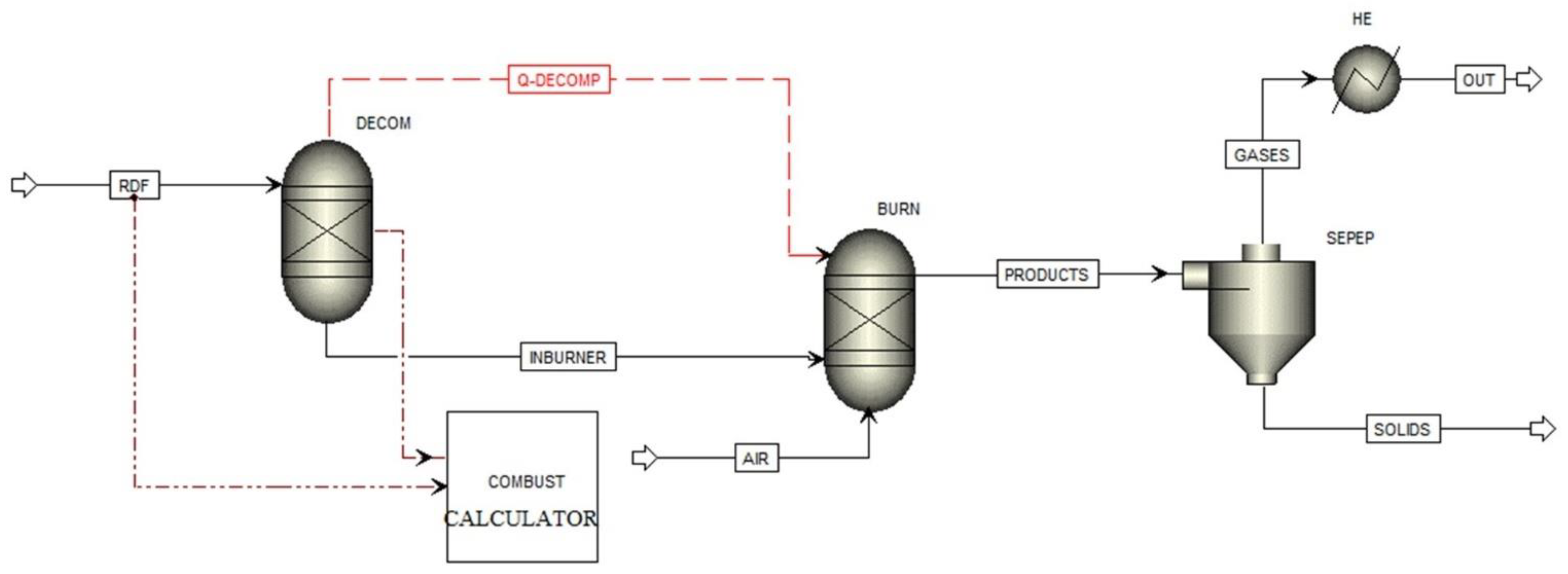
3.2. Simulation of the RDF Combustion Process

The simulations were made only for stream A, as it had a better quality than stream B (see statistical analysis above).

Table 13. Summary of obtained results.

Stream	Temperature t	Pressure p	Specific Enthalpy h	Density r	Mass Flow rate $\dot{\mathbf{m}}$
	(°C)	(bar)	(kJ/kg)	(kg/m3)	(kg/h)
RDF	21	1.01	−7510.80	1277.1200	1000.00
PRODUCTS	850	1.01	−430.43	0.3190	17606.00
AIR	21	1.01	−4.06	1.1900	16606.00
GASES	850	1.01	−441.22	0.3185	17575.90
OUT	150	1.01	−1222.16	0.8450	17575.90
SOLIDS	850	1.01	29.67	3486.8800	30.12

summarizes the parameters of individual streams at the characteristic points of the analyzed process.

The simulation shows that for the assumed conditions, about 3.85 kWh of heat can theoretically be obtained from each kilogram of RDF. It was calculated that for the examined waste stream A, each burnt kilogram of RDF will produce: NO_x = 12.95 mmol_NOx/g_RDF, SO_X = 0.0328 mmol_SOx/g_RDF, for CO₂ = 49.31 mmol_CO2/g_RDF.

These values are hypothetical specific emissions of a given gas per 1 kg of RDF burnt. This makes it possible to compare the specific emissions of different fuels. In reality, the heat output that can be recovered is likely to be less than simulated, compared to the assumption that about 3.85 kWh (13.860 MJ/kg) of heat can be obtained. An LHV of more than 11 MJ/kg generally ensures the energy efficiency of combustion, allowing the process to qualify for energy recovery [35]. The literature review shows that this value ranges from 2.5 to 4.3 kWh for each kg of RDF burnt. This is due to the fact that a higher proportion of ash was obtained when the samples were tested.

4. Summary

Undoubtedly, one advantage of RDF is its wide availability and the fact that its utilization is necessary for environmental reasons. Therefore, the quality of RDF composition and energy efficiency of this fuel needs to be assessed, which has been performed in this study. It was found that using statistical analysis and energy assessment by estimating the HHV, it is possible to determine the quality of waste (by comparing two waste streams) and usability as fuel: a heat yield of 13.860 MJ/kg is comparable to the combustion heat from average quality wood (Table 1).

Based on observations, simulations and analysis of statistical data, it can be concluded that:

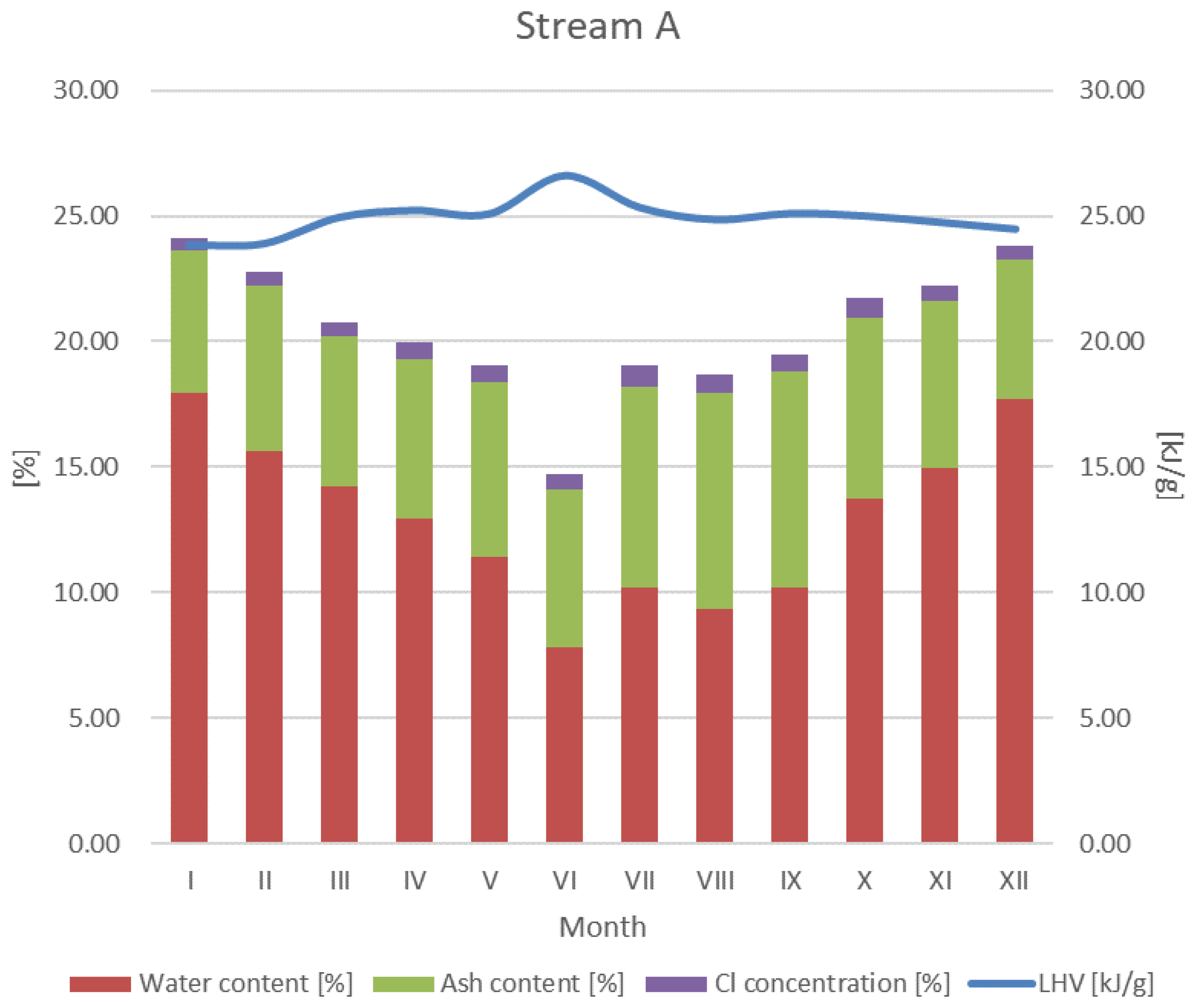
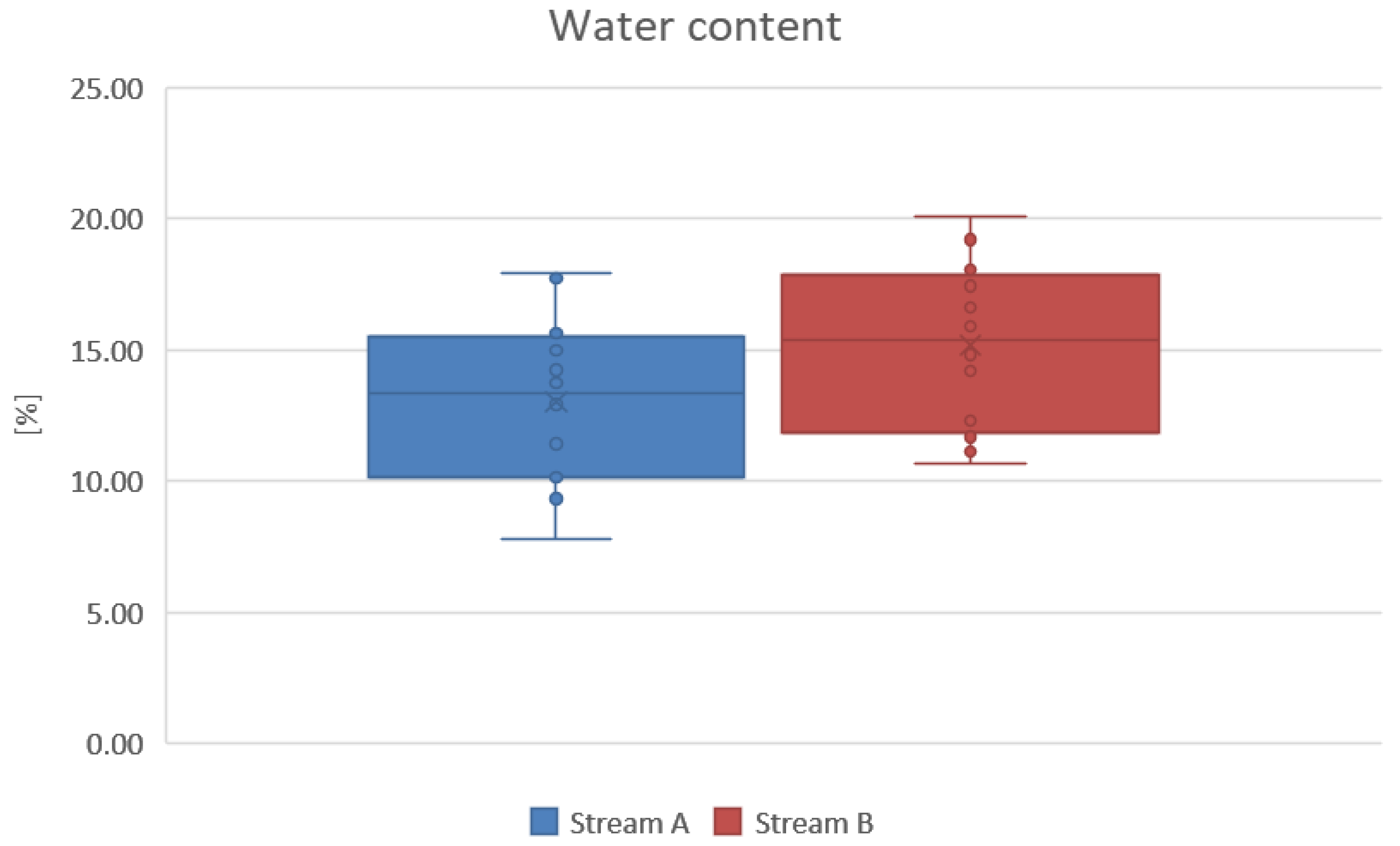
• the water content of the waste stream significantly affects its LHV and is dependent on the month of the year in which the samples were taken, behaving similarly in both streams. In the summer months (Table 6 and Table 7—June, July and August), the water content was, on average, about 50% lower (about 56% in stream A and about 47% in stream B) than in the autumn and winter months;
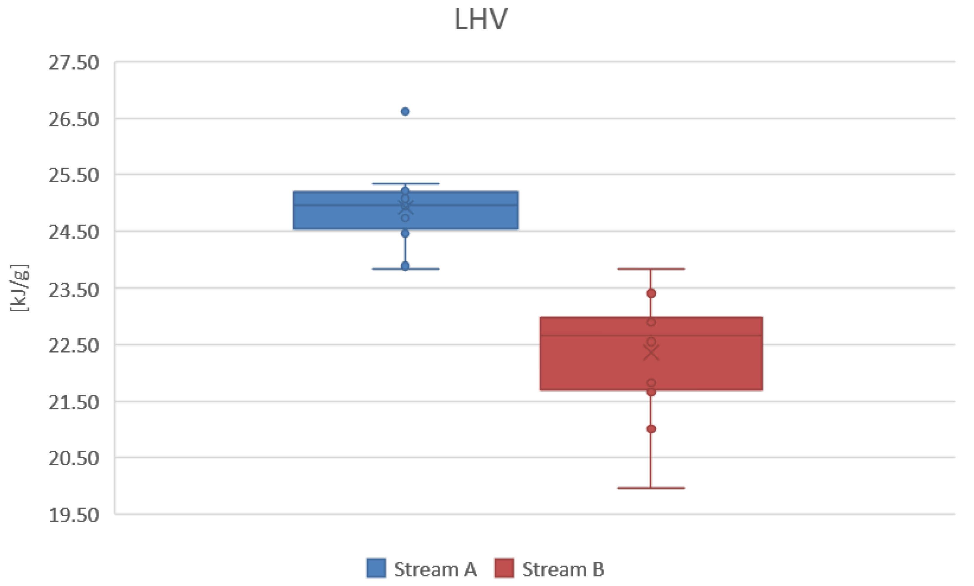
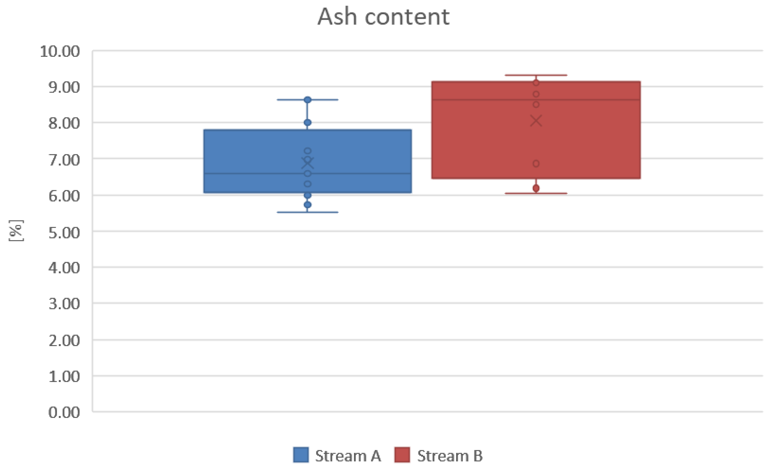
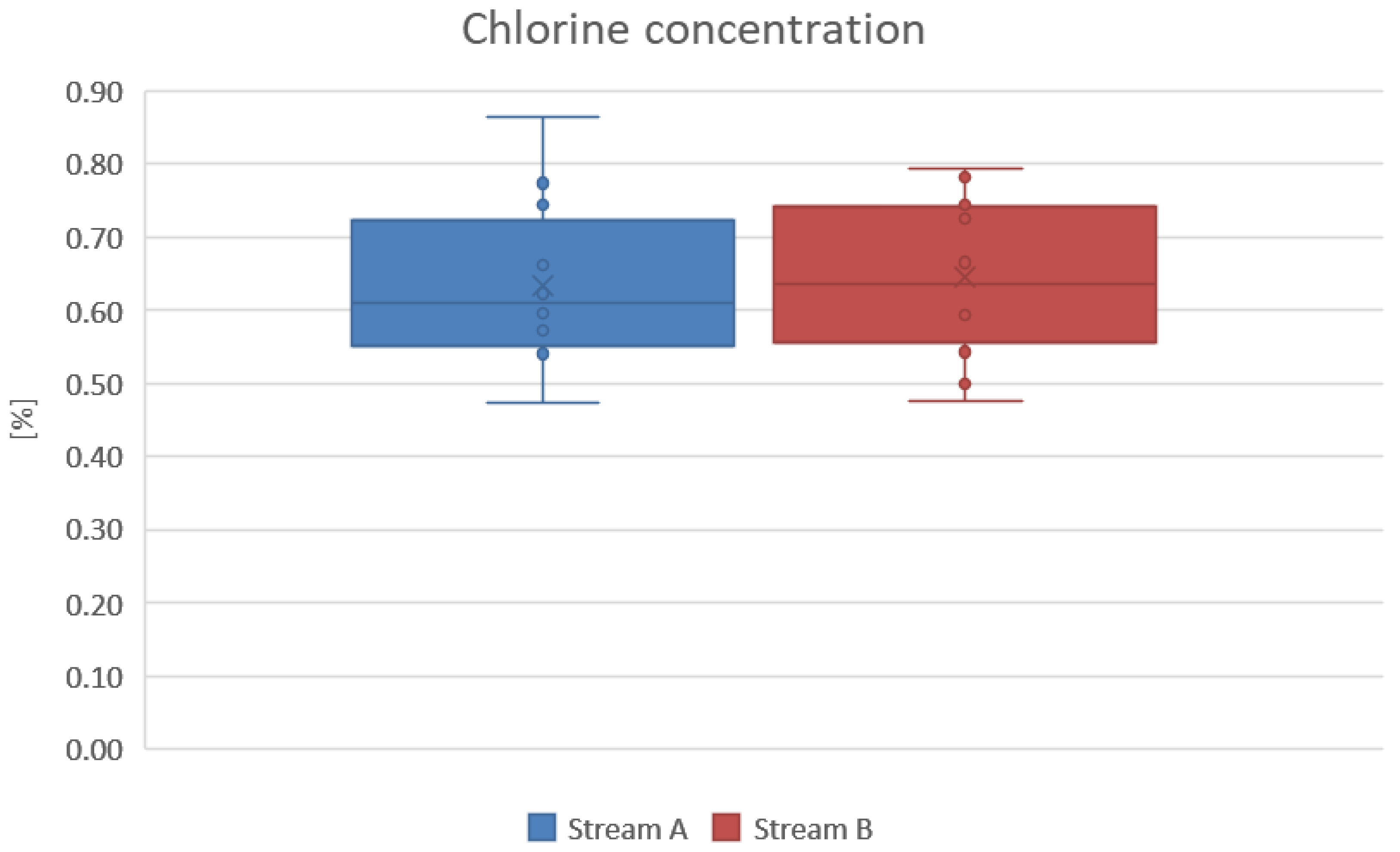
• analysis of the box plots of the parameters (Figure 4, Figure 5, Figure 6 and Figure 7) confirms that stream A has significantly better parameters than stream B. Stream A has a higher average LHV and lower average water content; its ash content is predictable as it follows a normal distribution. Furthermore, it can be concluded that the chlorine concentration is independent of the stream;
• the lack of significant correlation between the LHV of the streams confirms the earlier conclusion that stream A is significantly better than stream B in terms of performance for the RDF combustion process. This is probably related to the origin of the streams. Stream B consisted of industrial packaging waste, automotive waste, bulky items and mixed municipal waste, while stream A consisted of pre-sorted waste, where packaging waste from the food industry, post-production polymer waste and municipal waste were separated;
• simulations show that the heat yield (under the assumed conditions) for the combustion of RDF waste in stream A is approximately 3.85 kWh (13.860 MJ) for each kg of combusted fuel;
• for waste stream A under consideration, each kilogram of incinerated RDF will generate: NO_x = 12.95 mmol_NOx/g_RDF, SO_x = 0.0328 mmol_SOx/g_RDF and CO₂ compounds = 49.31 mmol_CO2/g_RDF.

This significantly pollutes the atmosphere and requires the application of specialized treatment systems.

The authors intend to further investigate the problem of emitting undesirable compounds, quantify them and describe the pyrolysis of RDF waste.

References

1. Monthly Bulletin of Statistics Online. Available online: https://unstats.un.org/unsd/mbs/app/DataSearchTable.aspx (accessed on 8 April 2022).
2. Magrini, C.; D’Addato, F.; Bonoli, A. Municipal Solid Waste Prevention: A Review of Market-Based Instruments in Six European Union Countries. Waste Manag. Res. 2020, 38, 3–22. [Google Scholar] [CrossRef] [PubMed]
3. Czarnecka-Komorowska, D.; Grześkowiak, K.; Popielarski, P.; Barczewski, M.; Gawdzińska, K.; Popławski, M. Polyethylene Wax Modified by Organoclay Bentonite Used in the Lost-Wax Casting Process: Processing−Structure−Property Relationships. Materials 2020, 13, 2255. [Google Scholar] [CrossRef] [PubMed]
4. Piesowicz, E.; Irska, I.; Bryll, K.; Gawdzinska, K.; Bratychak, M. Poly(Butylene Terephthalate/Carbon Nanotubes Nanocomposites. Part II. Structure and Properties. Polimery 2016, 61, 24–30. [Google Scholar] [CrossRef]
5. European Plastics Converters 2014/2015. Available online: https://plasticseurope.org/de/wp-content/uploads/sites/3/2021/11/2014-Plastics-the-facts.pdf (accessed on 29 March 2022).
6. Czarnecka-Komorowska, D.; Nowak-Grzebyta, J.; Gawdzińska, K.; Mysiukiewicz, O.; Tomasik, M. Polyethylene/Polyamide Blends Made of Waste with Compatibilizer: Processing, Morphology, Rheological and Thermo-Mechanical Behavior. Polymers 2021, 13, 2385. [Google Scholar] [CrossRef]
7. Jaglarz, G.; Generowicz, A. Energy Characteristics of Municipal Waste after Processes Recovery and Recycling. Econ. Environ. 2015, 2, 154–165. (In Polish) [Google Scholar]
8. Czarnecka-Komorowska, D.; Tomasik, M.; Thakur, V.K.; Kostecka, E.; Rydzkowski, T.; Jursa-Kulesza, J.; Bryll, K.; Mysłowski, J.; Gawdzińska, K. Biocomposite Composting Based on the Sugar-Protein Condensation Theory. Ind. Crop. Prod. 2022, 183, 114974. [Google Scholar] [CrossRef]
9. Czarnecka-Komorowska, D.; Kanciak, W.; Barczewski, M.; Barczewski, R.; Regulski, R.; Sędziak, D.; Jędryczka, C. Recycling of Plastics from Cable Waste from Automotive Industry in Poland as an Approach to the Circular Economy. Polymers 2021, 13, 3845. [Google Scholar] [CrossRef]
10. Wróblewska-Krepsztul, J.; Rydzkowski, T.; Borowski, G.; Szczypiński, M.; Klepka, T.; Thakur, V.K. Recent Progress in Biodegradable Polymers and Nanocomposite-Based Packaging Materials for Sustainable Environment. Int. J. Polym. Anal. Charact. 2018, 23, 383–395. [Google Scholar] [CrossRef]
11. What Waste to Recycle? Available online: https://naszesmieci.mos.gov.pl/materialy/artykuly/144-jakie-odpady-do-recyklingu (accessed on 27 March 2022). (In Polish)
12. Rana, A.K.; Thakur, M.K.; Saini, A.K.; Mokhta, S.K.; Moradi, O.; Rydzkowski, T.; Alsanie, W.F.; Wang, Q.; Grammatikos, S.; Thakur, V.K. Recent Developments in Microbial Degradation of Polypropylene: Integrated Approaches towards a Sustainable Environment. Sci. Total Environ. 2022, 826, 154056. [Google Scholar] [CrossRef]
13. Paszkowski, J.; Domański, M.; Caban, J.; Zarajczyk, J.; Pristavka, M.; Findura, P. The Use of Refuse Derived Fuel (RDF) in the Power Industry. Agric. Eng. 2020, 24, 83–90. [Google Scholar] [CrossRef]
14. Zamorowska, K. RDF Is Waiting for Its Chance and Companies Are Waiting for RDF. Available online: https://www.teraz-srodowisko.pl/aktualnosci/RDF-czeka-na-swoja-szanse-a-przedsiebiorstwa-czekaja-na-RDF-6142.html (accessed on 29 March 2022). (In Polish).
15. Fuels. Available online: http://zss.lublin.eu/wp-content/uploads/2016/11/20.-Paliwa-silnikowe.pdf (accessed on 25 April 2022). (In Polish).
16. Practical Table of Calorific Value of Various Fuels with an Overview. Available online: https://kb.pl/porady/praktyczna-tabela-wartosci-opalowej-roznych-paliw-z-omowieniem/?fbclid=IwAR3xE0ubI_5anQKjABbRIwuDSRbBbo9VTysEJolce-PkIRrYuRTeFpk03BY (accessed on 25 April 2022). (In Polish).
17. Mróz, J. Recycling and Utilization of Waste Materials in Metallurgical Units; Częstochowa University of Technology Publishing House: Częstochowa, Poland, 2006. (In Polish) [Google Scholar]
18. Janowska, G.; Przygocki, W.; Włochowicz, A. Flammability of Polymers and Polymeric Materials; WNT: Warsaw, Poland, 2007. (In Polish) [Google Scholar]
19. Burzynski, M.; Paszkiewicz, S.; Piesowicz, E.; Irska, I.; Dydek, K.; Boczkowska, A.; Wysocki, S.; Sieminski, J. Comparison Study of the Influence of Carbon and Halloysite Nanotubes on the Preparation and Rheological Behavior of Linear Low Density Polyethylene. Polimery 2020, 65, 95–98. [Google Scholar] [CrossRef]
20. Davy, J., VI. On a Gaseous Compound of Carbonic Oxide and Chlorine. Philos. Trans. R. Soc. Lond. 1812, 102, 144–151. [Google Scholar] [CrossRef] [Green Version]
21. Olszowiec, P. Waste Incineration Plants Are Becoming Safer. PCV: To Burn or... Not to Burn? Energ. Gigawat 2014, 1–2. (In Polish) [Google Scholar]
22. Rajca, P.; Zajemska, M. Assessment of the Possibility of Using Rdf Fuel for Energy Purposes. Rynek Energii 2018, 4, 29–37. (In Polish) [Google Scholar]
23. Lombardi, L.; Carnevale, E.; Corti, A. A Review of Technologies and Performances of Thermal Treatment Systems for Energy Recovery from Waste. Waste Manag. 2015, 37, 26–44. [Google Scholar] [CrossRef]
24. Zychlinski, W.; Fischmann, J. Vinylchloride from 1,2-Dichloroethane—Annotations to the Present State of Knowledge. Chemishe Tech. 1990, 42, 321–324. [Google Scholar]
25. Paszkiewicz, S.; Irska, I.; Taraghi, I.; Piesowicz, E.; Sieminski, J.; Zawisza, K.; Pypeć, K.; Dobrzynska, R.; Terelak-Tymczyna, A.; Stateczny, K.; et al. Halloysite Nanotubes and Silane-Treated Alumina Trihydrate Hybrid Flame Retardant System for High-Performance Cable Insulation. Polymers 2021, 13, 2134. [Google Scholar] [CrossRef] [PubMed]
26. Lachowicz, M.; Gacki, M.; Moskwik, K. Fuels and Engines of Economic Growth. The Impact of Raw Material Prices and Energy Production on Poland; Instytut Jagielloński: Warsaw, Poland, 2020. (In Polish) [Google Scholar]
27. RDF—A Rescue (Not Only) for the Polish Energy Sector? Available online: https://www.fortum.pl/media/2020/10/rdf-ratunek-nie-tylko-dla-polskiej-energetyki (accessed on 26 May 2022). (In Polish).
28. Adamczuk-Poskart, M. Possibilities of Using Computer Simulation Methods for Modelling Combustion Processes. Metallurgist 2010, 12, 736–739. (In Polish) [Google Scholar]
29. Pilar González-Vázquez, M.; Rubiera, F.; Pevida, C.; Pio, D.T.; Tarelho, L.A.C. Thermodynamic Analysis of Biomass Gasification Using Aspen Plus: Comparison of Stoichiometric and Non-Stoichiometric Models. Energies 2021, 14, 189. [Google Scholar] [CrossRef]
30. Chen, C.; Mao, J.; Liu, X.; Tian, S.; Song, L. Modelling and Combustion Optimization of Coal-Fired Heating Boiler Based on Thermal Network. Therm. Sci. 2021, 25, 3133–3140. [Google Scholar] [CrossRef]
31. Zhang, Y. Trace Elements Characteristics of Ultra-Low Emission Coal-Fired Power Plants. In Advances in Ultra-Low Emission Control Technologies for Coal-Fired Power Plants; Elsevier: Amsterdam, The Netherlands, 2019; pp. 199–239. [Google Scholar]
32. Suárez-Ruiz, I.; Ward, C.R. Basic Factors Controlling Coal Quality and Technological Behavior of Coal. In Applied Coal Petrology; Elsevier: Amsterdam, The Netherlands, 2008; pp. 19–59. [Google Scholar]
33. Ronsse, F.; Nachenius, R.W.; Prins, W. Carbonization of Biomass. In Recent Advances in Thermo-Chemical Conversion of Biomass; Elsevier: Amsterdam, The Netherlands, 2015; pp. 293–324. [Google Scholar]
34. Li, H.; Tang, K. A Comprehensive Study of Drop-in Alternative Mixtures for R134a in a Mobile Air-Conditioning System. Appl. Therm. Eng. 2022, 203, 117914. [Google Scholar] [CrossRef]
35. Sidełko, R. Application of Technological Processes to Create a Unitary Model for Energy Recovery from Municipal Waste. Energies 2021, 14, 3118. [Google Scholar] [CrossRef]
36. Azam, M.; Jahromy, S.S.; Raza, W.; Raza, N.; Lee, S.S.; Kim, K.-H.; Winter, F. Status, Characterization, and Potential Utilization of Municipal Solid Waste as Renewable Energy Source: Lahore Case Study in Pakistan. Environ. Int. 2020, 134, 105291. [Google Scholar] [CrossRef] [PubMed]
37. Kotulski, Z.; Szczepiński, W. Error Calculus for Engineers; WNT: Warsaw, Poland, 2004. (In Polish) [Google Scholar]
38. Bobrowski, D.; Maćkowiak-Łybacka, K. Selected Methods of Statistical Inference; Publishing House of the Poznań University of Technology: Poznań, Poland, 2006. (In Polish) [Google Scholar]
39. Boryczko, A. Fundamentals of Measurements of Mechanical Quantities; Wydawnictwo Politechniki Gdańskiej: Gdańsk, Poland, 2010. (In Polish) [Google Scholar]
Figure 1. Simulation diagram based on Aspen Plus software.
Energies 15 09560 g001
Figure 2. Summary of stream A parameters.
Energies 15 09560 g002
Figure 3. Summary of stream B parameters.
Energies 15 09560 g003
Figure 4. Comparison of box plots of the LHV for streams A and B.
Energies 15 09560 g004
Figure 5. Comparison of water content box plots for streams A and B.
Energies 15 09560 g005
Figure 6. Comparison of box plots of ash content for streams A and B.
Energies 15 09560 g006
Figure 7. Comparison of box plots of chlorine concentration for streams A and B.
Energies 15 09560 g007