Article

Levelling the Photovoltaic Power Profile with the Integrated Energy Storage System

by
Alberto Benato
,
Francesco De Vanna
*,† and
Anna Stoppato
Department of Industrial Engineering, University of Padova, 35122 Padova, Italy
*
Author to whom correspondence should be addressed.
These authors contributed equally to this work.
Energies 2022, 15(24), 9521; https://doi.org/10.3390/en15249521
Submission received: 25 September 2022 / Revised: 10 November 2022 / Accepted: 12 December 2022 / Published: 15 December 2022
(This article belongs to the Collection Renewable Energy and Energy Storage Systems)

Abstract

:
The extensive penetration in the energy mix of variable renewable energy sources, such as wind and solar, guarantees boosting of the transition toward a decarbonized and sustainable energy system as well as tackling of climate targets. However, the instability and unpredictability of such sources predominantly affect their plant production. Thus, utility-scale energy storage is required to aid in balancing supply and demand and, as a result, to prevent unbalances that might cause issues at different grid levels. In the present study, the authors’ patented energy storage technology, known as Integrated Energy Storage System (I-ESS), is combined with a 10 MWp solar plant. The PV plant and the I-ESS unit function as a Virtual Power Plant (VPP). The selected VPP management strategy attempts to optimize the daily hours during which the plant supplies steady power output. Numerical simulations show that the VPP plant can effectively smooth the PV peak and manage the power supply. In particular, by the definition of a novel metric expressing the ratio between regular hours of power provided to the grid plus the energy stored in the backup unit and the total number of hours in a year, the results show that the VPP regularity is relatively high in terms of PV output, ranging from a low of 50% in December to a high of 87% in August. Thus, the proposed VPP arrangement seems to be a promising technology for pushing toward the carbon-neutral transition.

1. Introduction

The socioeconomic growth of nations is inextricably tied to energy availability or, in other words, it is dependent on having access to a variety of energy sources at the lowest feasible cost. Currently, only fossil fuels such as coal, crude oil and natural gas can provide this requirement. However, population expansion is hastening energy consumption and increasing the demand for and use of fossil fuels. Nonetheless, such a tendency raises pollutant emissions and exacerbates global climate change. The worldwide increase in CO 2 and greenhouse gas emissions, as well as the repercussions of climate change, have compelled global society to respond by demanding tangible and practical steps capable of altering how energy is generated and natural resources are managed. To this end, two worldwide treaties were signed: the Kyoto Protocol [1] and the Paris Agreement [2]. Despite the world treaties, only the member state of the European Union (EU) agreed to set stringent and binding targets for the years 2020 [3], 2030 [4] and 2050 [5] to push the energy transition toward a renewable-based economy. Notwithstanding the achievement of the targets set for 2020 [3] and the strenuous efforts to build a sustainable and decarbonized power generation system, more than 77% of the EU’s greenhouse gas emissions still come from the production and use of energy [6]; a considerable share that can compromise the entire ambitious plan of becoming climate neutral by 2050. Therefore, to speed up the installations of renewable-based plants, cut CO 2 and greenhouse gas emissions and jump-start the economy after the devastating COVID-19 waves, the EU established the European Green Deal (EGD) [7]. The plan set ambitious greenhouse gas emission cuts. The Paris Agreement set a reduction in CO 2 of at least of 40% by 2030 compared to 1990 levels, while the EGD increased that target to at least 55%. Obviously, this is a big challenge for the EU but relies on fine achievements. One above all is the emissions reduction reached in 2020 compared to the target fixed for that year in 2008. The goal was a reduction of 20%, but, already in 2019, the registered reduction was equal to 24%. The percentage increased to 31% in 2020 (partially due to the COVID-19 pandemic). Thus, although achieving carbon neutrality in fewer than 30 years may be difficult, there will be many advantages. Instead of using fossil fuels, the power industry will rely on Renewable Energy Sources (RESs). Citizens may generate their own energy and the proportion of RESs in total energy consumption may be increased up to 32%. The supplies will be secured and guaranteed to be affordable. The energy market will be digitalized, integrated and networked. The notion of energy efficiency will expand and the energy performance of the building will be improved.
We have therefore understood that the EU’s objectives are far from simple, but we must now understand what it means for a member state to implement such maneuvers. Let us take Italy as an example. To fulfill the assigned goals, Italy has to add 10 GW of wind (of which 0.9 GW will be offshore) and 30 GWp of solar (of which 0.88 GWp will be concentrated solar power) by 2030 [8]. This means jumping from 10.90 GW of wind and 21.65 GWp of solar installed in 2020 to 23.23 GW and 52 GWp, respectively [9], a rise that could boost renewable electricity production from 41.7% up to 55%, with significant benefits in terms of greenhouse gas reduction and security in energy supplies. Such a transition is increasingly essential, especially after 24 February, 2022, when Russia started military aggression against Ukraine. From that date, the world’s energy and economic system equilibrium has been completely disrupted and EU authorities were pushed to amend sanctions on Russia in light of supporting Ukraine’s resistance. Such a set of political maneuvers provoked a cut in Russia’s natural gas export, forcing the European Commission to act to avoid an energy crisis [10] rapidly. The result is the REPower EU [11]: a plan to rapidly reduce dependence on Russian fossil fuels and fast forward the green transition. This plan intends to increase wind and solar installation, particularly in countries like Italy, where these resources are abundant and the dependence on Russian natural gas is considerable compared to other EU members. However, because of such sources’ changeable and unpredictable character, a synergy between power deployment and storage capacity installations is required. This is the only measure that can assist balance supply and demand without experiencing significant and unexpected power swings, which may cause management and control issues, device malfunctions and local to worldwide blackouts. As previously stated, if Italy is taken as an example, to allow a grid-safe operation after adding other 10 GW of wind and 30 GWp of solar, estimations indicate the need to add approximately 6 GW of centered storage and 4 GW of distributed storage [8], a requirement of new storage capacity that can not be covered only with pumped hydro and battery energy storage. Therefore, there is a demand for conceptualizing and designing alternative energy storage systems able to be installed near renewable plants and capable of storing large amounts of energy. Additionally, it can be beneficial that these new storage facilities exhibit a low or even null environmental impact and a capability to use the fossil-based power units’ sites, devices and infrastructures. The latter features can revamp conventional plants fed by fossil fuels in storage units, an action that prevents land and raw material consumption.
Baring in mind the requirements and the socio-economical constraints mentioned above, the authors have developed the so-called Integrated Energy Storage System (I-ESS): a storage unit embeddable into in-decommissioning fossil thermal power plants and in the location of wind or solar facilities [12,13]. The plant stores electricity as sensible heat in a high-temperature artificial tank consisting of a solid packed bed that acts as a Thermal Energy Storage (TES). The I-ESS plant is an open-cycle adopting air as a working fluid in both storing and regenerating mode. The storing scheme comprises a high-temperature tank, a fan, an electric heater, an electric motor and a heat exchanger. On the other hand, the re-generation unit consists of a gas turbine in which the high-temperature tank replaces the combustion chamber. Unlike other energy storage technologies such as pumped hydro and compressed air energy storage, the I-ESS plant has no geographical constraints and does not need a steady water flow like pumped hydro or a natural gas stream like compressed air energy storage. The I-ESS unit has a longer cycle life than storage batteries and its design has a lower scheme complexity than Pumped Thermal Energy Storage (PTES). Despite past tests proving the I-ESS plant’s practicality, more research into the plant’s ability to function in conjunction with a variable renewable-based facility is required. To this end, the authors selected to couple the I-ESS unit with a PhotoVoltaic (PV) facility characterized by a peak power of 10 MW. The I-ESS storage unit and the PV facility act as a Virtual Power Plant (VPP), being perceived by the electric grid as a unique generation unit. In this study, the VPP is managed so that it provides constant power to the grid for the maximum number of hours possible throughout the year. Such a management strategy avoids the typical daily power fluctuations of solar energy. To the best of the authors’ knowledge, there is no equivalent research in the literature in terms of both plant layout and management approach, making this study a genuine pioneering contribution in the field.
The vast majority of the investigations available in the literature, in fact, focused on developing new TES-based plant arrangements and evaluating their energy performance. The first investigation dated back to 2010 and was performed by Desrues et al. [14]. The study described a PTES system for large-scale electricity storage. During the charge, the unit acts as a high-temperature heat pump cycle, while it works as a thermal engine during the delivery phase. The electricity is converted into heat through a compressor and stored in cold and hot tanks. The simulations demonstrated the plant’s capability of storing 602.6 MWh. The charge and discharge times were 6 h 3 min and 5 h 52 min, respectively, while the storage efficiency reached 66.7%. A year later, Howes [15] presented a similar configuration, but, in his conceptualization, the PTES unit could generate 2 MW and store 16 MWh. Based on this study, the author claimed that PTES has vast potential due to its high efficiency and low costs. Simultaneously to Howes [15], White [16] conducted an investigation on PTES to estimate the thermal reservoirs’ thermodynamic losses. He concluded that two sources of losses could be defined: thermal losses and pressure losses. The former are associated with thermodynamics irreversibility, while frictional mechanical effects cause the latter. Both of them cannot be neglected and a set of correlations was proposed for their estimations. Considering the promising findings, in the period 2013–2018, White and his research team performed a set of investigations on PTES devoted to analyzing (i) the entire cycle performance [17], (ii) the wave propagation and the losses in packed bed [18], (iii) the design of the plant [19], of the reservoirs [20] and the backed bed flow path [21]. In the same time frame, Thess [22], Ni and Caram [23], Guo et al. [24], Abarr et al. [25,26] and Benato [27] also analyzed the PTES configuration with the aim of assessing the PTES energy performance and find the best working fluid and thermodynamic conditions.
Contrary to the previous studies, Benato and Stoppato [28] studied the influence on the PTES energy and economic performance of the storage material type and the maximum cycle temperature while Wang et al. [29] analyzed, in an initial study, the influence of the mass flow rate unbalances in the packed bed and, then, they proposed an innovative management strategy for the Brayton-cycle-based pumped heat electricity storage able to reduce by 1.8 the storage size [30].
More recently, Zhao et al. [31] conducted a parametric design optimization to find the best PTES configuration working fluids and storage media from a thermodynamic perspective, while Albert et al. [32] evaluated the operation and the performance of a Brayton PTES with additional latent storage. Bahzad et al. [33] proposed two novel energy storage systems intending to reduce the cost per unit of energy stored. The first integrates the PTES with the chemical looping technologies, while the second merges the first system with an open-cycle gas turbine. The performed techno-economic assessment shows that both systems’ round-trip efficiency reaches 77%, but the daily profit of the second integrated plant is between 4.9% and 72.9% higher than the system coupling the PTES with the chemical looping technologies. Zhang et al. [34] compared a PTES system with indirect thermal energy storage and a direct one. The results show that, despite a lower round-trip efficiency, the Indirect PTES is advantageous owing to its low installation cost when its electricity storage duration exceeds 6 h. In terms of capital cost, the latter configuration guarantees a 40% reduction compared to Direct PTES. After this preliminary investigation, Zhang et al. [34] designed a 10 MW Indirect PTES system and found that the optimum round-trip efficiency and energy density are approximately 65% and 26 kWh m−3, respectively. They also noted that the research provides a theoretical basis for designing and optimizing high-efficiency and low-capital-cost PTES systems. On the other hand, Wang et al. [35] developed an optimizer based on the exergy method for a Joule–Brayton cycle-based PTES system. The study demonstrated that the maximum working temperature and the efficiency of the turbomachines are positively correlated to the round-trip efficiency and the energy storage density. Moreover, the optimal pressure ratio must be determined to balance efficiency and energy storage density. The above-mentioned analyses and the optimization provide a theoretical approach for the future design of such systems.
In the literature, several reviews are also available. For example, Benato et al. [36] presented the state-of-the-art and the future development of the sensible heat thermal electricity storage systems while, in a later study, they analyzed and compared the pumped thermal electricity storage with other large-scale storage technology underlying both the characteristics and the barriers that can limit the spread of this technology [37]. Moreover, Smallbone et al. [38] compared PTES with other storage technologies, but the yardstick is the levelized cost of storage. In 2020, Dumont et al. [39] presented a state-of-the-art review of the Carnot Battery technology while, in 2022, Novotny et al. [40] focused their review on the commercial development of the Carnot Battery technology. Contrary to others, Liang et al. [41] performed a technical review of the key components for the Carnot Battery, focusing on technical barriers and the selection criteria.
Based on the performed literature survey, to the authors’ best knowledge, only Petrollese et al. [42] conducted an investigation involving a storage unit adopting a TES-based tank and a renewable-based plant combined in a VPP. Conversely, such literature has a more corroborated tradition in other fields, such as wind and pumped-hydro [43,44,45] or, more recently, wind and electric vehicle fleet [46,47]. In particular, Petrollese et al. [42] aimed to thermally integrate a PTES system with a Concentrating Solar Power (CSP) plant. The two sections operate with the same working fluid, share several components and can operate simultaneously or independently of each other. A TES system composed of three thermocline packed-bed tanks is included. Specific mathematical models were developed to simulate the performance of the integrated PTES-CSP plant under design conditions and to evaluate the thermal profiles of the TES tanks. As a case study, an integrated PTES-CSP system characterized by a nameplate power of 5 MW with a design storage capacity of four equivalent hours was considered. The influence of the main design parameters, namely the pressure ratio and the operating temperatures of the TES system, on the leading performance indices was discussed. As is evident, the investigation is profoundly different from the study proposed in the present study since, in this investigation, the focus is not on the I-ESS performance but the VPP one. In addition, the renewable facility, in this case, is a PV and the storage unit is the I-ESS instead of a conventional PTES unit. The I-ESS is an authors’ patented configuration [48].
The rest of the work is organized as follows. Section 2 describes the power plant in terms of the I-ESS characteristics, numerical modeling and VPP arrangements. Results are presented in Section 3, while concluding remarks are given in Section 4.

2. The Power Plant Description

2.1. The Integrated Energy Storage System

The key element of the present VPP proposal is the I-ESS unit. This is a patented configuration established by the authors based on the PTES idea but with the key benefits and shortcomings of that technology in mind. The authors also wanted to suggest a low-complexity storage unit that uses a freely accessible, non-toxic and non-flammable fluid, as well as a storage facility that can be installed near renewable facilities or embedded in underutilized/decommissioned fossil-based units. Furthermore, during the I-ESS conception, the authors contemplated using largely market-available energy-sector components (such as compressors, turbines, fans, tanks and so on) to make their storage system readily buildable. In the past, the authors first analyzed the complete storage plant [12,13] to assess the proposal’s performance and technical and economic feasibility. They then shifted their focus to the TES tank [49]. Both branches of the same study subject revealed the need for thorough mathematical models, particularly in putting the suggested technology to work for a variable renewable plant to smooth its production curve and minimize grid instabilities.
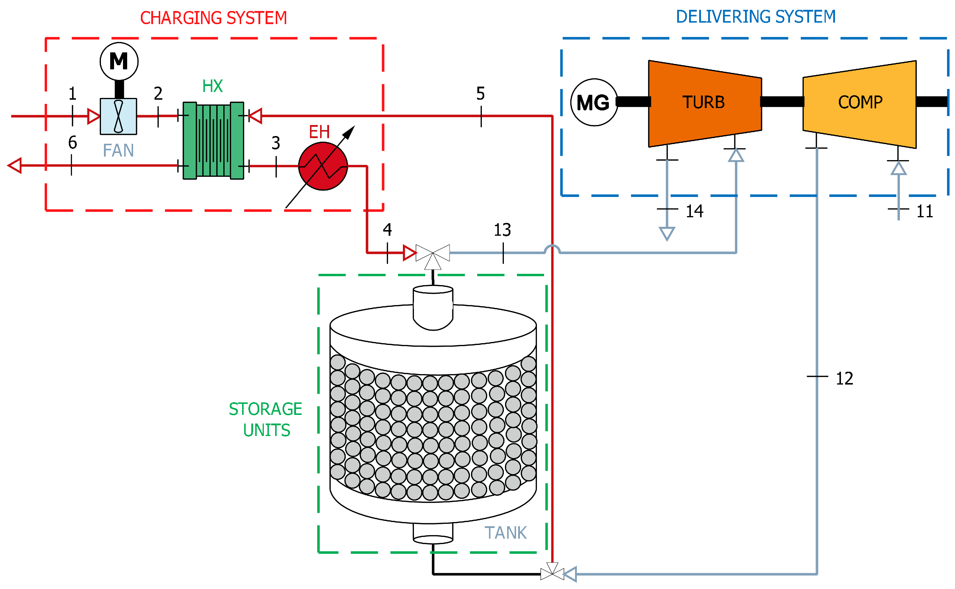
Figure 1 displays the I-ESS scheme. The design incorporates the components necessary to store electricity in the form of sensible heat as well as those that enable the thermal energy stored in the tank to be converted back into electricity. To store the power in the form of sensible heat, the system needs a fan (FAN), a heat exchanger (HX), an electric heater (EH) and a high-temperature storage tank (TANK). The plant is an open cycle, with air serving as the heat transfer fluid. The fan draws air from the surrounding environment (point 1) and pushes it to follow the path indicated by points 2 to 6. The operational fluid exiting the fan passes via the heat exchanger (way 2–3) and the electric heater (route 3–4). The electric heater is the heart of the storage unit because it turns excess power, such as that produced by solar or wind energy, into heat. In actuality, the device employs electrical energy to raise the air temperature from the state reached in point 3 to the highest possible value in the cycle (point 4). T4 corresponds to Tmax, the maximum cycle temperature.
This is an I-ESS plant design parameter that is chosen during the engineering phase based on the physical properties of the TES-packed bed storage material and the electric heater manufacturing technology. The latter is crucial since market-available electric heaters cannot attain temperatures greater than 1200 °C owing to a shortage of high-performance materials, limiting I-ESS performance. In contrast to PTES systems where the compressor turns power into heat, the electric heater enables T4 to remain constant and equal to Tmax regardless of the value assumed by the temperature in point 3. This distinguishing feature of the I-ESS unit ensures that the fluid is heated directly with electricity rather than employing the compression process irreversibly. A high-pressure ratio is obviously required to obtain a high temperature in PTES, which means high purchase costs for both the compressor and the storage tank. In the I-ESS plant, on the other hand, the design pressure established during the charge is equivalent to one that ensures airflow through the components while accounting for pressure losses. In a word, the electric heater insertion enables you to choose a low-pressure setting while retaining a high maximum cycle temperature.
The heated air that exits the electric heater in condition 4 enters the tank, which serves as the thermal energy storage unit. The tank is vertically structured to minimize buoyancy-driven thermal front instabilities and is composed of three elements: (i) The upper plenum. A crucial component for balancing the airflow and lowering its velocity. (ii) The packed bed, i.e., the TES device’s core. The packed bed stores electricity in the form of sensible heat and is composed of randomly packed spheres or a solid matrix with airflow channels. Aluminum oxide, titanium oxide, limestone, concrete, sand, masonry material and silica may all be used to make the solid matrix or the spheres. Depending on the specific heat and density of the material, the TES may be used to store heat at high or low temperatures and for a long or short period of time [50]. As a result, choosing the packed bed material and shape is critical for properly designing the TES and optimizing the I-ESS plant’s performance depending on the function needed by the grid. (iii) The plenum at the bottom. This tank section catches air and then delivers it through the pipe.
As said, the air enters the tank at condition 4 and flows through the packed bed. At the begging of the charging process, the packed bed material is at ambient temperature. Therefore, during its flow, the hot air heats the packed bed and, when it leaves the tank, its temperature (T5) and pressure (p5) are both lower than those reached in point 4. It is also worth noting that, in comparison to the PTES, the I-ESS plant has a single tank (the hot one), while the PTES has both cold and hot storage. Before being discharged into the environment, the air is driven via a heat exchanger to enable pre-heating of the air entering the electric heater and further cooling the air exiting the I-ESS unit. In contrast to PTES, as previously stated, the I-ESS is an open cycle utilizing air rather than a closed loop using argon.
When the grid needs electricity, the I-ESS plant operates in discharging mode. The re-generation unit consists of a gas turbine with thermal storage in place of a combustion chamber. The compressor draws air from the surroundings at ambient conditions (point 11). The compressed air is then transported to the TES tank to be heated by the heat stored in the packed bed material (point 12). The air leaving the storage at condition 13 is expanded by the air turbine. After the expansion, the air is released into the environment. As for the charge layout, the delivery arrangement is also an open loop with unique storage. So, compared to PTES, the number of components is reduced, the working fluid is air and the plant management is less complex, with the gas turbine power unit being without the combustion chamber. There are also benefits in terms of costs compared to PTES and plant availability.

2.2. The Virtual Power Plant

A VPP is an aggregator that connects generators, loads and storage systems as a single entity to the grid. The VPP concept is vast since it may combine numerous types of distributed energy sources and can serve a variety of direct and indirect goals depending on the players involved and the marketplaces in which it works. The VPP in this study combines a variable renewable solar PV plant with the I-ESS unit specified in 
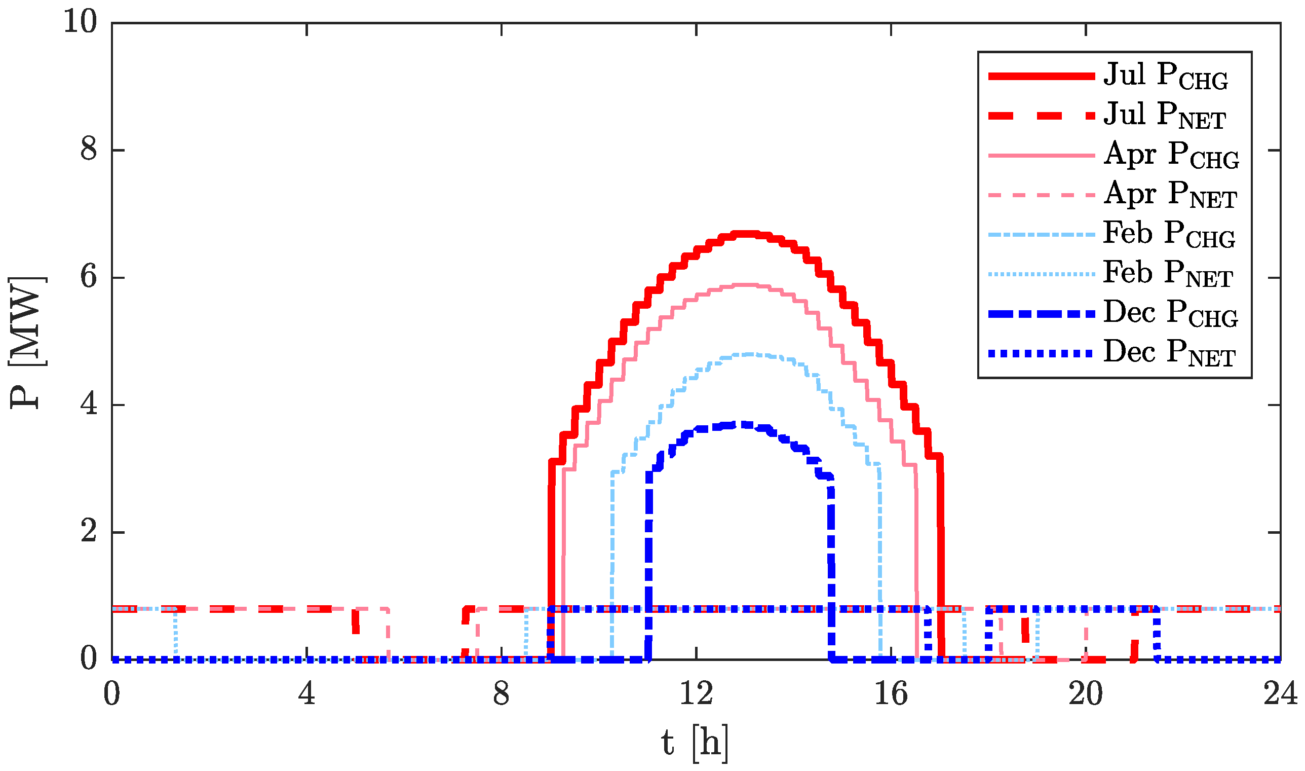
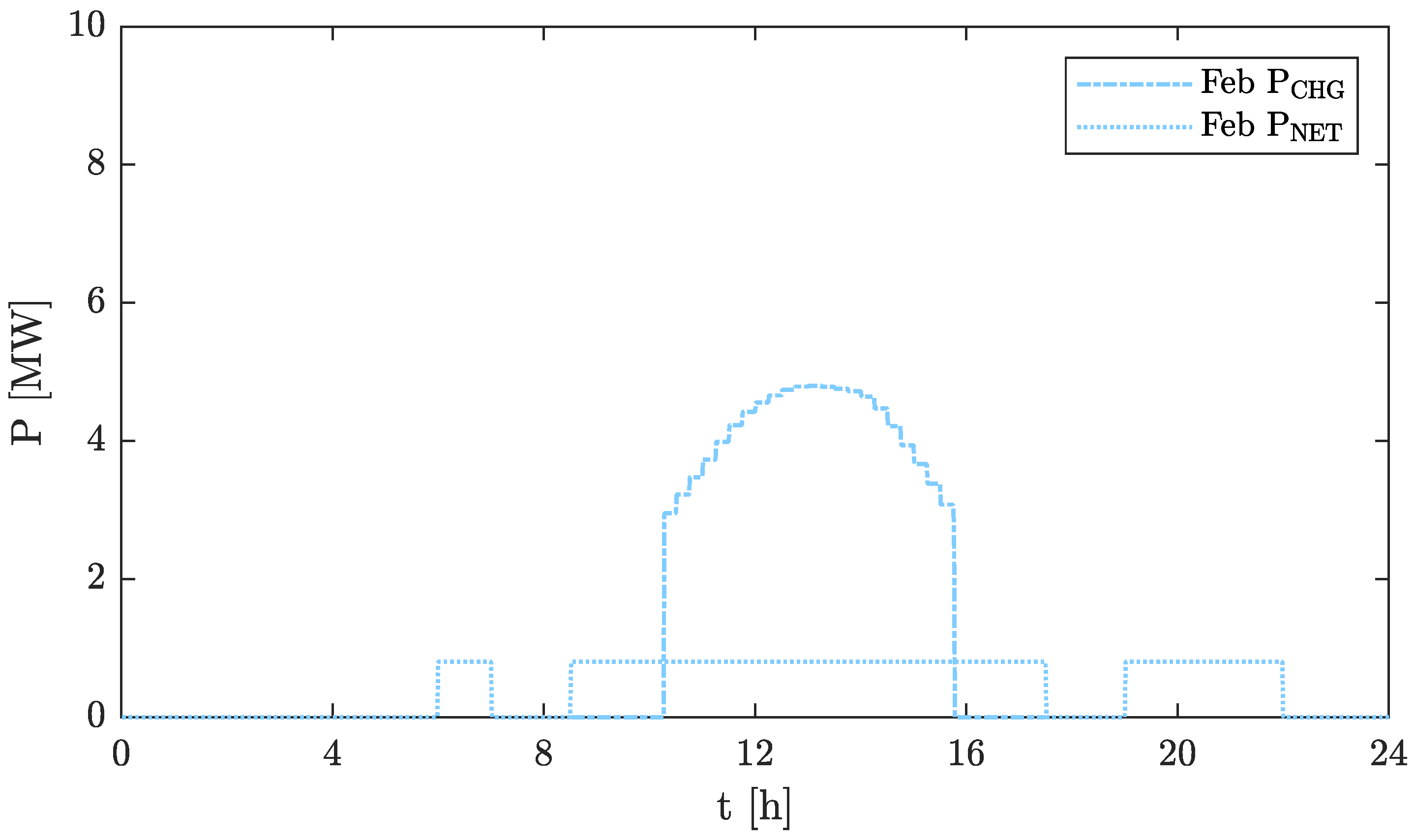
Section 2.1. The VPP’s goal is to prevent the traditional peak power during intense solar radiation times and the nighttime hours of null output. System operators, in fact, dislike situations that might cause instabilities in the electric grid. Thus, to achieve this purpose, a portion of the energy generated by the PV plant during peak output hours is immediately transferred to the electric grid, while the remainder is utilized to charge the I-ESS system’s storage tank when circumstances permit. During non-productive PV hours, the energy stored in the I-ESS tank as sensible heat is converted to electricity and provided to the grid at a steady power output. As a consequence of the PV aggregation with the I-ESS storage, the grid’s power profile becomes mostly constant. In the case under consideration, a management strategy is developed that allows the VPP to be viewed as a plant that provides programmable and constant power to the grid for the maximum number of hours per day, even though the generation comes from a variable renewable energy source. This is a network-related problem, as will be explained later. 
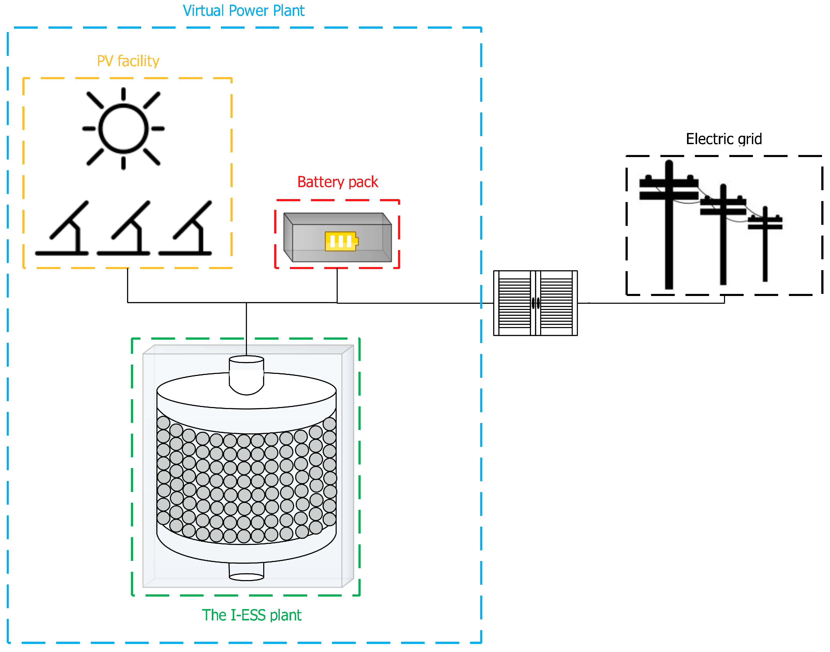
Figure 2 reports a sketch of the VPP.
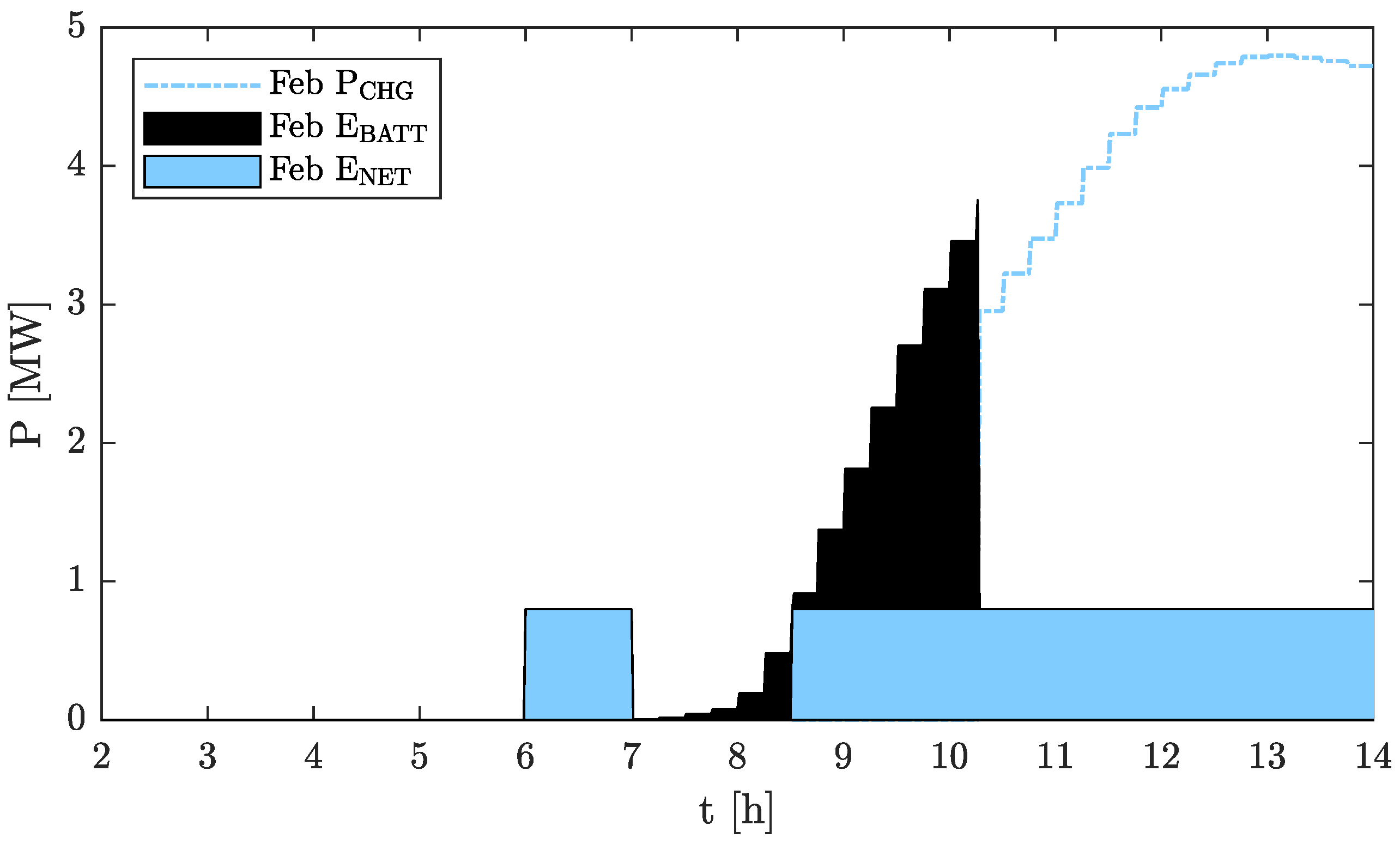
As can be seen, the plant also includes a battery pack. Such a device is required to store energy when the power provided by the PV is less than a predefined power and is also insufficient to charge the TES tank. Thus, the energy stored in batteries is utilized to start the I-ESS power train when the re-conversion phase begins. Considering the PV and I-ESS design characteristics, the battery pack capacity has been estimated in 10 MWh [51]. The VPP design considers an operational PV plant installed at Portoscuso, Sardinia, Italy. The PV power is 10.316 MWp, the panels are oriented by 32° and the annual mean energy output is about 16 GWh. The plant owner supplied the data for the present research. According to discussions with the plant operators, the electric node suffers from significant fluctuations in PV output, from approximately 4 MW to 7.5 MW. Thus, grid stability may be achieved if the node obtains a steady power in the range 800 ÷ 850 kW. In the present study, we choose 800 kW as the power that must be provided to ensure network stability and minimize PV plant disconnections. According to such constraints, the I-ESS plant is developed to maximize the number of hours per day at which 800 kW is guaranteed, preventing both output loss and grid congestion. Obviously, after evaluating the VPP feasibility and capability of providing constant power to the grid, other management strategies can be tested, e.g., the economic issues or different market scenarios that are overlooked at this phase. Moreover, comparisons among the proposal and configurations using, e.g., a battery pack or PTES as a unique storage device, can be helpful to establish the proposed VPP arrangement viability.
The PV production for each day of the year is reconstructed by quarters of hour to investigate the VPP’s capacity to deliver 800 kW to the grid and calculate the number of hours during this circumstance. To this end and considering the PV plant coordinates the authors’ acquired the solar irradiance data from the Global Solar Atlas tool [52] while the weather and climate conditions are taken from “Il Meteo” [53]. To speed up the computations and reduce the data management, a production profile is created for the mean day of each month. Considering the grid needs, the available space in the PV facility and that the I-ESS tank size has to correspond to the amount of energy that needs to be stored at the required temperature, the TES tank is designed as well as the power unit made of an air compressor and turbine is selected. In particular, the power train selection is an easy task since only market-available in-decommissioning gas turbines are considered. After a market review, the Pratt and Whitney Power Systems’ ST6L-816 (1978) gas turbine is taken into account. The design mass flow rate and the maximum operating temperature are 3.9 kg s−1 and 975 °C, respectively, while the nameplate power at ISO conditions is equal to 848 kW. Considering the grid needs, the power unit is de-rated at 800 kW.
According to Singh et al. [54], the size of the packed bed comprising the thermal energy storage must be adjusted such that the bed absorbs the greatest amount of energy made available by the heat transfer fluid passing through the bed during the charge. For this purpose, the authors conducted a parametric study to design the tank. According to this, T4 is fixed at 975 °C, while the bed volume is kept equal to 250 m3 of randomly packed spheres of Alumina oxide. Given the power train mass flow rate and the necessity to charge the TES in the smallest amount of time, the charging scheme includes two fans with a design mass flow rate of 3.5 kg s−1. Such a design configuration ensures a wide variety of charging flow rates as well as the ability to better use the energy provided by the PV panels. Thus, two fans cause the air flow during the charge. The storage is considered fully charged when the air temperature exiting the storage tank is 10 K lower than Tmax. Note that, at the time being and to the authors’ best knowledge, there is no precise criterion for designing the TES-packed bed or selecting the gas turbine and the fan machines. However, the authors are working on it and, with these preliminary investigations, they want to identify parameters and variables that can help in the design and selection of the components.

2.3. The Virtual Power Plant Numerical Model

The VPP numerical model is developed in a Matlab [55] environment; a coding platform that ensures that the produced model can be readily interfaced with both fluid libraries, such as CoolProp [56] and databases for the PV meteorological data. Particular efforts are made in the mathematical modeling of both the PV facility and the I-ESS plant.
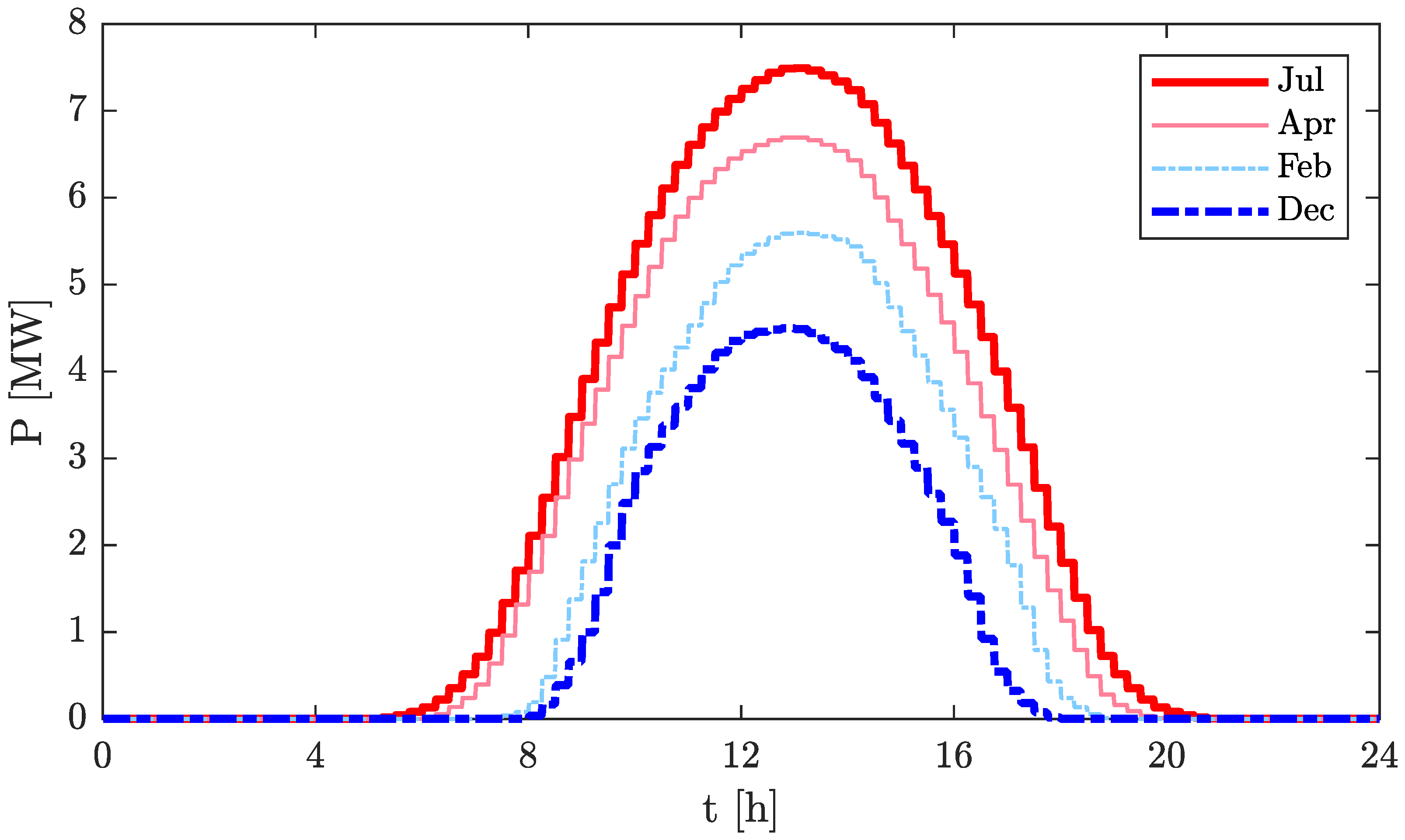
In particular, the numerical model of the PV computes the quarter-hour power production profiles on a mean day of each month starting from the solar irradiance, the temperature, the PV panel characteristics and the ambient temperature. 
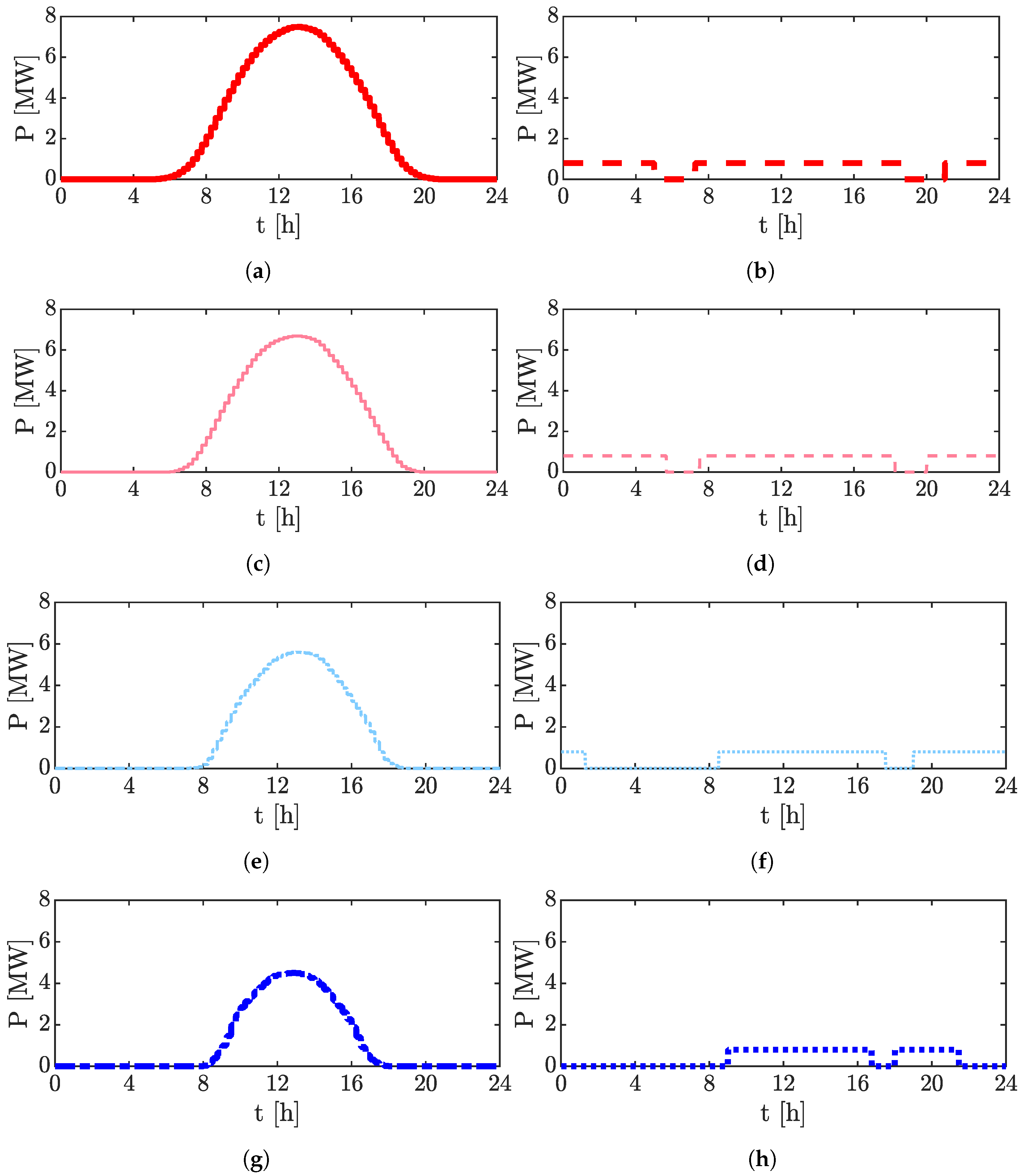
Figure 3 reports the four-month quarter-hour power production profiles. The PV power generation is considered the same for each day of a single month. The estimated profile of each day of each month allows computing both the monthly and the annual mean production of the PV plant. Comparisons between the electricity production estimations and the confidential data provided by the PV owner indicate a mismatch lower than 2% on both monthly and annual bases.
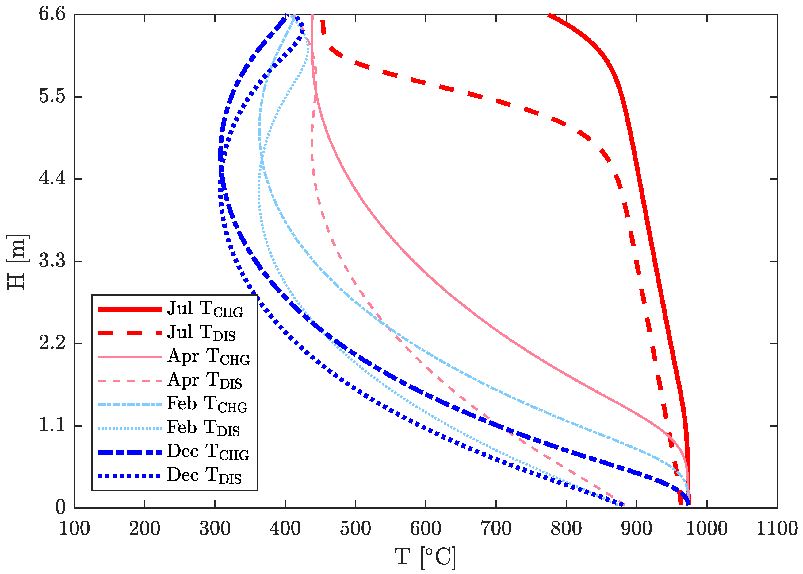
Despite using a monthly average PV production profile, the VPP model is wholly dynamic since the temperature distribution within the I-ESS storage tank varies depending on the quantity of energy stored and restored over the day. As a result, the performance of the VPP is calculated using a yearlong simulation.
Note that the TES temperature profiles—after an adjustment period occurring in the first days of the month (the day-by-day difference of the thermal profiles is caused by the change in the PV production profile at the beginning of each month)—became regular despite the TES tank loss change based on the ambient temperature. In the model, this value changes on an hourly basis. It is also essential to highlight that the simulations cannot perfectly match the real PV production behavior since meteorological variability cannot be considered in a mathematical model. However, the arrangement represents a good starting point to simulate the coupling of the two systems and estimate the potential of storing the PV electricity as sensible heat.
The I-ESS model governing equations are widely detailed in Refs. [12,13]. Compared to Refs. [12,13], the TES mathematical model is updated with the so-called TES-PD model, a TES system numerical model developed in house at the Industrial Engineering Department of the University of Padova by the present research group. The interested reader can refer to Refs. [49,57,58] for a complete description of the model, while in the following, only a quick rundown is given. The tank model behaves according to the following set of Partial Differential Equations (PDE):
ρ f t + ( ρ f v f ) x = 0
( ρ f T f ) t + ( ρ f T f v f ) x = 1 ε α ( T s T f )
( ρ s c p , s T s ) t + x k s , e f f T s x = c p , f 1 ε α ( T f T s ) U i C u ( 1 ε ) ( T s T a m b )
This set of equations consists of the fluid’s mass conservation equation, the fluid energy conservation equation and the solid energy conservation equation. The model’s closure is made by a constitutive expression for the pressure drop and the ideal gas equation of state:
p x = C f β 1 2 ρ f v f 2
p = ρ f r T f
Here t, x and L denote the time, the axial tank coordinate and the length, respectively; ρ f , v f , T f and p are the fluid density, velocity, temperature and thermodynamic pressure. ρ s and T s are the storage material density and temperature. k f and k s , e f f are the fluid and the solid effective thermal conductivity, while c p , f and c p , s are the fluid and the solid specific heat coefficient at constant pressure. ε is the void fraction, T a m b is the ambient temperature and r is the specific gas constant. The α and β coefficients assume different values depending on the storage material geometry. The present case concerns sphere packing, then
α = 6 d 2 N u k f c p , f 1
β = ( 1 ε ) ( d ε ) 1
where d is the particle equivalent diameter. C u ( 1 ε ) 1 denotes the external surface to volume ratio while U i is the overall heat loss coefficient. C u = 4 L 1 when the considered geometry is sphere packing. N u is the Nusselt number and C f is the friction coefficient. The TES-PD model employs a first-order explicit Euler scheme for temporal integration and a first-order generalized upwind finite difference approach for spatial terms. A second-order central approximation based on the method proposed by De Vanna et al. [59] is used for diffusive terms accounting for cell variability of the physical parameters. Such integration strategies are selected based on computational correctness and efficiency. As said, Ref. [49] offers further information concerning boundary conditions, model validation and numerical implementation issues.
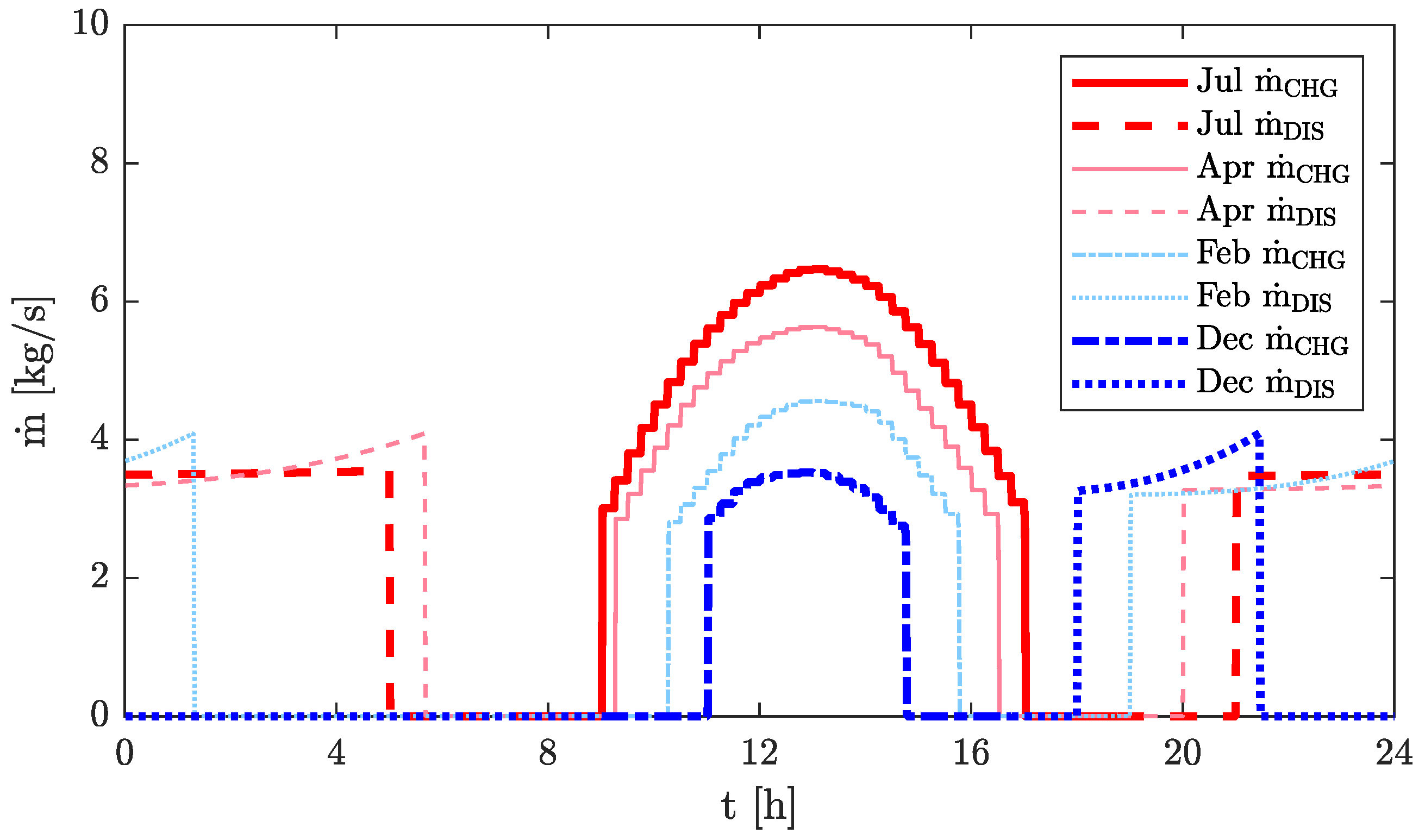
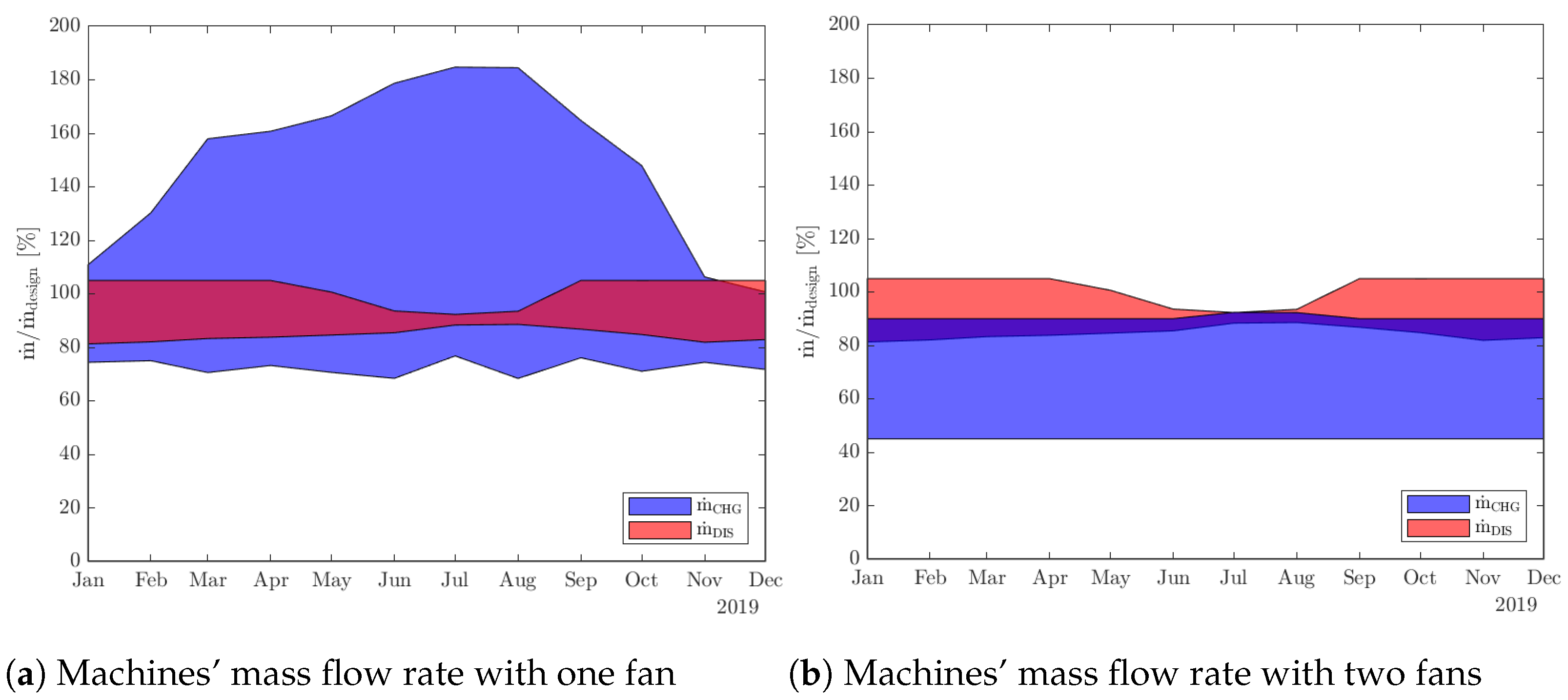
During the charging phase, the PV power availability drives the power profile through a mass flow rate control, which becomes a TES-PD model boundary condition. Because of the operational constraints of each system’s components, not all mass flow rate values are allowed. Thus, multiple fans are employed to reach the mass flow rates necessary for power generation while maintaining an appropriate functioning range. The operational range of turbine mass flow rate is significantly more limited. An approach for meeting these criteria is to impose two mass flow rate constraints (specified on the nominal mass flow rate of the gas turbine used). The first limitation is the minimum mass flow rate during the charging phase, which must be greater than 0.7 · m ˙ d e s i g n . The constant power output P D I S ensures a minimal mass flow rate throughout the discharging phase, but when the temperature of the air outflow from the tank begins to decline, the mass flow rate begins to climb. As a result, a maximum mass flow rate limitation must be imposed, i.e., the mass flow rate must not exceed 1.05 · m ˙ d e s i g n , i.e., 105% of the value for the gas turbine. In both situations, m ˙ d e s i g n is enforced to the gas turbine design mass flow rate. These constraints affect the charging and discharging processes: charging occurs when the plant’s power output surpasses a value that allows the mass flow rate to be greater than the minimum, while discharging occurs when the mass flow rate ensures P D I S exceeds the maximum. The ambient temperature, which is important in thermal heat exchange with the tank’s coating and even indicates the temperature of the inflow air into the system, is selected differently for each month according to meteorological data.
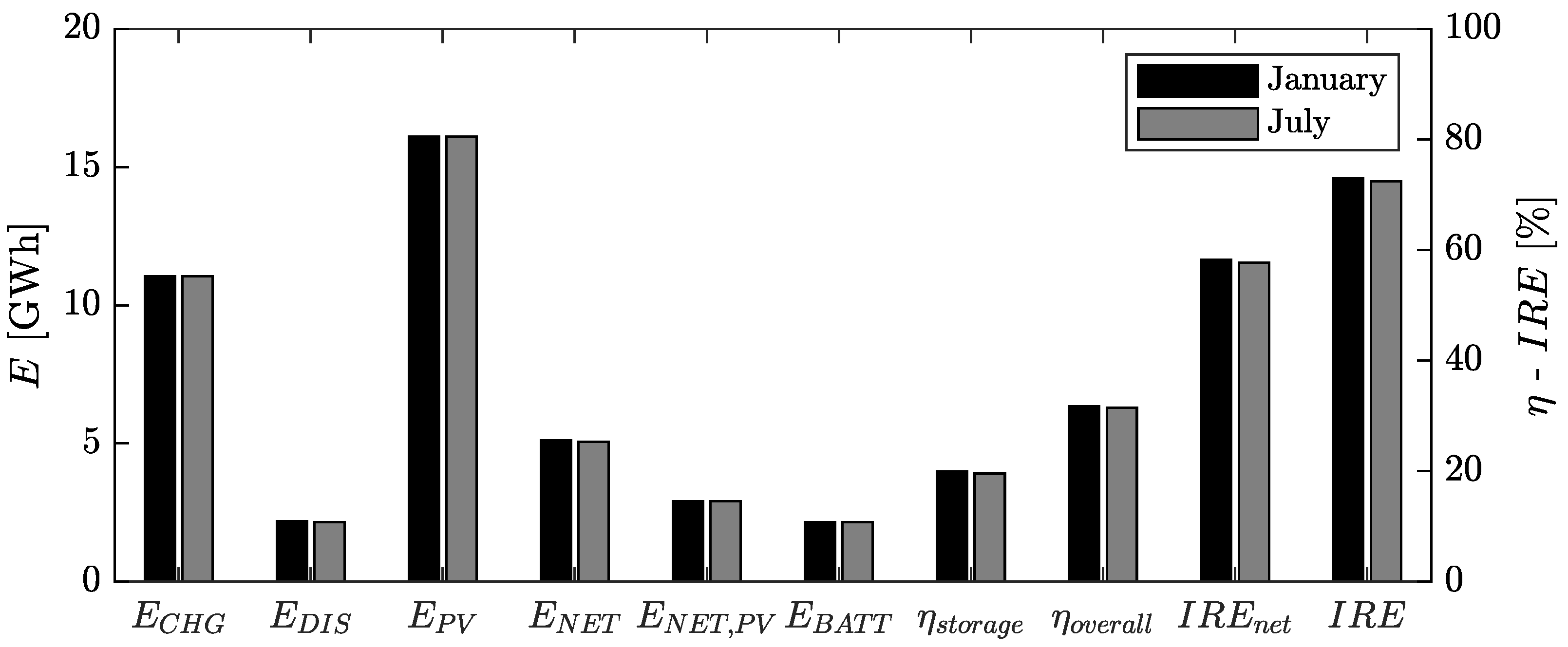
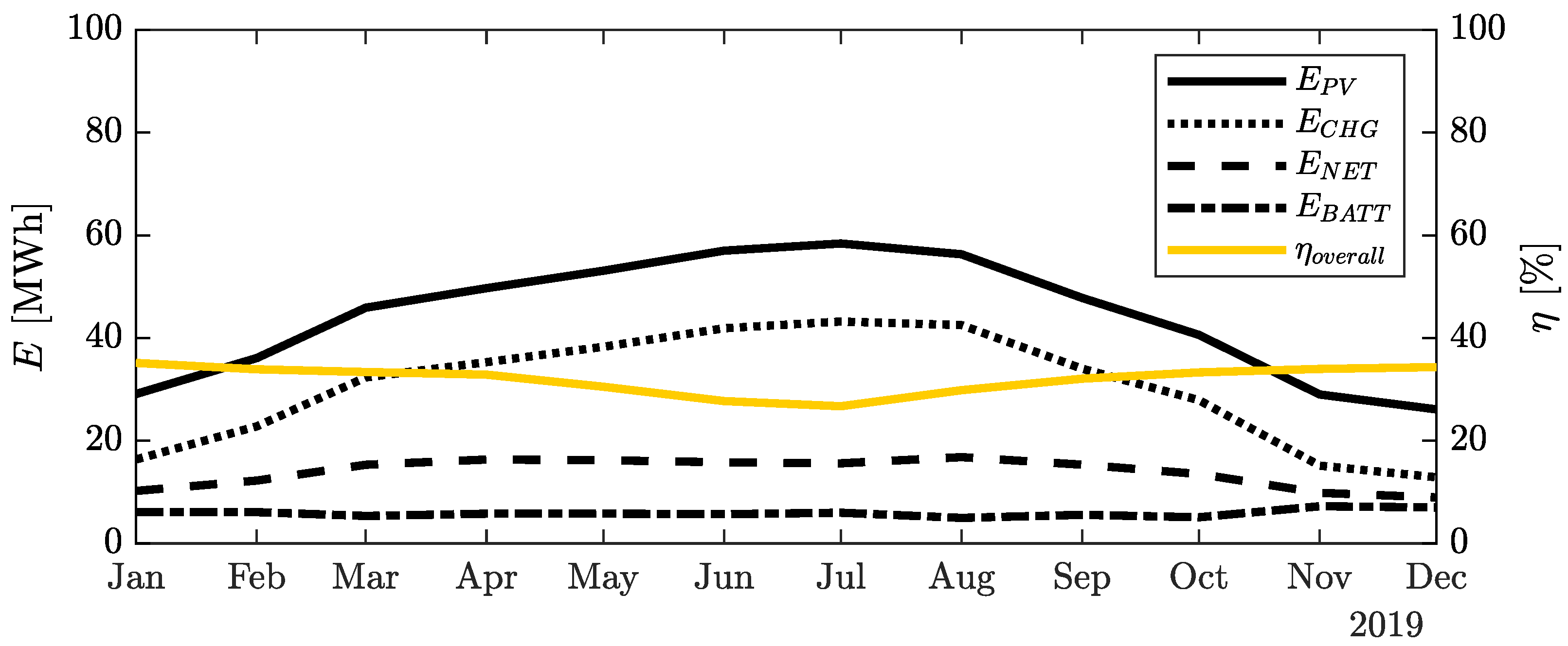
To evaluate the VPP performance, some mathematical identities need to be defined. At first, energy is defined as
E = t P ( τ ) d τ
where P ( τ ) is the time-varying power. E C H G and E D I S denote the total amount of energy involved in the charging and discharging processes, respectively, while E P V is the total production of the PV power plant and E N E T is the total amount of energy injected into the grid by the VPP plant. E N E T , P V is the total amount of energy produced by the PV and directly injected into the grid. Thus, E N E T , P V is related to E N E T and E D I S as
E N E T , P V = E N E T E D I S i f P N E T > E N E T , P V
E B A T T is energy stored in the battery pack. Concerning performance parameters, η s t o r a g e is the storage efficiency
η s t o r a g e = E D I S E C H G
while η o v e r a l l is the overall VPP efficiency, so the following equation holds
η o v e r a l l = E N E T E P V
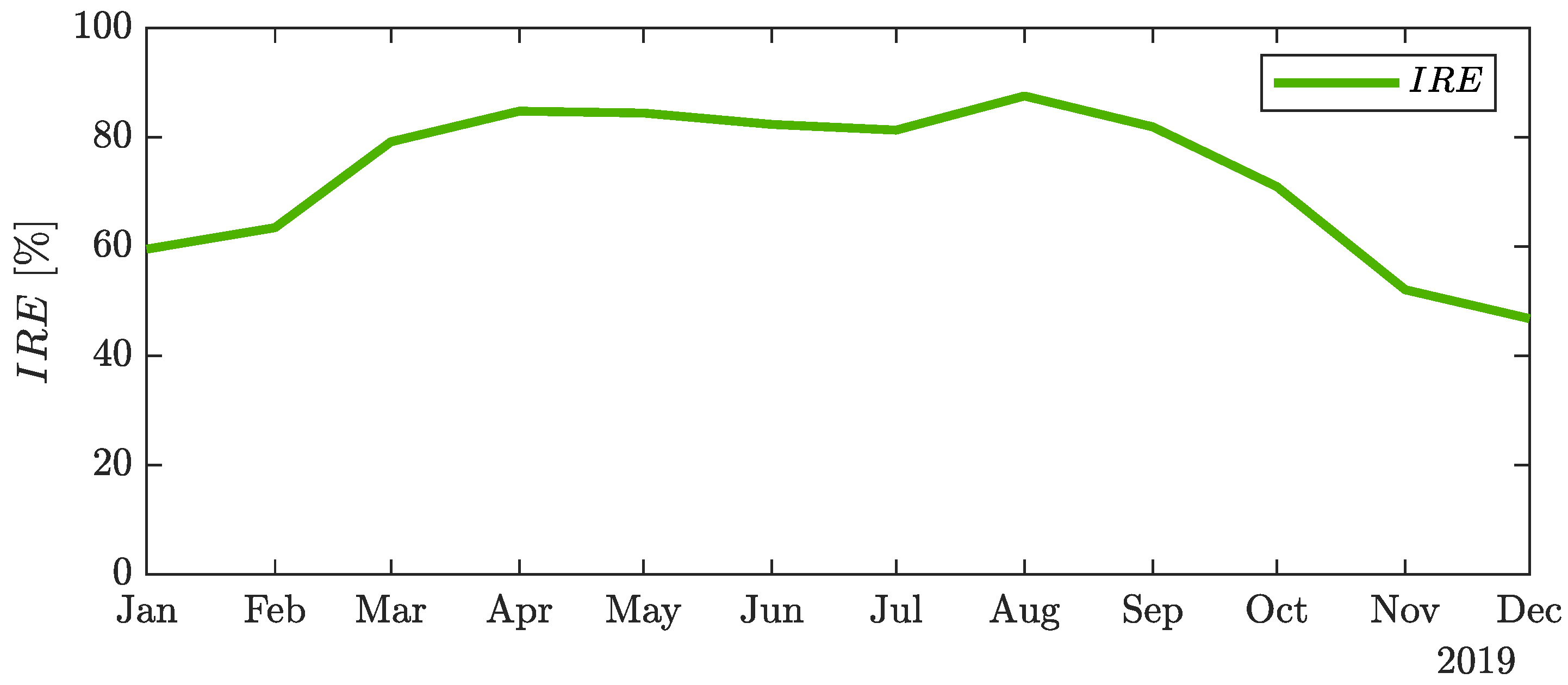
In addition, some regularity indices are also defined. Thus, the net regularity index, I R E n e t ,
I R E n e t = t f ( τ ) d τ Δ t , f ( τ ) = 1 , if P D I S = 0.8 MW 0 , if P D I S 0.8 MW
represents the percentage of the hours of the year in which the VPP provides constant power to the grid. Its value is computed according to the following equation: The regularity index, I R E , instead,
I R E = t f ( τ ) d τ Δ t , f ( τ ) = 1 , if P D I S 0.8 MW 0 , if P D I S < 0.8 MW
denotes the percentage of the hours of the year in which the VPP provides the constant power to the grid plus the hours that the energy is stored in the battery pack.

3. Results and Discussion

3.1. Influence of Plant Starting Month

As a first step in delineating the VPP characteristics and in light of the variable and intermittent nature of solar energy, it is necessary to investigate whether the annual performance of the VPP is affected by the period in which the plant begins to operate, as well as the charging time from empty to fully charged based on the PV profile. For that purpose, the authors examined VPP performance when it began operations in January or July. These are the months with the lowest and highest solar output, respectively. Given that the tank’s initial temperature corresponds to the ambient temperature, the TES requires five or ten days to reach the fully-charged state, depending on whether the PV production profile starts. The analysis is carried out with the I-ESS fully charged when it begins operation and the plant is set in charging mode.
As expected, solar output affected the I-ESS storage’s first-charge time, influencing the system’s annual performance. The only difference between the two beginning points is the recovered energy, which is somewhat more significant if the plant begins operations in January. In actuality, instead of 5.067 GWh, the total quantity of energy sent into the electric system in a year is 5.106 GWh. Because more energy is delivered to the grid, the E N E T directly impacts overall efficiency. However, we must examine the TES behavior during the January and July operations to appreciate this little difference. We see that having a fully charged TES in January is more important than in July because solar irradiation and PV output are lower in the winter; a TES with more stored energy assures a little more production. In contrast, if operations begin with a fully charged TES in July, the average TES internal temperature after six months is lower than that of the fully charged state (965 °C). So, during the winter, productivity is lower and on an annual basis, it is 0.8% lower. Obviously, these small and negligible deviations become zero during the second year of continuous operations, as shown by a five-year simulation. More quantitative information concerning discrepancies between January and July operation starts are reported in Figure 4.
It deserves to be noted that in all of the examples presented in this investigation, the management plan does not address the potential of charging the TES with an external source entirely or partly during the annual operation. So, the TES starts with a fully charged battery, but the TES is recharged exclusively using PV surplus energy. Since the difference in starting the plant operation in January versus July is negligible (less than 0.8%), the following results referred to the case in which the VPP starts the operation on 1 January with a TES tank at a uniform temperature equal to 965 °C because the first-charge had already been made. Furthermore, as a starting condition, the amount of energy required to charge the I-ESS tank is not incorporated in the yearly performance calculation.

3.2. Temperature and Mass Flow Rate Trends in TES Tank

Before concentrating on the VPP’s overall performance, given the PV source’s significant fluctuation throughout the year, it is worthwhile to go further into the analysis of both the temperature trend inside the TES tank and the machine mass flow rate to understand the I-ESS behavior better. The temperature distribution within the tank after the charging and discharging operations is reported in Figure 5. From the reported trends, it is clear that during the summer, the storage tank is almost fully charged. Conversely, in the winter, the temperature of some tank sections becomes lower than the air temperature after the compression phase. Here, it is worth mentioning that, among the various tank models available in the literature [16,18,54] this fact is captured only by the TES-PD model, which accounts for the heat exchange with the external environment layer-by-layer as well as the conductive effects within the layers. When the amount of energy to be stored is low, some tank sections are not active; therefore, heat exchange via the coating becomes much more critical. As a result, we can see that during the colder and lower irradiance months, PV generation may partly recharge the TES, but not efficiently. Thus, it may be advantageous to arrange a TES full-charge utilizing an external source of power (e.g., excess energy produced by wind turbines). This extra full charge may raise the tank mean temperature and, as a result, improve the VPP’s effectiveness. It should be noted that the storage’s utilization may be altered with various control tactics, for example, a shorter discharging phase; hence, future research will focus on optimizing the TES temperature profile under different VPP management strategies.
The TES state of charge, which depends on the temperature profiles inside the tank itself, also affected the I-ESS machines’ behavior. Figure 6 depicts the evolution of the mass flow rate during the charging and discharging process to guarantee the correct power consumption/generation for four representative months.
The mass flow rate trends on the mean day of the month provide information on the system’s operating control. During the stabilized cycle (end of the month) in July and other hot months, the airflow rate during the discharging phase is practically constant. During the cold months, it increases until reaching the maximum value, which is due to the tank outlet’s air temperature drop. To maintain the discharging power P D I S at the fixed value and avoid grid issues, the control strategy forces the air flow rate to increase. So, to avoid this operation, it can be helpful to plan a full-charge cycle with an external source during the winter months. This procedure can stabilize the TES temperature and improve the machines’ performance. In contrast, the mass flow rate profile during the charge depends on the power made available by the PV plant. So, with PV production being smaller during winter months, the flow rate used to charge the system is lower compared to sunny months.
Figure 7 depicts the trends of both charging power and that delivered to the grid by the VPP for the mean day of the four most representative months. During the charge and the discharge, the power supply to the grid is constant and fixed equal to 800 kW and named P N E T . The value is that able to preserve the grid stability according to the grid manager. During the charge and the discharge transition, the power fed into the grid varies from zero to a maximum value, beyond which the charging phase of the tank could start (Figure 8). Similarly, at the end of the charging process, the power falls from a maximum value to zero before the discharging phase begins. Since the power in these periods is not enough to charge the TES or be delivered to the grid, storing this energy in a battery pack is convenient. Such a solution avoids energy losses and guarantees a power source to start the I-ESS power train during the delivery mode.
Not that the need to store energy in an auxiliary system is strictly related to the operation ranges of the components. In this regard, Figure 9a shows the mass flow rate range in the charging and discharging phase, expressed as a percentage of the machine’s design mass flow rate. For the charge phase, the latter is the single fan design flow rate while, for the discharge, it is represented by the gas turbine sort. The minimum in the charging phase concerns both the mass flow rate lower limit for the fan and the flow state into the storage tank. The Reynolds number of particles at the minimum flow rate is not below 50 to guarantee the correct heat exchange between the fluid and the storage solid. Furthermore, the Biot number never exceeds the value of 0.1, i.e., a threshold that, once exceeded, would cause the one-dimensional model of the tank not to be very reliable. Due to the wide variability of the mass flow rate of the fan during the charging phase, Figure 9b shows the mass flow rate values, considering the possibility of using multiple fans for the charging phase. The choice is to adopt two fans, enabling the system to operate even in high power peaks. Indeed the mass flow rate for the single fan remains below 95% with this setup.

3.3. VPP Grid Output and Performance

Figure 10 depicts the PV power profile and the power profile fed to the grid on the mean day of July, April, February and December. The input profile is the same on all days of the month, while the power delivered by the VPP to the grid is almost identical on all days of the specified month. Thus, the power profile for the mean day of each month is reported. It is easy to see that the discharge phase of the storage tank is continuous between April and July. The control logic does not approach the mass flow rate limit during these months, indicating that the storage tank has additional discharge potential. The excess energy saving throughout the summer months boosts energy availability in the initial days of the next month or allows for more regular operation after low radiation days during the same time.
It should be noted that the timing of storage discharges, particularly during the winter months, is a decision made by the grid operator. In fact, the storage is released from 7 p.m. to 2 a.m. in Figure 10f. Figure 11 shows how the control approach may be simply adjusted. Rather than discharging the TES between 7 p.m. and 2 a.m., the system might provide 800 kW between 7 p.m. and 10 p.m. This is because these are peak hours in Italy. Then it is turned off and reactivated between 6 and 7 a.m. The TES is not totally drained when the VPP is managed in this manner and some of the energy stored may be utilized in the following manner. This management method also enables economic power distribution advantages to the grid. Indeed, since electrical energy prices fluctuate daily, it may be advantageous to manage the discharging phase during the cold months to cover the precise times defined by the highest selling price and optimize plant income. Indeed, such inquiries are not part of the current study but are natural comments on the actual standings and will undoubtedly be studied more thoroughly in future research.
After discussing the power profiles, it is important to highlight how the dynamic nature of the I-ESS affects the VPP performance. Figure 12 shows the monthly mean performance indexes of the VPP. As can be seen, energy trends of the system’s components (i.e., PV system, batteries, tanks, etc.) show very different behavior over the year. However, the overall efficiency of the production and storage system is almost constant over the 12 months, fluctuating in a range between 35 and 40%.
The study’s most noteworthy finding is the regularity index, I R E . The latter for each month shows what percentage of total hours the power equals the target distribution.
August is the most consistent month, with almost 87% of regular power feeding hours (see, Figure 13). In chilly months, regularity is not well respected; the system’s activity convenience should be reviewed at these times. However, since these findings are for an average day, the backup storage system might be critical in these cases. These indices have a maximum value tied to the system’s control logic description. As soon as PV power is available, the switch from tank discharge to electricity provided directly by the PV system begins. An alternative logic may be to drain the tank until the power available is less than P D I S : in this scenario, achieving an I R E of 100% is conceivable. However, there would be two additional power jumps, not to mention the possibility of a transient during the transfer of operating modes.

4. Conclusions

The widespread use of variable and unpredictable RESs, such as wind and solar, in the energy mix is seen as both a critical component of accelerating the transition to a decarbonized and sustainable energy system and a source of concern due to issues associated with managing high fluctuating power production. For these reasons, various researchers are working to develop storage technologies that can match energy supply and demand without experiencing large power swings, which may cause management and control issues as well as device malfunctions. Thus, because of its predicted dependability, TES systems for electrical applications are gaining much attention. In this study, the following goals are reached:
  • For the first time, the authors’ patented and well-established TES plant, the so-called I-ESS, is evaluated in conjunction with an RES plant. The I-ESS unit, in particular, is linked to a 10 MWp PV plant, establishing a VPP and seeking to deliver a consistent power profile to the grid.
  • It is found that the proposed VPP plant effectively smoothes the PV peak and manages the power supply.
  • Novel metrics are proposed to evaluate the VPP supply regularity quantitatively and, in particular, the I R E and the I R E n e t indexes are proposed. These denote the ratio between regular hours of power provided to the grid plus the energy stored in the backup unit and the total number of hours in a year, which is designed to offer information on power regularity.
  • Analyses reveal that the VPP regularity is relatively high in terms of PV output, ranging from a low of 50% in December to a high of 87% in August.
Based on these findings, the proposed VPP is, therefore, very promising in terms of regularizing the power generated by PV and revamping in-decommissioning gas plants or partly existing facilities with subtle changes and costs. Obviously, in future works, other management strategies can be tested, including economic issues or different market scenarios. Moreover, comparisons among the proposal and configurations using a unique storage unit, battery, PTES, gravity energy storage, etc., can be helpful in further investigating the technical and economic viability of the proposed VPP arrangement.

Author Contributions

Conceptualization, A.B. and F.D.V.; methodology, A.B., F.D.V. and A.S.; validation, A.B. and F.D.V.; formal analysis, A.B. and F.D.V.; writing—original draft preparation, A.B. and F.D.V.; writing—review and editing, A.B., F.D.V. and A.S. All authors have read and agreed to the published version of the manuscript.

Funding

This research received no external funding.

Institutional Review Board Statement

Not applicable.

Informed Consent Statement

Not applicable.

Data Availability Statement

Not applicable.

Conflicts of Interest

The authors declare no conflict of interest.

Abbreviations

The following abbreviations are used in this manuscript:
COMPCompressor
CSPConcentrating Solar Power
EGDEuropean Grean Deal
EHElectric Heater
EUEuropean Union
HXHeat Exchanger
I-ESSIntegrated Energy Storage System
MElectric Motor
MGElectric Motor/Generator
PTESPumped Thermal Energy Storage
PVPhotoVoltaic
VPPVirtual Power Plant
RESRenewable Energy Source
TESThermal Energy Storage
TURBTurbine
USAUnited States of America

References

  1. The United Nations Framework Convention on Climate Change. The Kyoto Protocol. UNFCCC Website. 1997. Available online: http://unfccc.int/kyoto_protocol/items/2830.php (accessed on 10 September 2022).
  2. The United Nations Framework Convention on Climate Change. The Paris Agreement. UNFCCC Website. 2015. Available online: https://unfccc.int/documents/184656 (accessed on 10 September 2022).
  3. European Parliament and of the Council. Directive 2009/28/EC of the European Parliament and of the Council of 23 April 2009 on the promotion of the use of energy from renewable sources and amending and subsequently repealing Directives 2001/77/EC and 2003/30/EC. Off. J. Eur. Union 2009, 5. Available online: https://eur-lex.europa.eu/legal-content/en/ALL/?uri=CELEX%3A32009L0028 (accessed on 10 September 2022).
  4. The European Commission. The EU 2030 Climate and Energy Framework. Off. J. Eur. Union 2014. Available online: https://ec.europa.eu/clima/eu-action/climate-strategies-targets/2030-climate-energy-framework_it (accessed on 10 September 2022).
  5. The European Commission. Roadmap 2050: Roadmap for moving to a competitive low-carbon economy in 2050. Off. J. Eur. Union 2011. Available online: https://www.roadmap2050.eu/ (accessed on 10 September 2022).
  6. The European Parliament. EU Responses to Climate Change. Official Website of the European Parliament, 2022. Available online: https://www.europarl.europa.eu/news/en/headlines/society/20180703STO07129/eu-responses-to-climate-change (accessed on 10 September 2022).
  7. The European Commission. The European Green Deal. Off. J. Eur. Union 2020. Available online: https://www.europarl.europa.eu/news/en/headlines/society/20200618STO81513/green-deal-key-to-a-climate-neutral-and-sustainable-eu (accessed on 10 September 2022).
  8. Ministero dello Sviluppo Economico. Piano Nazionale Integrato per l’Energia e il Clima 2030. Gazz. Uff. Della Repubb. Ital. 2020. Available online: https://www.mise.gov.it/index.php/it/energia/energia-e-clima-2030 (accessed on 10 September 2022).
  9. GSE—Gestore dei Servizi Energetici S.p.A. Rapporto Statistico 2020 Energia e Fonti Rinnovabili in Italia al 2020. GSE Official Website. 2020. Available online: https://www.gse.it/documenti_site/Documenti%20GSE/Rapporti%20statistici/Rapporto%20Statistico%20GSE%20-%20FER%202020.pdf (accessed on 10 September 2022).
  10. Mbah, R.E.; Wasum, D.F. Russian-Ukraine 2022 War: A review of the economic impact of Russian-Ukraine crisis on the USA, UK, Canada and Europe. Adv. Soc. Sci. Res. J. 2022, 9, 144–153. [Google Scholar] [CrossRef]
  11. The European Commission. RePowerEU: A plan to rapidly reduce dependence on Russian fossil fuels and fast forward the green transition. Off. J. Eur. Union 2022. Available online: https://eur-lex.europa.eu/resource.html?uri=cellar:fc930f14-d7ae-11ec-a95f-01aa75ed71a1.0001.02/DOC_1&format=PDF (accessed on 10 September 2022).
  12. Benato, A.; Stoppato, A. Energy and cost analysis of an Air Cycle used as prime mover of a Thermal Electricity Storage. J. Energy Storage 2018, 17, 29–46. [Google Scholar] [CrossRef]
  13. Benato, A.; Stoppato, A. Integrated thermal electricity storage system: Energetic and cost performance. Energy Convers. Manag. 2019, 197, 111833. [Google Scholar] [CrossRef]
  14. Desrues, T.; Ruer, J.; Marty, P.; Fourmigue, J.F. A thermal energy storage process for large scale electric applications. Appl. Therm. Eng. 2010, 30, 425–432. [Google Scholar] [CrossRef] [Green Version]
  15. Howes, J. Concept and development of a pumped heat electricity storage device. Proc. IEEE 2011, 100, 493–503. [Google Scholar] [CrossRef]
  16. White, A.J. Loss analysis of thermal reservoirs for electrical energy storage schemes. Appl. Energy 2011, 88, 4150–4159. [Google Scholar] [CrossRef] [Green Version]
  17. White, A.; Parks, G.; Markides, C.N. Thermodynamic analysis of pumped thermal electricity storage. Appl. Therm. Eng. 2013, 53, 291–298. [Google Scholar] [CrossRef] [Green Version]
  18. White, A.; McTigue, J.; Markides, C. Wave propagation and thermodynamic losses in packed-bed thermal reservoirs for energy storage. Appl. Energy 2014, 130, 648–657. [Google Scholar] [CrossRef] [Green Version]
  19. McTigue, J.D.; White, A.J.; Markides, C.N. Parametric studies and optimisation of pumped thermal electricity storage. Appl. Energy 2015, 137, 800–811. [Google Scholar] [CrossRef] [Green Version]
  20. White, A.J.; McTigue, J.D.; Markides, C.N. Analysis and optimisation of packed-bed thermal reservoirs for electricity storage applications. Proc. Inst. Mech. Eng. Part J. Power Energy 2016, 230, 739–754. [Google Scholar] [CrossRef]
  21. McTigue, J.; White, A. A comparison of radial-flow and axial-flow packed beds for thermal energy storage. Appl. Energy 2018, 227, 533–541. [Google Scholar] [CrossRef]
  22. Thess, A. Thermodynamic efficiency of pumped heat electricity storage. Phys. Rev. Lett. 2013, 111, 110602. [Google Scholar] [CrossRef] [Green Version]
  23. Ni, F.; Caram, H.S. Analysis of pumped heat electricity storage process using exponential matrix solutions. Appl. Therm. Eng. 2015, 84, 34–44. [Google Scholar] [CrossRef]
  24. Guo, J.; Cai, L.; Chen, J.; Zhou, Y. Performance evaluation and parametric choice criteria of a Brayton pumped thermal electricity storage system. Energy 2016, 113, 693–701. [Google Scholar] [CrossRef]
  25. Abarr, M.; Hertzberg, J.; Montoya, L.D. Pumped Thermal Energy Storage and Bottoming System Part B: Sensitivity analysis and baseline performance. Energy 2017, 119, 601–611. [Google Scholar] [CrossRef]
  26. Abarr, M.; Geels, B.; Hertzberg, J.; Montoya, L.D. Pumped thermal energy storage and bottoming system part A: Concept and model. Energy 2017, 120, 320–331. [Google Scholar] [CrossRef]
  27. Benato, A. Performance and cost evaluation of an innovative Pumped Thermal Electricity Storage power system. Energy 2017, 138, 419–436. [Google Scholar] [CrossRef]
  28. Benato, A.; Stoppato, A. Energy and cost analysis of a new packed bed pumped thermal electricity storage unit. J. Energy Resour. Technol. 2018, 140. [Google Scholar] [CrossRef]
  29. Wang, L.; Lin, X.; Chai, L.; Peng, L.; Yu, D.; Liu, J.; Chen, H. Unbalanced mass flow rate of packed bed thermal energy storage and its influence on the Joule-Brayton based Pumped Thermal Electricity Storage. Energy Convers. Manag. 2019, 185, 593–602. [Google Scholar] [CrossRef]
  30. Wang, L.; Lin, X.; Zhang, H.; Peng, L.; Chen, H. Brayton-cycle-based pumped heat electricity storage with innovative operation mode of thermal energy storage array. Appl. Energy 2021, 291, 116821. [Google Scholar] [CrossRef]
  31. Zhao, Y.; Song, J.; Liu, M.; Zhao, Y.; Olympios, A.V.; Sapin, P.; Yan, J.; Markides, C.N. Thermo-economic assessments of pumped-thermal electricity storage systems employing sensible heat storage materials. Renew. Energy 2022, 186, 431–456. [Google Scholar] [CrossRef]
  32. Albert, M.; Ma, Z.; Bao, H.; Roskilly, A.P. Operation and performance of Brayton Pumped Thermal Energy Storage with additional latent storage. Appl. Energy 2022, 312, 118700. [Google Scholar] [CrossRef]
  33. Bahzad, H.; Fennell, P.; Shah, N.; Hallett, J.; Ali, N. Techno-economic assessment for a pumped thermal energy storage integrated with open cycle gas turbine and chemical looping technology. Energy Convers. Manag. 2022, 255, 115332. [Google Scholar] [CrossRef]
  34. Zhang, H.; Wang, L.; Lin, X.; Chen, H. Technical and economic analysis of Brayton-cycle-based pumped thermal electricity storage systems with direct and indirect thermal energy storage. Energy 2022, 239, 121966. [Google Scholar] [CrossRef]
  35. Wang, L.; Lin, X.; Zhang, H.; Peng, L.; Zhang, X.; Chen, H. Analytic optimization of Joule–Brayton cycle-based pumped thermal electricity storage system. J. Energy Storage 2022, 47, 103663. [Google Scholar] [CrossRef]
  36. Benato, A.; Stoppato, A.; Mirandola, A. State-of-the-art and future development of sensible heat thermal electricity storage systems. Int. J. Heat Technol. 2017, 35, S244–S251. [Google Scholar] [CrossRef]
  37. Benato, A.; Stoppato, A. Pumped thermal electricity storage: A technology overview. Therm. Sci. Eng. Prog. 2018, 6, 301–315. [Google Scholar] [CrossRef]
  38. Smallbone, A.; Jülch, V.; Wardle, R.; Roskilly, A.P. Levelised Cost of Storage for Pumped Heat Energy Storage in comparison with other energy storage technologies. Energy Convers. Manag. 2017, 152, 221–228. [Google Scholar] [CrossRef]
  39. Dumont, O.; Frate, G.F.; Pillai, A.; Lecompte, S.; Lemort, V.; De paepe, M. Carnot battery technology: A state-of-the-art review. J. Energy Storage 2020, 32, 101756. [Google Scholar] [CrossRef]
  40. Novotny, V.; Basta, V.; Smola, P.; Spale, J. Review of Carnot Battery Technology Commercial Development. Energies 2022, 15, 647. [Google Scholar] [CrossRef]
  41. Liang, T.; Vecchi, A.; Knobloch, K.; Sciacovelli, A.; Engelbrecht, K.; Li, Y.; Ding, Y. Key components for Carnot Battery: Technology review, technical barriers and selection criteria. Renew. Sustain. Energy Rev. 2022, 163, 112478. [Google Scholar] [CrossRef]
  42. Petrollese, M.; Cascetta, M.; Tola, V.; Cocco, D.; Cau, G. Pumped thermal energy storage systems integrated with a concentrating solar power section: Conceptual design and performance evaluation. Energy 2022, 247, 123516. [Google Scholar] [CrossRef]
  43. Miao, M.; Wu, Z.; Lou, S.; Wang, Y. Research on optimizing operation of hybrid PV power and pumped hydro storage system. Energy Procedia 2017, 118, 110–118. [Google Scholar] [CrossRef]
  44. Cavazzini, G.; Benato, A.; Pavesi, G.; Ardizzon, G. Techno-economic benefits deriving from optimal scheduling of a Virtual Power Plant: Pumped hydro combined with wind farms. J. Energy Storage 2021, 37, 102461. [Google Scholar] [CrossRef]
  45. Björk, J.; Johansson, K.H.; Dörfler, F. Dynamic Virtual Power Plant design for fast frequency reserves: Coordinating hydro and wind. IEEE Trans. Control. Netw. Syst. 2022. [Google Scholar] [CrossRef]
  46. Abbasi, M.H.; Taki, M.; Rajabi, A.; Li, L.; Zhang, J. Coordinated operation of electric vehicle charging and wind power generation as a Virtual Power Plant: A multi-stage risk constrained approach. Appl. Energy 2019, 239, 1294–1307. [Google Scholar] [CrossRef]
  47. Wang, W.; Chen, P.; Zeng, D.; Liu, J. Electric vehicle fleet integration in a Virtual Power Plant with large-scale wind power. IEEE Trans. Ind. Appl. 2020, 56, 5924–5931. [Google Scholar] [CrossRef]
  48. Benato, A.; Pezzuolo, A.; Stoppato, A. Impianto e Metodo per l’Accumulo di Energia e la Successiva Produzione di Energia Elettrica 2016. Italian Patent Reference Number: 102016000079091, 5 November 2019. [Google Scholar]
  49. Benato, A.; De Vanna, F.; Gallo, E.; Stoppato, A.; Cavazzini, G. TES-PD: A Fast and Reliable Numerical Model to Predict the Performance of Thermal Reservoir for Electricity Energy Storage Units. Fluids 2021, 6, 256. [Google Scholar] [CrossRef]
  50. Singh, H.; Saini, R.; Saini, J. A review on packed bed solar energy storage systems. Renew. Sustain. Energy Rev. 2010, 14, 1059–1069. [Google Scholar] [CrossRef]
  51. Hesse, H.C.; Schimpe, M.; Kucevic, D.; Jossen, A. Lithium-ion battery storage for the grid—A review of stationary battery storage system design tailored for applications in modern power grids. Energies 2017, 10, 2107. [Google Scholar] [CrossRef]
  52. Atlas, G.S. Global Solar Atlas 2.0, a Free, Web-Based Application is Developed and Operated by the Company Solargis s.r.o. on behalf of theWorld Bank Group, Utilizing Solargis Data, with Funding Provided by the Energy Sector Management Assistance Program (esmap). Web Source. Available online: https://globalsolaratlas.info (accessed on 10 September 2022).
  53. Meteo, I. Il Meteo. Web Source. Available online: https://www.ilmeteo.it/portale/archivio-meteo/ (accessed on 10 September 2022).
  54. Singh, R.; Saini, R.; Saini, J. Simulated performance of packed bed solar energy storage system having storage material elements of large size—Part I. Open Fuels Energy Sci. J. 2008, 1. [Google Scholar] [CrossRef] [Green Version]
  55. Moler, C. MATLAB. 2021. Available online: https://it.mathworks.com/ (accessed on 10 September 2022).
  56. Bell, I.H.; Wronski, J.; Quoilin, S.; Lemort, V. Pure and pseudo-pure fluid thermophysical property evaluation and the open-source thermophysical property library CoolProp. Ind. Eng. Chem. Res. 2014, 53, 2498–2508. [Google Scholar] [CrossRef] [Green Version]
  57. Benato, A.; De Vanna, F.; Stoppato, A.; Gallo, E. Systematic numerical investigation of a high temperature packed bed for energy storage applications. In Proceedings of the ECOS 2021—the 34th International Conference on Efficiency, Cost, Optimization, Simulation and Environmental Impact of Energy Systems, Taormina, Italy, 27 June–2 July 2021. [Google Scholar]
  58. Benato, A.; De Vanna, F.; Gallo, E.; Stoppato, A. Thermal Energy Storage System integrating into a PV facility. In Proceedings of the ECOS 2022—the 35th International Conference on Efficiency, Cost, Optimization, Simulation and Environmental Impact of Energy Systems, Copenhagen, Denmark, 3–7 July 2022. [Google Scholar]
  59. De Vanna, F.; Benato, A.; Picano, F.; Benini, E. High-order conservative formulation of viscous terms for variable viscosity flows. Acta Mech. 2021, 232, 2115–2133. [Google Scholar] [CrossRef]
Figure 1. The Integrated Energy Storage System plant scheme.
Energies 15 09521 g001
Figure 2. The Virtual Power Plant layout and its interface with the electric grid.
Energies 15 09521 g002
Figure 3. The quarter-hour power production profile derives from an energy data piecewise shape-preserving cubic polynomial interpolation for the average day of each month. From the interpolation, a quarter-hour based power distribution is derived by averaging power every fifteen minutes.
Energies 15 09521 g003
Figure 4. Graphical comparison of overall energy and efficiency starting from January or July.
Energies 15 09521 g004
Figure 5. Temperature profiles inside the storage tank. A single profile denotes the temperature distribution of the selected month at the end of the charging and discharging process of the mean day of the month.
Energies 15 09521 g005
Figure 6. The trends show the evolution of the mass flow rate during the charging and discharging process to guarantee the correct power consumption/generation. The graph shows the mass flow rate during the charging and discharging process on a mean day of of July, April, February and December.
Energies 15 09521 g006
Figure 7. Power trends during the charging and discharging process on the mean day of the months. P C H G denotes the power trend during the charging process, i.e., the PV power consumption by the fans and the electrical heater to charge the storage tank. P N E T is the trend of total power fed to the network in a daily operation.
Energies 15 09521 g007
Figure 8. Amount of energy stored in the additional storage capacity (battery pack).
Energies 15 09521 g008
Figure 9. Mass flow rate ranges for each month. The values are normalised with the design mass flow rate which is 3.9 kg/s for the discharging phase and 3.5 kg/s for the charging phase (more representative for the fans). The area between maximum and minimum values shows possible mass flow rate values during the system operation.
Energies 15 09521 g009
Figure 10. Average PV power profile availability and stable power feed to the grid representations; (a) PV power production in July; (b) Network power trend in July; (c) PV power production in April; (d) Network power trend in April; (e) PV power production in February; (f) Network power trend in February; (g) PV power production in December; (h) Network power trend in December.
Energies 15 09521 g010
Figure 11. Power trends during the charging and discharging process from the mean day of February. Starting from the stabilised condition (mean day of the month), in an extra day, the discharge occurs from 6 a.m. to the charging phase’s start and from 7 p.m. to 10 p.m. This shows the high flexibility in shifting the power supply to the network. The energy available from the storage is not completely exploited in this case because of the charging phase’s start.
Energies 15 09521 g011
Figure 12. Monthly mean energy trends and overall efficiency.
Energies 15 09521 g012
Figure 13. Graphical trend of monthly regularity indexes.
Energies 15 09521 g013
Publisher’s Note: MDPI stays neutral with regard to jurisdictional claims in published maps and institutional affiliations.

