Advanced Spatial and Technological Aggregation Scheme for Energy System Models

Abstract

Energy system models that consider variable renewable energy sources (VRESs) are computationally complex. The greater spatial scope and level of detail entailed in the models exacerbates complexity. As a complexity-reduction approach, this paper considers the simultaneous spatial and technological aggregation of energy system models. To that end, a novel two-step aggregation scheme is introduced. First, model regions are spatially aggregated to obtain a reduced region set. The aggregation is based on model parameters such as VRES time series, capacities, etc. In addition, spatial contiguity of regions is considered. Next, technological aggregation is performed on each VRES, in each region, based on their time series. The aggregations’ impact on accuracy and complexity of a cost-optimal, European energy system model is analyzed. The model is aggregated to obtain different combinations of numbers of regions and VRES types. Results are benchmarked against an initial resolution of 96 regions, with 68 VRES types in each. System cost deviates significantly when lower numbers of regions and/or VRES types are considered. As spatial and technological resolutions increase, the cost fluctuates initially and stabilizes eventually, approaching the benchmark. Optimal combination is determined based on an acceptable cost deviation of <5% and the point of stabilization. A total of 33 regions with 38 VRES types in each is deemed optimal. Here, the cost is underestimated by $4.42\%$, but the run time is reduced by $92.95\%$.

1. Introduction

1.1. Background: Spatiotemporal Energy System Optimization Models

In the light of international agreements to reduce greenhouse gas (GHG) emissions [1], participating governments have introduced policies that promote increasing the shares of renewable energy sources (RES) in energy systems. However, the design and real-time operation of an energy system with large shares of RES is highly challenging due to the intermittency of primary energy sources (e.g., wind and solar energy). Additionally, energy demand sites may sometimes be far away from eligible locations for the installation of RES [2]. In short, there exists a spatiotemporal gap between electricity demand and supply. To reduce this, transmission and storage options are necessary. Additionally, conversion technologies to convert produced electricity into a storable form, and vice versa, are required. The combination of these technologies makes up a highly complex energy system.

The deployment and operation of such a system is not straightforward. The long-term planning and strategic deployment of these technologies is required. For this, it is vital to assess the impact of different decisions relating to the technologies’ capacity, operation, location, combination, etc.

An energy system optimization model (ESOM) that accounts for the spatial and temporal dependencies of these technologies and the dynamic nature of energy demand can be employed to support the decision-making process. These spatiotemporal ESOMs minimize a certain objective by optimizing different technologies’ locations, capacities, and operation, subject to various system-specific and user-defined constraints [3].

In general, ESOMs are formulated in the following manner:

Given an ESOM, which contains:

• Spatial description: Geographical area and the network of regions within it. Each region in this network is treated as a single node with transmission connections to neighboring regions.
  Note: Each region is assumed to be a lossless copper plate. Under this assumption, the infrastructure and restrictions of energy transport, within the region, are disregarded [4].
• A set of technologies within each region:

  -

  Different generation, storage, conversion, and transmission technologies.

  -

  Minimum and maximum capacity of each.

  -

  Capital, operating, maintenance costs, etc.

Subject to constraints such as:

• The energy demand.
• Resource availability and its maximum operation limit.

Determine:

• Capacity and location of different technologies.
• Operation (defined in terms of capacity factor (CF) time series) of each technology.

These are set such that a certain performance criterion is optimized, such as minimization of the total cost of the energy system or minimization of GHG emissions.

Although different spatiotemporal ESOMs have been developed that have the same general formulation as described above, they primarily differ in terms of the optimization criteria. For instance, Welder et al. [5] developed an ESOM whose optimization criteria is to reduce the total annual cost (TAC) of the energy system. Meanwhile, Samsatli and Samsatli [6] developed a multiobjective ESOM that can be optimized to obtain an energy system with minimal cost, maximal profit, minimal CO₂ emissions, or maximal energy production, or any desired combination of these.

1.2. The Computational Complexity Issue

One of the major challenges concerning ESOMs is their associated computational complexity [7]. According to Ridha et al. [8], ESOMs have four complexity dimensions. These are:

• Mathematical complexity: Mathematical formulation of the model and its ability to take the stochastic behavior of the system into consideration.
• Temporal complexity: Temporal resolution and scope of the model.
• Spatial complexity: Spatial resolution and scope of the model.
• System scope: System’s parts and level of detail that the model considers.

A steady improvement in the quality and availability of data allows for incorporation of greater detail in the ESOMs [9]. However, as the level of detail increases, so too does the complexity along one, a combination, or all the abovementioned complexity dimensions. Increase in the complexity of ESOMs necessitates more computational power and longer solving times. Frew and Jacobson [10] show that beyond a certain level of complexity, ESOMs become computationally intractable.

1.3. Data Aggregation for Complexity Reduction

Several approaches have been previously taken to address the computational complexity of ESOMs [11]. One approach is to reduce their size by employing data aggregation techniques as a preprocessing step prior to optimization. Among different data aggregation approaches, temporal aggregation is especially popular. The basic idea here is to coarsen the temporal resolution of demand and supply time series [12].

Other forms of data aggregation techniques include spatial and technological aggregation. Spatial aggregation reduces the ESOM data along the spatial dimension. Here, model regions are aggregated by merging contiguous regions with similar properties [13]. This reduces the spatial resolution of the ESOM, thereby reducing its spatial complexity.

On the other hand, technological aggregation involves the aggregation of technologies, based on similar properties. For instance, all wind turbines present in a region can be aggregated based on the similarity in their time series to obtain a representative set. In terms of the aforementioned complexity dimensions, this reduces the system scope by diminishing the level of detail considered. A pictorial description of spatial and technological aggregation is displayed in Figure 1.

1.4. Objective

In the literature, it is seen that the common practice is to simply consider administrative regions as ESOM regions. For instance, Welder et al. [5] consider the federal states of Germany. Regarding technological resolution, it is common to simply aggregate each ESOM technology data within each defined region [5,12,14]. For instance, demand and generation time series are averaged, and their capacities are summed [5]. Although such simplifications significantly reduce the computational complexity, the accuracy of the results can be largely affected.

In this paper, we present novel spatial and technological aggregation techniques and a two-step aggregation scheme that allows us to combine these aggregations. The objective then is to apply this scheme to a highly resolved ESOM instance and investigate their combined impact on its accuracy and computational complexity. The aggregation procedure is as follows:

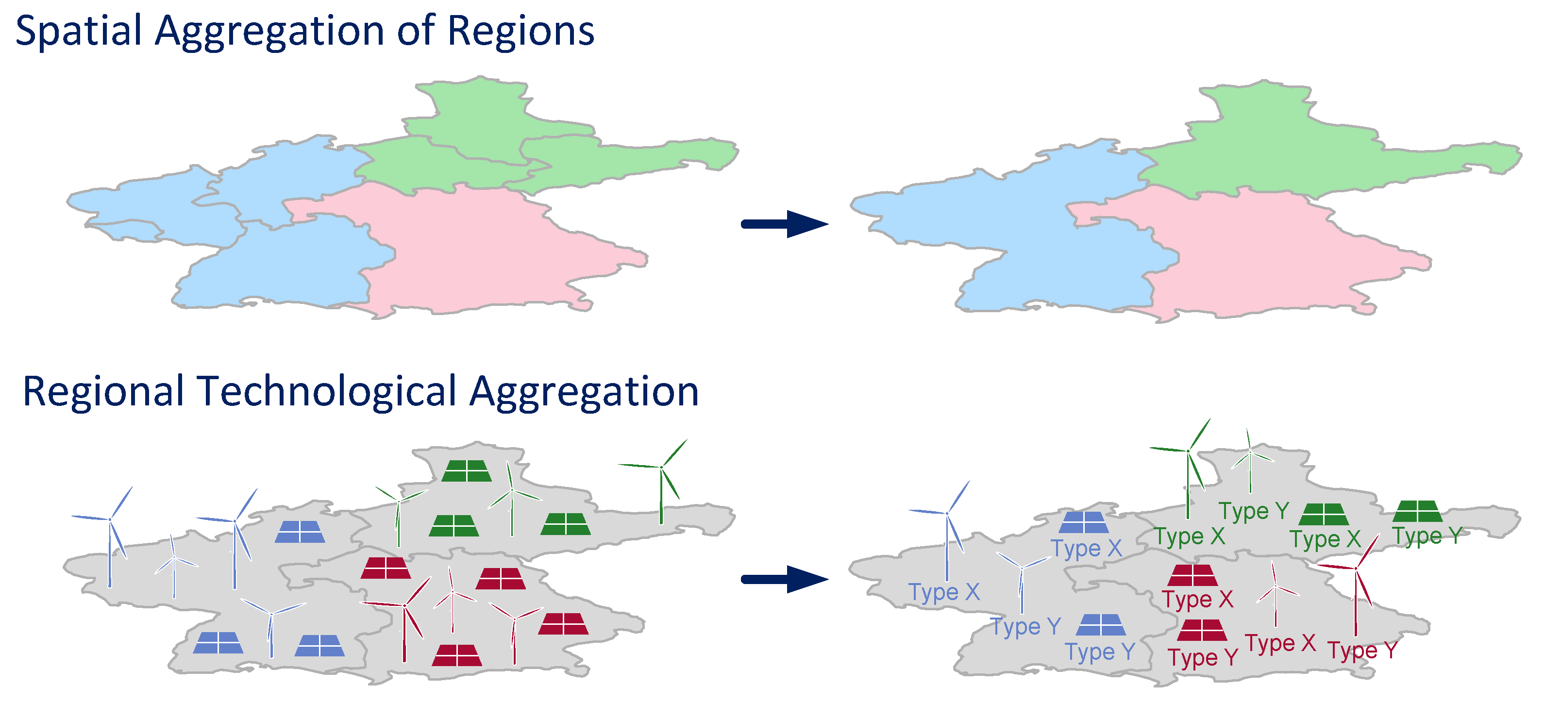
• First, the model regions are aggregated.
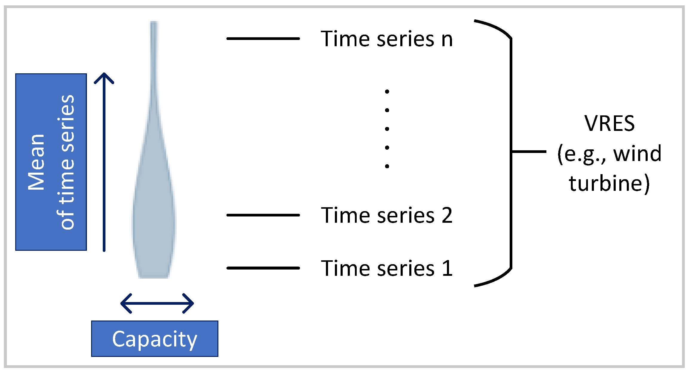
• Next, the CF time series of variable renewable energy source (VRES) (i.e., wind turbine and photovoltaic) are aggregated within each newly-defined region.

The remainder of this paper is structured as follows: Section 2 explores previous work on spatial and technological aggregation and identifies some research gaps and challenges associated with them. In Section 3, the developed aggregation methods that attempt to close these identified gaps and the abovementioned aggregation scheme are introduced. The experimental results are presented in Section 4. A summary and discussion can be found in Section 5. The main conclusions of the study are drawn in Section 6. Finally, some potential areas of future research are discussed in Section 7.

2. State of Research

2.1. Spatial Aggregation of Regions

According to Fischer [15], the aggregation of regions involves forming of homogeneous region sets from an initial set of regions. Each homogeneous set consists of spatially contiguous regions (i.e., neighboring regions) having a high degree of similarity with respect to an attribute or a set of attributes. In essence, aggregation of regions is a spatially constrained clustering problem. The four approaches to solving this problem are as follows: (i) sequentially applying a conventional clustering technique with no regard to geography and then only grouping similar regions identified if they are contiguous; (ii) adding x and y coordinates of each region’s centroid as its two additional attributes, thereby encouraging regions to group only with neighboring regions; (iii) explicitly including the spatial contiguity constraints in the clustering procedure; and (iv) employing graph-theory-based algorithms which reduce a connected graph into connected subgraphs, maximizing a similarity criterion within each of them [16].

In the context of energy systems analysis, spatial aggregation is commonly viewed as a network reduction problem. For instance, Hörsch and Brown [17] considered the European electricity transmission network and applied k-means clustering [18] to reduce this network. The aim here is to reduce the network while maintaining the major transmission corridors. The attributes considered for similarity definition are demand and generation capacities. In addition to these attributes, geographical locations are considered to ensure spatial contiguity.

According to Biener and Rosas [19], it is important to consider electrical grid characteristics during network reduction as it ensures accurate grid representation in the reduced ESOM. To that end, they introduced a network reduction method that takes electrical distances between nodes as the similarity defining attribute. A combination of density-based graph clustering [20] and agglomerative hierarchical clustering [21] methods were used to cluster the nodes. Using quality indicators such as the root-mean-square error, they compared their method with the one developed by Hörsch and Brown [17]. Most of the quality indicators chosen showed that their method outperformed that developed by Hörsch and Brown [17].

Cao et al. [4] assessed the German transmission grid. They considered the marginal costs of the total power supply as the similarity defining attribute and spectral clustering [22]—a graph-theory-based algorithm was used to cluster the nodes. The number of clusters was set to 20 and the ESOM was run for both the reduced case and the fully resolved one. In comparison to the fully resolved case, the reduced case showed a deviation of $7.4\%$ in the optimization results, but the computing time was drastically reduced to $4.3\%$.

In the HotMaps Horizon2020 project [23], the European NUTS3 regions [24] are aggregated based on various energy potentials (e.g., wind, solar, agricultural residues potentials, etc.), economic (e.g., electricity and gas prices) and sociodemographic (e.g., population and GDP) attributes. Additionally, geographic locations are considered. k-means clustering is used to cluster the regions and the NbClust tool [25] is employed to identify the optimal number of clusters. The results show that NUTS3 regions can be reduced to 17 clusters. It is noteworthy that although the geographic locations of the regions are considered during clustering, not all regions in the clusters are contiguous.

The e-Highway2050 project [26] considers various attributes to define similarity between regions, such as population, mean wind speed and solar irradiation, installed thermal and hydro capacity, and agricultural areas and natural grasslands. These attributes are weighted according to their significance. In addition, geographic locations are considered. The clustering method employed is from the Python module ClusterPy [27]. The algorithm is run for one country at a time to avoid grouping the regions of different countries. Here, the European NUTS3 regions are reduced to 96 regions.

In contrast to the aforementioned works, Siala and Mahfouz [14] began with high-resolution raster data. They introduced a spatial aggregation based on k-means++ [28] and max-p regions [16] algorithms. The aggregation of the data cells was based on wind potential, photovoltaic potential, or electricity demand at a given time. An ESOM was run for each of these cases and the results were compared to the case of national borders. They concluded that region definitions based on any one of these characteristics lead to better optimization results compared to national borders. The attributes considered during spatial aggregation in the aforementioned works are summarized in

Table 1. The attributes consideredduring spatial aggregation in the previous publications.

Publication	Attributes Considered
[17]	Demand and generation capacities
	Geographic locations of the regions
[19]	Electrical distances between regions
[4]	Marginal costs of the total power supply
[23]	Energy potentials (e.g., wind, solar, agricultural residues potentials, etc.)
	Economic (e.g., electricity and gas prices)
	Sociodemographic (e.g., population and GDP)
	Geographic locations of the regions
[26]	Population
	Mean wind speed and solar irradiation
	Installed thermal and hydro capacity
	Agricultural areas and natural grasslands, etc.
	Geographic locations of the regions
[14]	Wind potential or photovoltaic potential or electricity demand

.

2.2. Technological Aggregation

In the literature, it is common to simply aggregate each ESOM component data within each defined region [11,12,14]. For instance, demand and generation time series are averaged and their capacities are summed [5]. However, some works investigate the clustering of time series applied to energy systems.

The clustering of demand time series is performed in some studies [29,30,31]. With respect to generation time series, Joubert and Vermeulen [32] optimized wind farm locations using mean-variance portfolio optimization method. In a preprocessing step, wind farms were clustered using agglomerative hierarchical clustering. The optimization was then run for different numbers of clusters and the results were compared with those obtained in the case of optimization run with unclustered data to determine the optimal number of clusters. The authors concluded that even in the case of optimal number of clusters, there was a marginal deviation in the optimization results compared to the unclustered solution. However, they noted that clustering of the data had the benefit of reducing computation times.

Munshi and Yasser [33] clustered photovoltaic time series. They applied various clustering approaches, ranging from conventional techniques such as k-means and hierarchical clustering, to genetic algorithms [34] such as ant colony and bat clustering. The authors concluded that bat clustering exhibited the best performance but is computationally intensive.

In the context of ESOMs, Caglayan et al. [35] addressed the aggregation of VRES. Here, the time series of each VRES were grouped based on their respective levelized cost of electricity (LCOE) and the time series within each group were averaged. This procedure was then repeated for all defined regions. It was seen that considering more than one VRES time series, per region, leads to a lower TAC compared to one VRES time series, per region. Increasing the VRES resolution makes more available cost-competitive locations to choose from, thereby bringing the overall system costs down.

Radu et al. [36] introduced a two-stage procedure to identify and retain only the most relevant VRES locations and discard those that have little impact on the results of optimization. In the first stage, a simplified version of the ESOM was run with a full set of VRES locations, and the locations chosen during the optimization were deemed relevant. In the second stage, the full version of the ESOM was run with these VRES locations. The performance was evaluated by comparing the results with those obtained when a full version of the ESOM was run with a full set of VRES locations. The results showed that more than $90\%$ of the relevant VRES locations were correctly identified by the procedure, and the memory consumption and solver time were reduced by up to $41\%$ and $46\%$, respectively.

Frysztacki et al. [37] demonstrated the combined effect of spatial and VRES resolution on the results of the ESOM. The spatial aggregation approach here is similar to the one seen in Hörsch and Brown [17]. They began with a fine spatial resolution with VRES sites simply aggregated in each of the regions. They considered a scenario where spatial aggregation was performed, but the VRES resolution was maintained as is. They compared the results to a scenario where the spatial aggregation was performed and the VRES sites were simply aggregated within each newly-defined region. The results showed that system costs are underestimated at low spatial resolutions, as network bottlenecks are not revealed at lower resolutions. On the other hand, low VRES resolutions overestimate system costs due to the unavailability of cost-competitive locations. The authors concluded that both network and VRES resolution should be sufficiently high to accurately estimate the optimal system costs. The VRES resolution reduction approaches applied to ESOMs in the aforementioned works are summarized in

Table 2. The VRES resolutionreduction approaches applied to energy system optimization models (ESOMs) in the previous publications.

Publication	VRES Resolution Reduction Approach (within Each Region)
[5,11,12,14]	Simply aggregating all the generation sites
[35]	Clustering based on levelized cost of electricity (LCOE) of each generation site
[36]	Running a simplified version of the ESOM to identify relevant generation sites
[37]	Simply aggregating all the generation sites within subregion groups

.

2.3. Research Gaps and Challenges

An ESOM has several components and corresponding attributes. The attributes could be (i) one-dimensional regional (region) such as photovoltaic capacity; (ii) two-dimensional regional (region × time) such as photovoltaic time series; and (iii) two-dimensional connection (region × region) attributes such as electrical distance between regions. A detailed data structure is given in the next section.

The choice of attributes considered during spatial aggregation of an ESOM depends on the research question or the aim of the analysis. For instance, if the aim is to determine optimal VRES capacities based on their potentials and existing transmission grid capacities, the choice of attributes would be the VRES capacities and time series and the grid capacities. In this case, the spatial aggregation method should be able to consider attributes with varying aforementioned dimensions.

Previous works on the spatial aggregation of ESOM consider attributes that are either one-dimensional regional [4,14,17,23,26,37] or two-dimensional connection [19]. In this paper, a spatial aggregation method is introduced that can consider the ESOM components’ attributes with varying dimensions. The challenge here is to handle the heterogeneous dataset. Along with varying dimensions, the attributes can have different data types and ranges, making it difficult to calculate the similarity between regions based on them.

Further, considering geographic locations as additional attributes during region grouping, to ensure spatial contiguity in the resulting region groups, is seen to be common in previous works. This, however, does not always ensure spatial contiguity, as seen in Scaramuzzino et al. [23]. This is especially true if several attributes are considered during grouping and all attributes are weighted equally. Therefore, explicitly including the spatial contiguity constraints during region grouping is more appropriate. The challenge, though, is to deal with the computational complexity that is involved in imposing these constraints [38].

Table 3. Comparison of the spatial aggregation approach proposed in this paper with the previous works.

Publication	One-Dimensional Regional Attributes Considered?	Two-Dimensional Regional Attributes Considered?	Two-Dimensional Connection Attributes Considered?	Spatial Contiguity Ensured?
[17,37]	✓	✗	✗	✓
[19]	✗	✗	✓	✓
[4]	✓	✗	✗	✓
[23]	✓	✗	✗	✗
[26]	✓	✗	✗	✓
[14]	✓	✗	✗	✓
This paper	✓	✓	✓	✓

compares the spatial aggregation approach proposed in this paper to the aforementioned works.

In the context of ESOMs, the previous works on technological aggregation do not consider aggregating based on the VRES time series. In this paper, we consider very highly resolved VRES data. We cluster each VRES in each region based on the similarity of VRES time series, and thereby to obtain a representative set. The justification for such an approach is that the temporal fluctuations present in the time series of VRES play a crucial role in the design of an energy system. Therefore, technological aggregation should aim to preserve these.

Finally, the proposed two-step aggregation scheme is data-centric rather than ESOM-centric. Therefore, the scheme can be applied to any highly resolved ESOM where modelers face run time issues due to the complexity of the ESOM.

3. Methodology

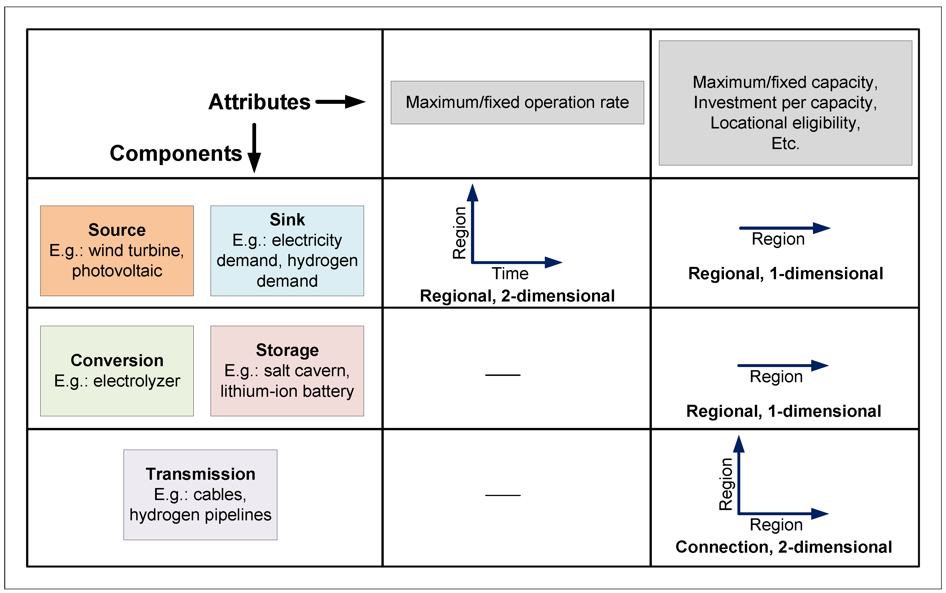
3.1. Energy System Optimization Model Details

For the analysis, an open-source optimization framework called the Framework for Integrated Energy System Assessment (FINE) [5] is employed. The mathematical formulation of FINE is given in Appendix A. Setting up an ESOM using FINE essentially involves adding various energy system components with their corresponding data. Figure 2 displays various component classes, their components, and data attributes corresponding to each. These attributes can be classified into two types:

• Regional attributes: These attributes are region-specific. They can be one-dimensional (region) or two-dimensional (region × time). Examples of one- and two-dimensional regional attributes are the maximum capacity and CF time series of a wind turbine, respectively.
• Connection attributes: These attributes characterize the connections between regions. They are always two-dimensional (region × region). An example of a connection attribute is the capacity of a DC cable between two regions.

Several attributes belonging to various system components, with varying dimensions, data types, and data ranges, make up a highly complex data structure. These data are stored as a netCDF file. Python’s xarray module [39] is used to read the saved netCDF files. The computations are then performed on the read-in xarray dataset.

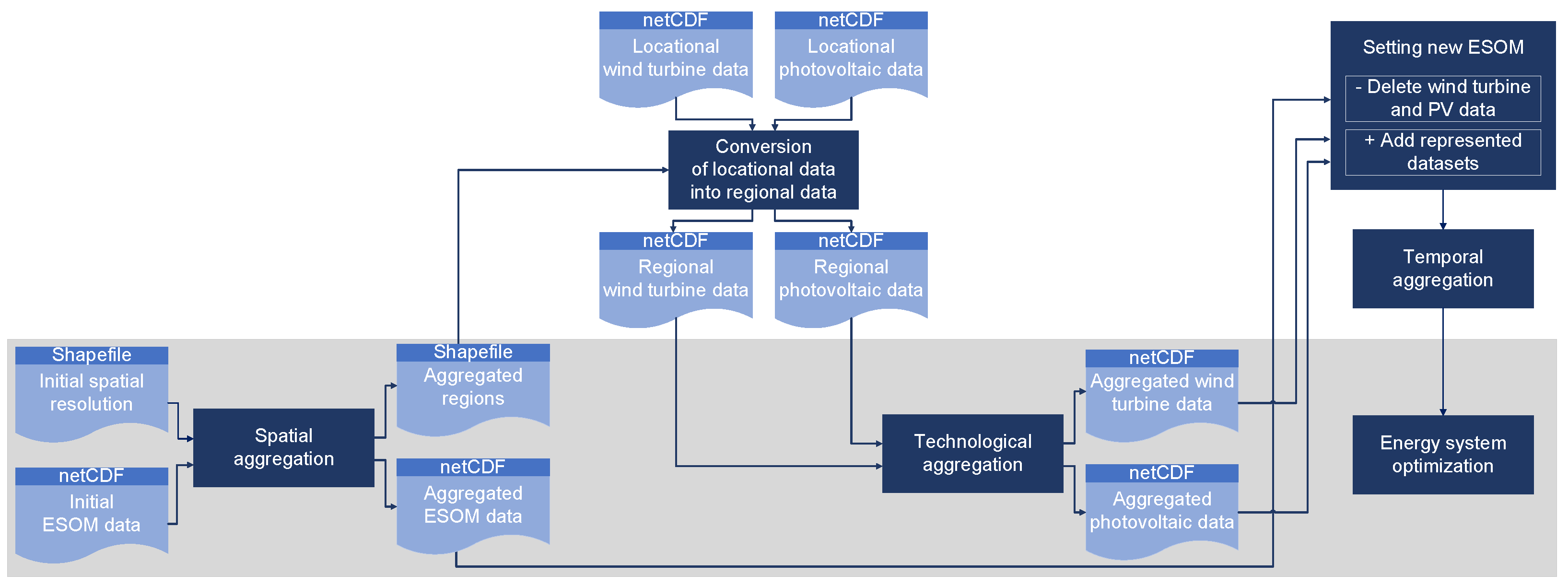
3.2. General Workflow

Figure 3 shows the general workflow adopted in this study. The highly resolved wind turbine and photovoltaic installations used in this study were obtained using the open-source tools Renewable Energy Simulation toolkit (RESKit) [40] and Geospatial Land Availability for Energy Systems (GLAES) [41]. These tools provide wind turbine and photovoltaic locations (x and y coordinates), capacities, and CF time series. To determine which of these locations belong to which regions, a geometric operation is performed where the locations are matched with the region geometries, which are present in a shapefile. Here, this operation is termed as conversion of locational data into regional data.

Initially, an ESOM is set up by adding various system components. In this ESOM, just one type of each component is present in each region. For instance, there is one photovoltaic in each region, which is an aggregation of all photovoltaics for that region. The spatial aggregation block takes as its input these ESOM data (in the form of a netCDF file) and a shapefile with the initial region geometries. It results in two outputs—a netCDF file and a shapefile with aggregated data and region geometries, respectively.

Next, conversion of locational data into regional data is performed with the aggregated region geometries. The output is fed to the technological aggregation block. Here, the aggregation is performed separately for wind turbines and photovoltaics.

Next, the wind turbines and photovoltaics present in the aggregated ESOM are replaced by the datasets resulting from technological aggregation. Further, to keep the computation time within reasonable limits, temporal aggregation is performed on the resulting dataset. Finally, optimization is performed on the aggregated ESOM.

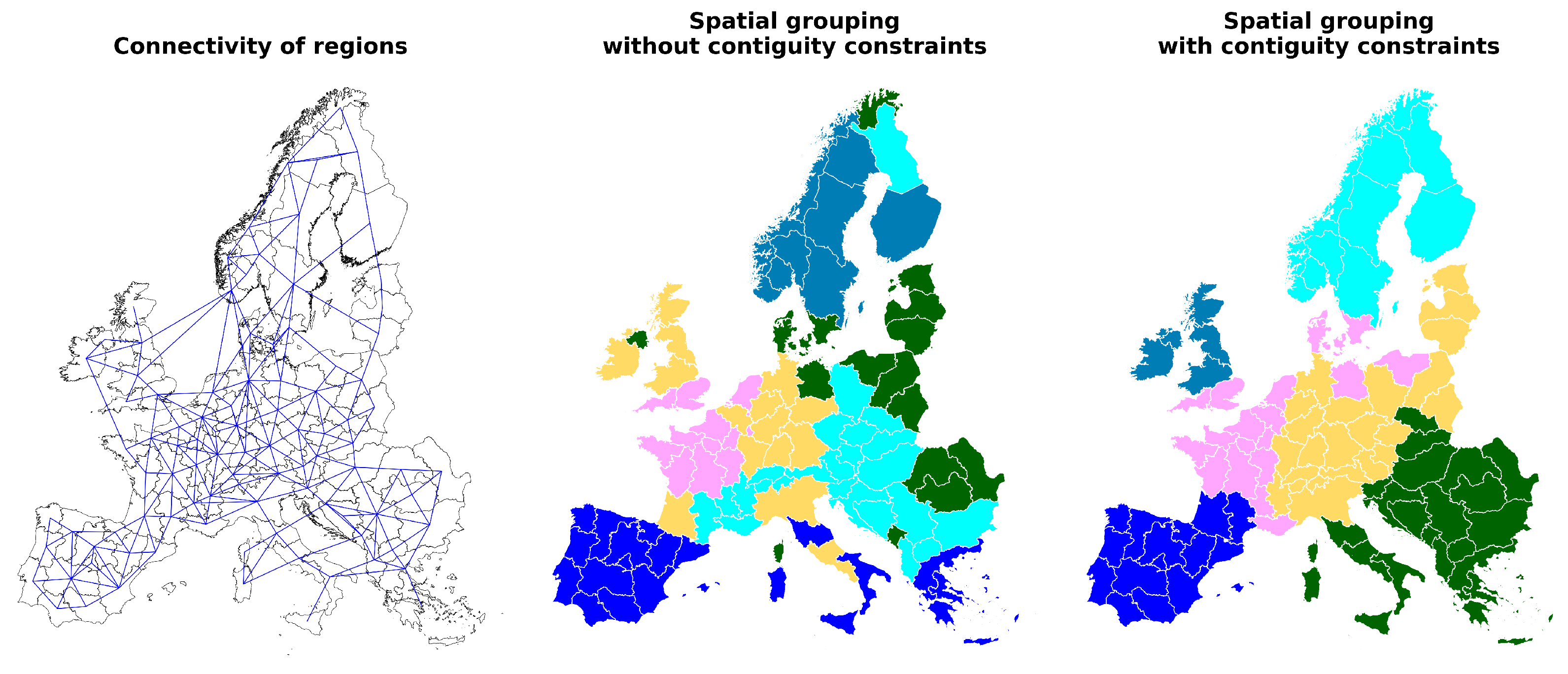
3.3. Spatial Aggregation

3.3.1. Algorithm

To aggregate the regions, the Hess model [42], also known as k-medoids clustering, is employed here. The aim is to partition a given region set V to form k groups.

If the number of regions in V is n and i and j are two arbitrary regions, then the Hess model uses the following $n^2$ binary variables:

$$\begin{array}{c}\hfill \left[H\right]x_{ij}=\left\{\begin{array}{cc}1,\hfill & \mathrm{if}i\mathrm{is}\mathrm{assigned}\mathrm{to}\mathrm{a}\mathrm{group}\mathrm{with}\mathrm{center}\mathrm{at}j\hfill \\ 0,\hfill & \mathrm{otherwise}.\hfill \end{array}\right.\end{array}$$

(1)

The Hess model is formulated in the following manner:

$$min\sum _{i\in V}\sum _{j\in V}D(i,j)x_{ij}$$

(2)

where $D(i,j)$ is the distance between the regions i and j.

It is subject to the following constraints:

$$\sum _{j\in V}{x}_{ij}=1\forall i\in V$$

(3)

$$\sum _{j\in V}{x}_{jj}=k$$

(4)

$$x_{ij}\le x_{jj}\forall i,j\in V$$

(5)

Constraints (3) ensure that each region is assigned to a group and only one group. Constraint 4 ensures that k groups are formed. Finally, Constraint (5) ensures that a region i is only assigned to region j if j is chosen to be a group’s center. In order to ensure spatial contiguity in the resulting region groups, contiguity constraints, first introduced by Oehrlein and Haunert [43] for spatial aggregation, are employed here. The constraint formulation is based on the concept of $(a,b)-separators$. An $(a,b)-separator$ can be defined as a subset of regions $C\subseteq V\backslash \{a,b\}$ that, if removed, would destroy all paths connecting regions a and b. Now, for regions a and b to belong to a group, at least one of the regions from C should also be present in this group. Otherwise, a and b would be disconnected. Mathematically, this condition is expressed as follows:

$$\sum _{c\in C}{x}_{cb}\ge x_{ab}\forall C\subseteq V\backslash \{a,b\}$$

(6)

With the aim of speeding up the calculations, the model is first solved without the contiguity constraints. The resulting region groups are scouted for disconnected region pairs and, subsequently, contiguity constraints for these region pairs are added and the model is solved again. This iterative process is stopped once all the regions in each group are connected (spatial aggregation code is published in the Python package https://github.com/FZJ-IEK3-VSA/tsam/blob/master/tsam/utils/k_medoids_contiguity.py (accessed on 4 October 2022)).

3.3.2. Distance Measure

As previously noted, the ESOM dataset has varying dimensions, data types, and ranges. No well-known distance function is capable of directly calculating the distance between regions in this case. Therefore, a custom distance is defined to calculate the distance between region pairs. This distance definition is based on the residual sum of squares and works on the values normalized across each data attribute. Mathematically, the distance between two regions a and b is defined as follows:

$$D(a,b)=D_{r\_1d}(a,b)+D_{r\_2d}(a,b)+D_{c\_2d}(a,b)$$

(7)

where

$D_{r\_1d}(a,b)$ is the cumulative distance of all one-dimensional regional attributes between the two regions, and is defined by:

$$D_{r\_1d}(a,b)=\sum _{i\in D_{r\_1d}}{\left(i\right(a)-i(b\left)\right)}^2$$

(8)

$D_{r\_2d}(a,b)$ is the cumulative distance of all two-dimensional regional attributes between the two regions, and is defined by:

$$D_{r\_2d}(a,b)=\sum _{i\in D_{r\_2d}}\sum _{t=1}^{t=T}{\left(i\right(a,t)-i(b,t\left)\right)}^2$$

(9)

Here, t = 1, 2,…,T are the time steps.

In addition, $D_{c\_2d}(a,b)$ is the cumulative distance of all two-dimensional connection attributes between the two regions, and is defined by:

$$D_{c\_2d}(a,b)=\sum _{i\in D_{c\_2d}}{(1-i(a,b\left)\right)}^2$$

(10)

Connection attributes indicate how strongly two regions are connected, and their normalized values lie in the range [0,1]. Therefore, these values are converted into a distance meaning by subtracting from 1, as shown in Equation (10).

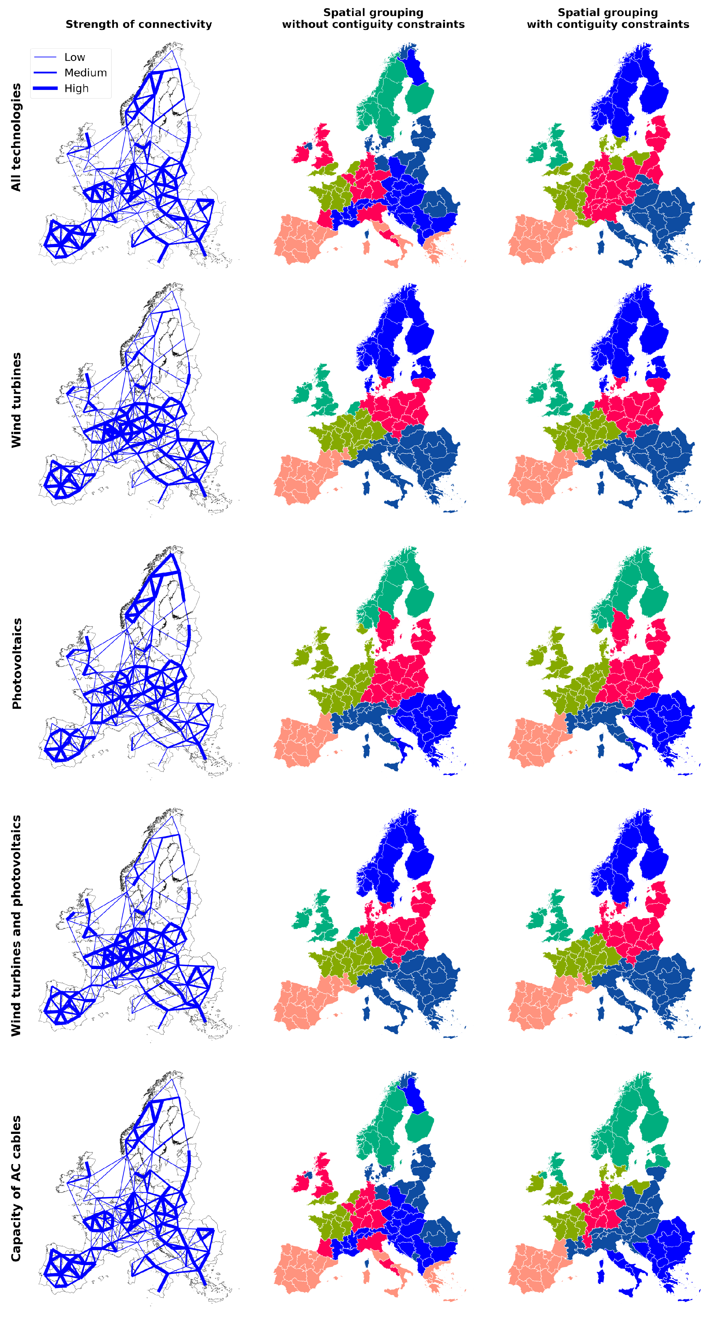
3.3.3. Connectivity Matrix

A connectivity matrix indicates which region pairs are connected and is employed in the algorithm described above to ensure spatial contiguity. In this matrix, the value corresponding to a region pair is 1 if they are spatially contiguous, otherwise 0. Two regions are deemed contiguous if:

• Their borders touch at least at one point;
• One of the regions is an island and the other its nearest mainland region;
• There is a transmission line or pipeline running between them.

3.3.4. Data Aggregation

Once the new region set is obtained, the data within each region group are aggregated. The aggregation method varies depending on the attribute. A list of all attributes and the aggregation method corresponding to each is presented in

Table 4. Aggregation method employed for each data attribute.

Attribute	Aggregation Method
Maximum time series	Weighted mean
	(weights: corresponding maximum capacity)
Fixed time series	Sum
Maximum capacity	Sum
Fixed capacity	Sum
Locational eligibility	Boolean OR
Investment per capacity	Mean
Investment if built	Boolean OR
Opex per operation	Mean
Opex per capacity	Mean
Opex if built	Boolean OR
Interest rate	Mean
Economic lifetime	Mean
Losses	Mean
Distances	Mean
Commodity cost	Mean
Commodity revenue	Mean
Opex per charge operation	Mean
Opex per discharge operation	Mean
Technical lifetime	Sum
Reactances	Sum

.

Note: The introduced spatial aggregation workflow allows the user to choose the attributes that should be used during region grouping, assign weights to each attribute, and override the default aggregation methods (shown in Table 4) to be used for each attribute after the regions are grouped (this spatial aggregation workflow is published in the Python package https://github.com/FZJ-IEK3-VSA/FINE/blob/master/FINE/aggregations/spatialAggregation/manager.py (accessed on 4 October 2022)).

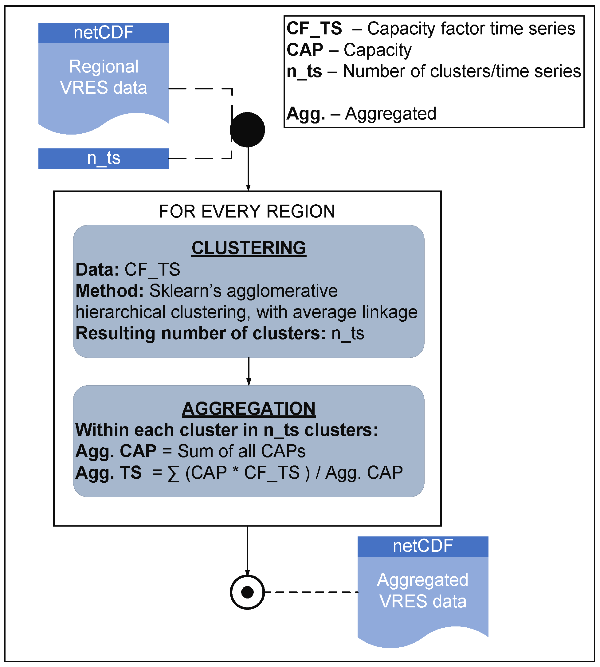
3.4. Technological Aggregation

The aggregation of VRES is based on their CF time series. In order to cluster the time series, different clustering techniques, such as k-means and agglomerative hierarchical clustering with different linkage criteria ([44]), were considered during the initial experimental phase. Among these techniques, agglomerative hierarchical clustering with average linkage showed better performance, but only marginally. Therefore, this method is considered here.

The agglomerative hierarchical clustering is a bottom-up approach in which each time series is initially treated as a cluster. At every iteration, the distance between cluster pairs is measured and the pair with the least distance is merged. This is repeated until the specified number of clusters is obtained.

Now, the linkage criteria help in measuring the distance between cluster pairs with more than one time series in them. The average linkage criterion measures the distance between two clusters based on the average of the distances between each member of one cluster and every member of the other cluster. Here, the basic distance measure is Euclidean distance.

This clustering technique is at the heart of the technological aggregation algorithm implemented. The flowchart of the algorithm is given in Figure 4. The regional VRES data (capacities and CF time series) of a particular VRES and the desired number ($n\_ts$) of time series per region are input. The algorithm works on one region at a time. First, the clustering technique is run. It clusters the time series to obtain $n\_ts$ clusters. Next, aggregation of the data is performed. Within each cluster, the aggregated capacity is the sum of all capacities belonging to that cluster. The aggregated time series is obtained by taking the weighted mean of all the time series belonging to the cluster, with the respective capacities being their weights (technological aggregation code is published in the Python package https://github.com/FZJ-IEK3-VSA/FINE/blob/master/FINE/aggregations/technologyAggregation/techAggregation.py (accessed on 4 October 2022)).

Note: As mentioned earlier, each region is assumed to be a lossless copper plate. The location of the VRES technologies within each region is irrelevant under this assumption. Since technological aggregation is performed within each region, the spatial contiguity problem does not arise here.

3.5. Experimental Design

3.5.1. Attributes Chosen for Spatial Aggregation

As mentioned before, the user can choose the attributes and their corresponding weights for spatial aggregation. For the analysis carried out in this paper, all the components’ attributes are used and all the attributes are weighted equally. The list of attributes is given in Table 4.

3.5.2. Spatial, Technological, and Temporal Scopes and Resolutions of ESOM

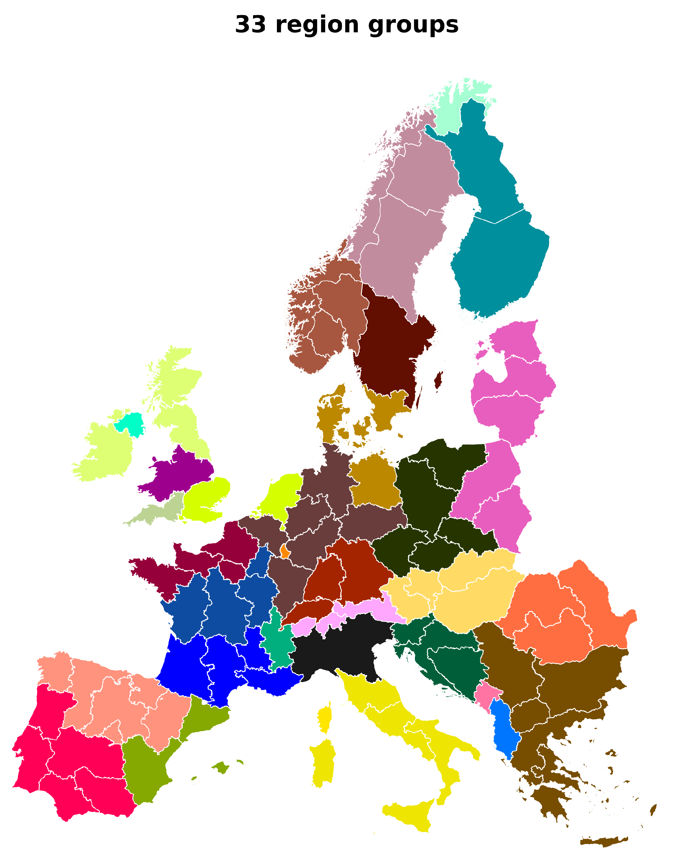
• Spatial scope and resolution: A European energy system scenario [35] is considered in this paper. The ESOM is set up for the same. As for the spatial resolution, the region definition suggested in the e-highway study is considered. In this study, the geographical area of Europe is divided into 96 regions.
• Technological scope and resolution: The wind turbines and photovoltaics are simulated for all of Europe. The result contains approximately 840,000 wind turbines and photovoltaics.
• Temporal scope and resolution: The data of one year are considered. They have an hourly temporal resolution, with 8760 time steps for one year. Prior to optimization, temporal aggregation is performed. The resolution is reduced to 40 typical days with eight segments within each typical day. For this purpose, the method developed by Hoffmann et al. [45] is employed.
  In order to accurately assess the impact of spatial and technological aggregations on the optimization results, the effects of temporal aggregation should be nullified across all experimental runs. Here, it is accomplished by performing temporal aggregation only for the highest spatial and technological resolution. The resulting temporal clusters are saved and in all the successive runs, the data are temporally aggregated to obtain the same clusters. This ensures that, in each case, the time series are reduced temporally to obtain the same set of typical days, with the same segments in each typical day.

3.5.3. Evaluation Method

In our analysis, the effects of the aggregations are evaluated based on two indicators—complexity and accuracy of the ESOM. The complexity indicator is the run time of optimization, and the accuracy indicator the optimization objective, i.e., the TAC.

Ideally, the results of the initial ESOM should be considered as a benchmark. However, considering 840,000 wind turbines and photovoltaics renders this ESOM instance computationally intractable.

The initial 96 regions consist of varying number of VRES time series. The lowest number of regional VRES time series is found to be 68. Therefore, initially the VRES time series in each region are aggregated to 68 VRES time series, such that this number is maintained in all the regions.

This combination of 96 regions and 68 VRES time series in each region forms the benchmark setting. The ESOM is optimized for this setting. Successively, various combinations of the number of aggregated regions and VRES time series per region are chosen and the procedure shown in Figure 3 is repeated. In each case, the TAC and run time are recorded and compared.

4. Results

4.1. Spatial Aggregation

For the purpose of comparison, the initial 96 regions are aggregated to obtain six region groups without and with the contiguity constrains. The results are shown in Figure 5 along with the connectivity of the regions, as per the obtained connectivity matrix.

When aggregation is performed without the contiguity constraints, the resulting region groups are not fully connected. For instance, the northernmost region in Norway is only connected to its immediate neighbors in Norway and Finland; however, it is grouped with some southern regions. A similar observation can be made with regard to other region groups too.

The plot on the right in Figure 5 indicates that aggregating the regions with contiguity constraints ensures the formation of region groups that are fully connected. Here, all the regions are compact except the one shown in pink, which has some fragmented parts. Nonetheless, the original regions present in this group are connected, and therefore the contiguity constraints are not violated here.

It is noteworthy that the time taken to aggregate the regions without and with contiguity constraints is 0.15 and 1.33 min, respectively. This indicates that imposing contiguity constraints, although necessary, is computationally taxing.

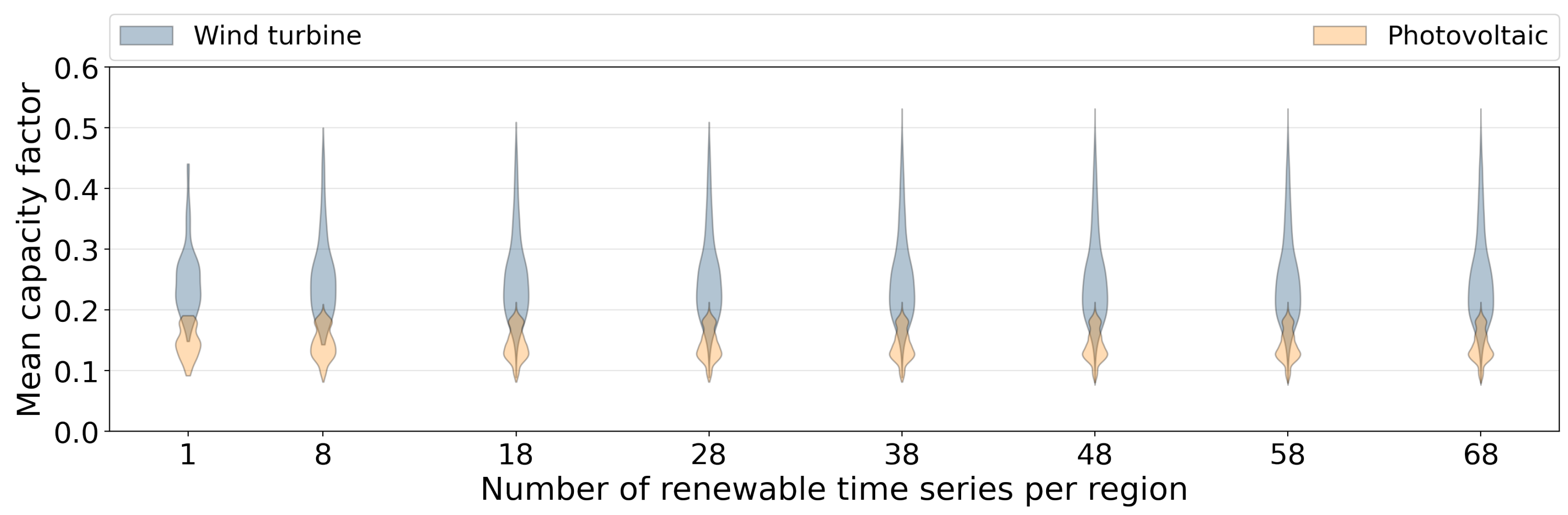
4.2. Technological Aggregation

Here, the results of technological aggregation are analyzed using the capacity distribution curves. An example capacity distribution curve is shown in Figure 6. The y-axis indicates the mean of each VRES time series. The width of the curve, corresponding to each y-value, shows the capacity corresponding to the VRES time series.

For the 96 regions, the technological aggregation algorithm is run to obtain different number of VRES time series per region. The capacity distribution curves in each case are depicted in Figure 7. In both the distributions, at lower numbers of VRES time series the extreme values are not captured well. As the number of VRES time series is increased, the extreme values appear. At 38 VRES time series, all of the extreme values seem to be captured, as a further increase in the number of VRES time series does not change the distribution of both photovoltaic and wind turbine data.

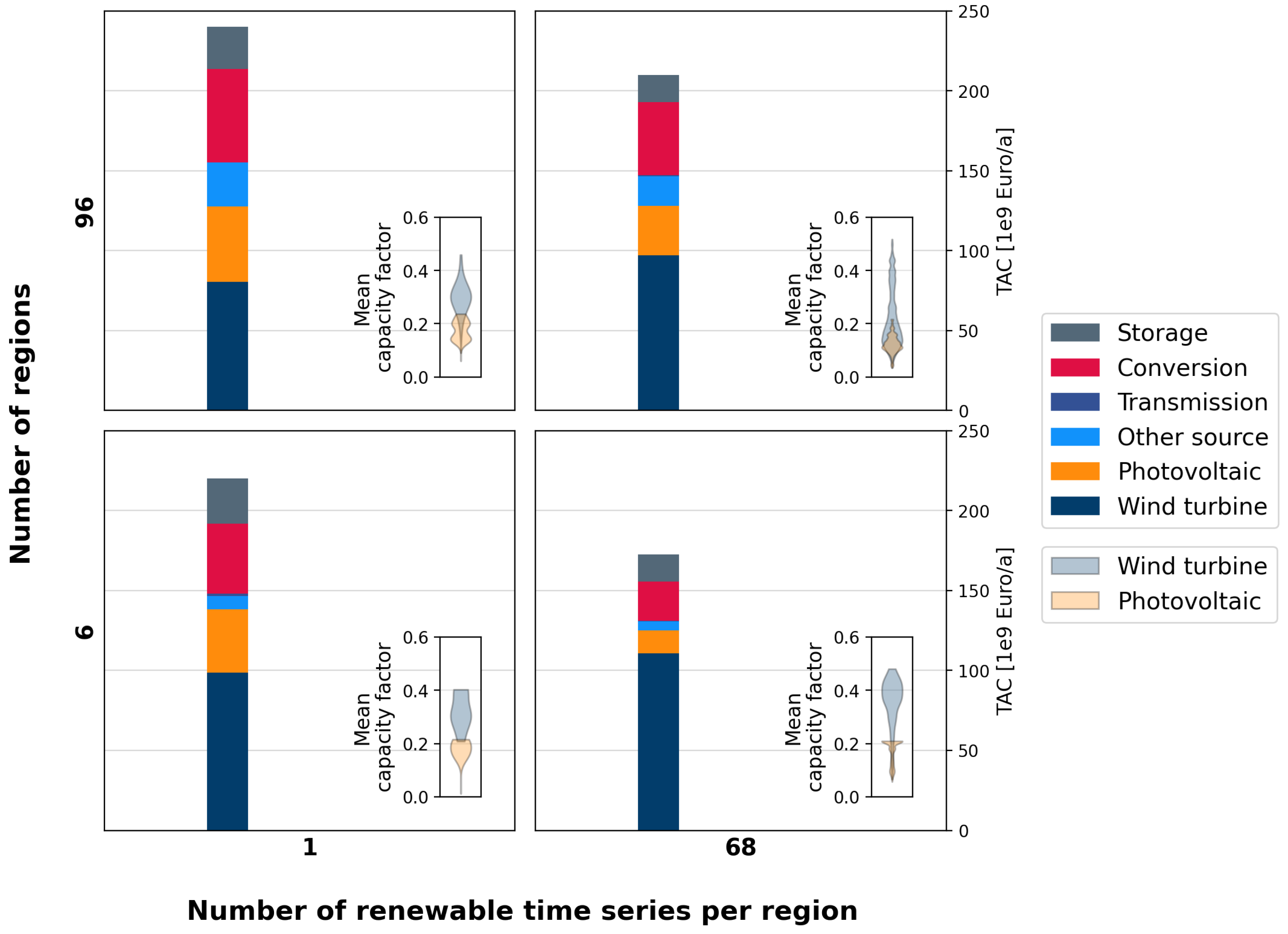
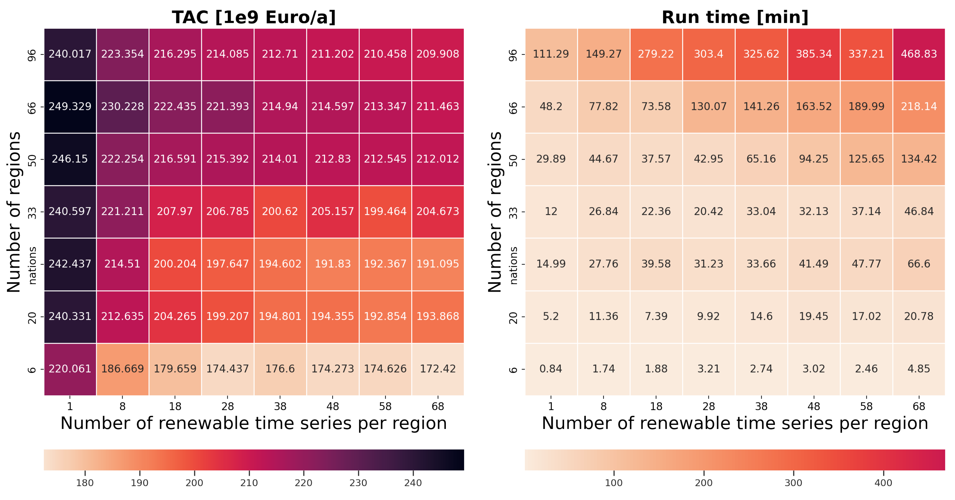
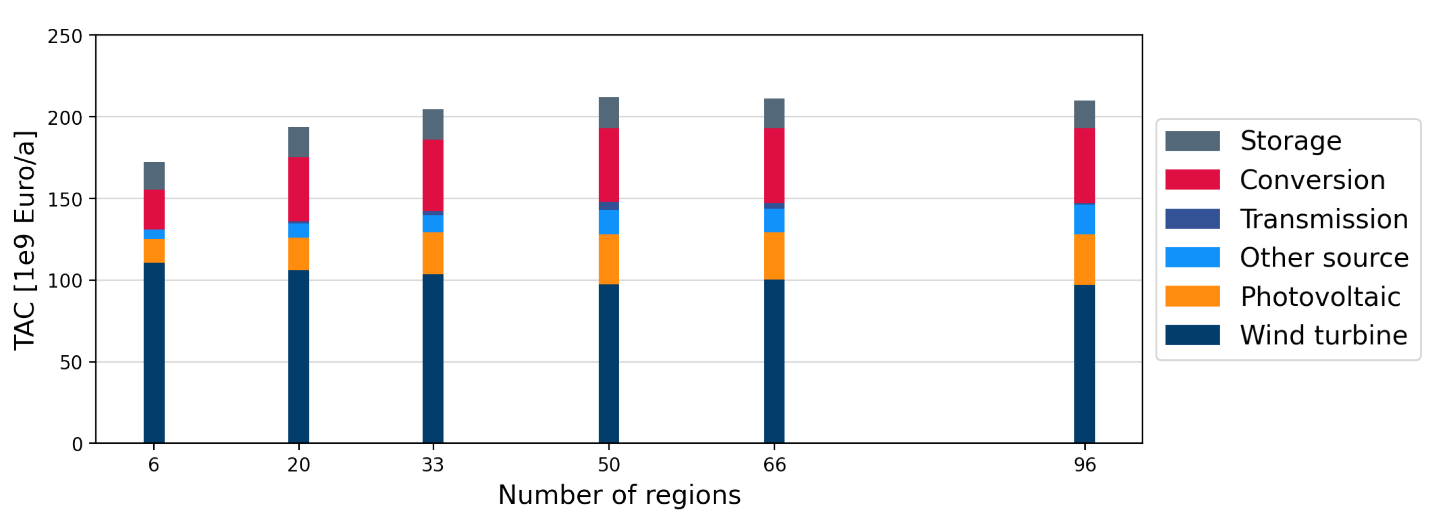
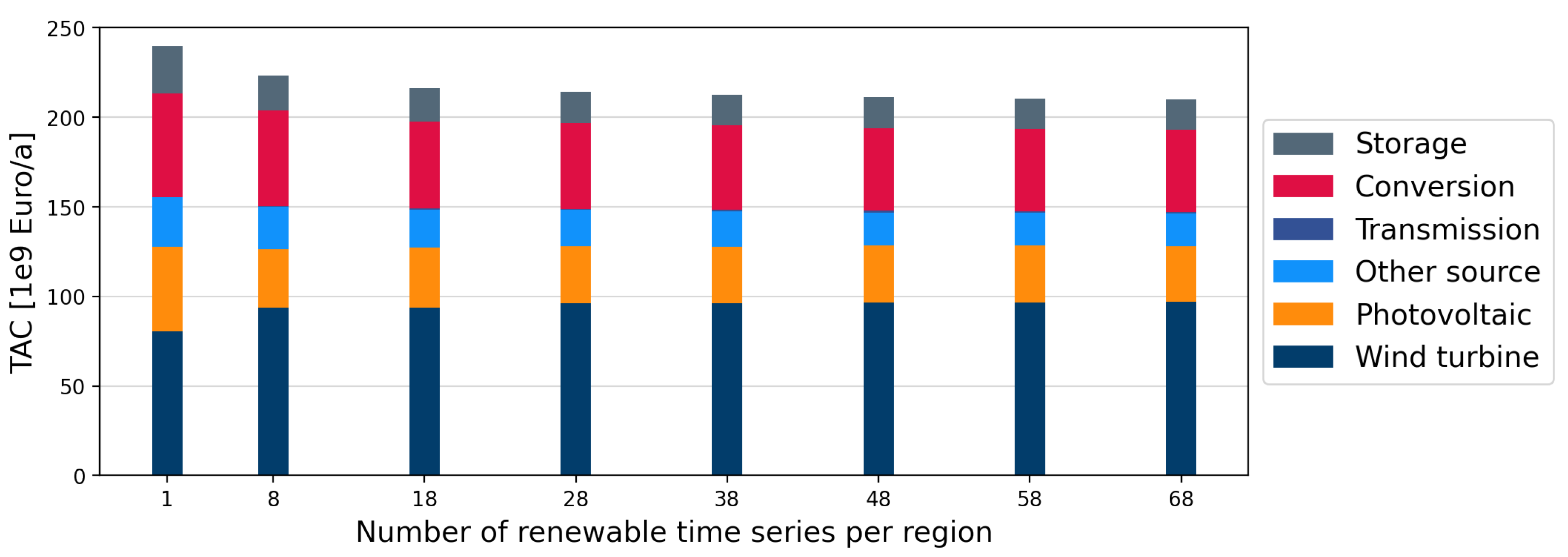
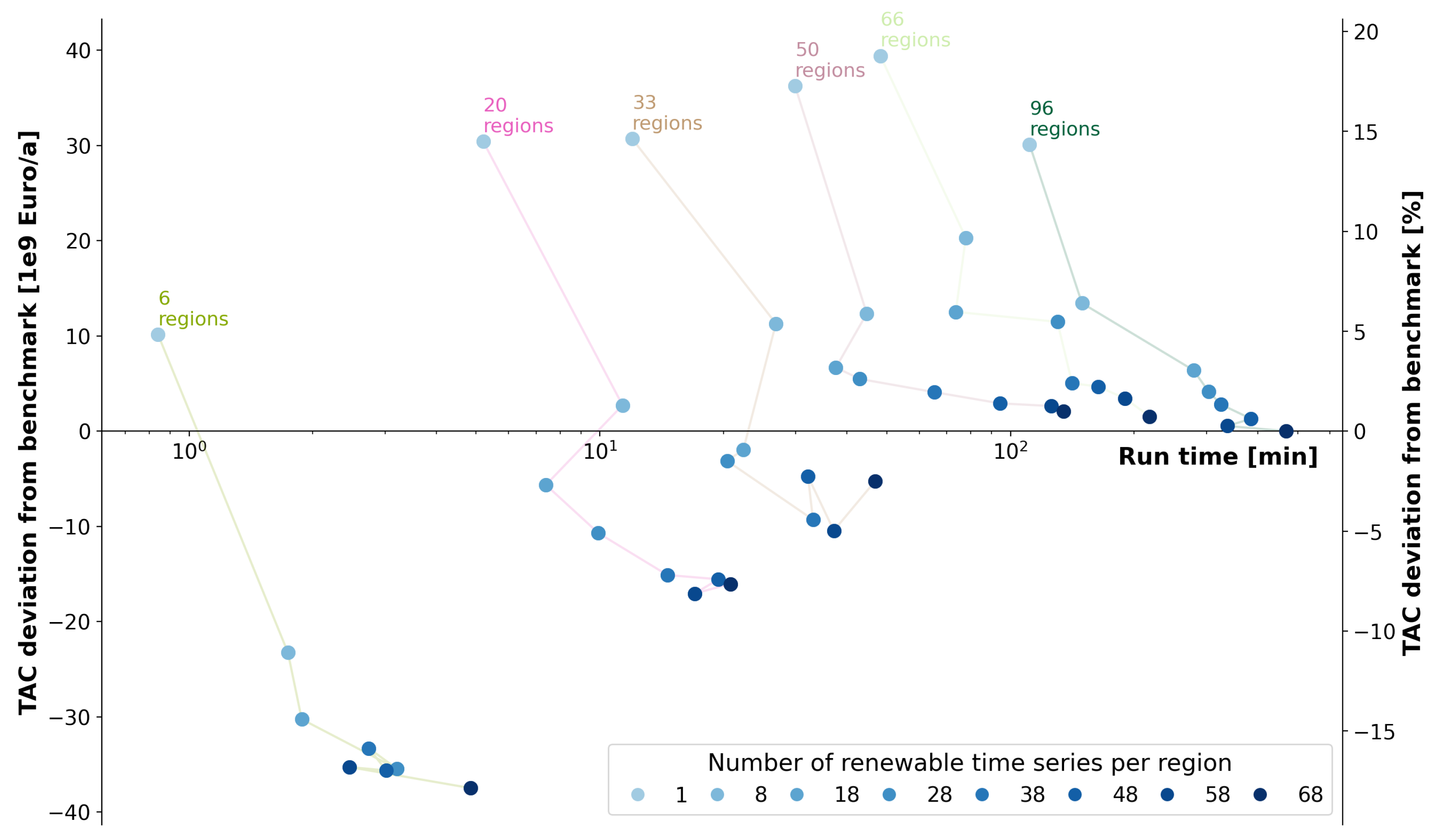
4.3. Impact of Spatial and Technological Aggregation on Optimization Results

The lowest and highest numbers of regions considered in this study are 6 and 96, respectively. The lowest and highest numbers of VRES time series per region considered are 1 and 68, respectively. Initially, the optimization results obtained for these extreme combinations are analyzed. Figure 8 shows the optimization results for these parameter combinations. For each parameter setting, a bar plot on the left shows TAC for different technologies, and on the right, distribution of installed VRES capacities (i.e., the distribution of optimal capacity and operational time series chosen during optimization).

The top-right cell in this figure shows the benchmark results, i.e., the results for 96 regions with 68 VRES time series per region. With this setting, the overall TAC is approximately EUR 210 billion/annum. The wind turbine’s capacity distribution curve starts with a needle-like shape around 0.52 mean CF and slowly widens for lower mean CFs and narrows again at a mean CF around 0.1. The photovoltaic’s capacity distribution curve also has a similar shape. It starts at around 0.2 mean CF and slowly widens and narrows again at a mean CF around 0.1.

The top-left cell shows the optimization results when the number of regions is kept the same but the number of VRES time series is reduced to one per region. It can be observed that reducing the number of VRES time series, while keeping the number of regions constant, leads to an increase in the TAC. The capacity distributions of VRES help explain this behavior. It is seen in Figure 7 that the extreme values are not well captured when one VRES time series per region is considered. Due to the fact that wind turbines with high mean CFs are not available to choose from, most wind turbines that are installed have mean CFs around 0.3. In comparison to the benchmark, fewer wind turbines are installed, bringing the TAC of wind turbines down. As an alternative, more photovoltaics and other source technologies are installed, thereby increasing their TACs. Increases in the installation of these technologies requires an increase in the installation of conversion and storage technologies. Therefore, the TAC of these technologies also increases.

In the bottom-right cell, the optimization results obtained when the number of regions is reduced to six and the number of VRES time series per region is 68 are shown. It can be observed that reducing the number of regions leads to a decrease in the TAC. As each region is considered a single node under the copper plate assumption, the size of these regions does not play a role during optimization. In other words, it does not matter if these regions are spread across Europe or just a single country. The spatial details within these regions is also limited, as each component is aggregated within them. These factors give it the effect of the energy system being small with a network of six regions, leading to an underestimation of the overall TAC.

In this setting, each of the six regions now has 68 VRES time series, as opposed to the benchmark setting, where each of the 96 regions have 68 VRES time series. In comparison to the benchmark, the wind turbine’s capacity distribution shows that the peaks are not captured well in this setting, thereby installing more wind turbines with mean CFs around 0.4. When good locations for wind turbine installation are found in each region, owing to the size of these and the copper plate assumption, there is less of a need for alternative sources. Therefore, in comparison to the benchmark, more wind turbines and fewer photovoltaics and other sources are installed here. Owing to the decrease in the installation of these technologies, a decrease in the installation of conversion and storage technologies is observed.

Finally, the bottom-left cell displays the effect of reducing both the number of regions and the number of VRES time series per region. In comparison to the benchmark, both the overestimation of the TAC due to the decrease in the number of VRES time series and the underestimation due to the decrease in the number of regions are apparent here. The overall TAC is approximately EUR 220 billion/annum. It comes close to the benchmark value. However, individual TACs and associated capacity distributions differ.

The wind turbine’s capacity distribution shows that only those with mean CFs between 0.2 and 0.4 are installed in this setting. Due to the unavailability of better locations for wind turbines, more photovoltaics with mean CFs around 0.2 are installed. Other sources are installed less when compared to the benchmark, leading to a decrease in the installation of conversion technologies. On the other hand, increases in photovoltaic installation have led to the increased installation of storage technologies.

Figure 9 shows the TAC obtained and the associated run time for each parameter setting considered in this study. The general observation made earlier—that decreasing the number of regions leads to a decrease in the TAC, and reducing the number of VRES time series per region increases it—holds true overall. The run time is high for the benchmark setting and reduces in both the directions.

It is noteworthy that in both the TAC and run time matrices, some exceptions to the general observations are visible. For instance, in the case of 33 aggregated regions, reducing the VRES time series from 58 to 48 leads to an increase in the TAC, but further reducing it to 38 VRES time series decreases the TAC. Furthermore, the run time for 96 regions and 58 VRES time series is 337.21 min. However, when the model is optimized for 96 regions and 48 VRES time series, the run time increases to 385.24 min. The reason for such exceptions could be that it is more challenging to find a global minimum in the case of certain region groups and the set of representative VRES time series within these.

In addition to the different number of aggregated regions, the results for 33 national regions can also be seen in Figure 9. Comparing the TACs obtained for 33 nations and 33 aggregated regions with the benchmark values, it can be observed that the TACs obtained for 33 nations deviate further from the benchmark. This shows that considering administrative boarders while designing an optimal energy system does not yield the best results.

Figure 10 shows the TAC for different technologies when the number of regions is varied while considering 68 VRES time series within each region in each case. It can be observed that as the number of regions is increased, the overall TAC shows a drastic increase at first and reaches a point of stabilization, whereas a further increase in the number of regions seems to have no significant effect on the TACs. Here, the optimal number of regions can be determined using the elbow criterion, i.e., the number of regions where a further increase would not significantly change the TACs. Similarly, in Figure 11 where the number of VRES time series is varied for 96 regions, the optimal number of VRES time series per region would be the number of VRES time series where the TACs stabilize.

In order to determine the optimal combination of the number of aggregated regions and VRES time series within each of them, it is necessary to apply the elbow criterion in both the directions of increase. In Figure 12, the run time (represented on a logarithmic scale on the x-axis) and TAC deviation from the benchmark (represented on the y-axis in EUR billion/annum on the left and in % on the right) for each parameter setting can be seen. Each dot represents a particular parameter setting. The darker the shade of blue, the greater the number of VRES time series considered, and the lines connecting the dots represent a particular number of regions.

From the figure, it can be observed that for each region set, as the number of VRES time series is increased, the deviation is drastically reduced at first and seems to stabilize after a certain number of VRES time series. On the other hand, keeping the number of VRES time series per region constant, if the number of regions is increased, the deviation stabilizes, approaching 0 in each case. Another noteworthy observation is that although the run time increases when the number of regions is increased or the number of VRES time series per region is increased, this increase is relatively more drastic in the case of increase in the number of regions.

With the aim of determining an optimal parameter combination, a matrix containing TAC for each parameter combination is traversed. For each combination, the TACs in both the directions of increase are compared with the benchmark value. If the percentage error between the benchmark TAC and each of the candidate TACs is below an acceptable error threshold, then the parameter combination is deemed to be optimal and the search is terminated. Here, an error threshold of $\pm 5\%$ is assumed. In terms of absolute value, the error threshold is approximately EUR $\pm 10$ billion/annum. Using this method, 33 aggregated regions and 38 VRES types in each region are deemed to be optimal. With this setting, the TAC obtained and the run time are EUR 200.62 billion/annum and 33.04 min, respectively. In comparison to the benchmark, the TAC is underestimated by EUR 9.29 billion/annum and the run time is reduced by 435.79 min in this case. The optimal 33 region groups formed are shown in Figure 13.

5. Summary and Discussion

For different combinations of numbers of regions and VRES within each, the objective TAC resulting from model optimization and the run time were compared to the benchmark setting of 96 regions and 68 VRES types in each region.

Furthermore, as it is common to consider administrative regions such as national borders when designing an optimal energy system, the study also considered 33 national regions. Moreover, it is standard practice to aggregate all system components, including VRES, within each model region to obtain just one representative type. This setting was also considered in this study.

The TACs obtained in the case of 33 national regions and 33 aggregated ones were compared to the benchmark. It was observed that the TAC obtained in the case of 33 national regions deviated further from the benchmark, compared to the case of the 33 aggregated regions. As each model region is assumed to be a copper plate and the system components are aggregated in each, it is important to pay attention to the region definitions. The defined regions should have similar component characteristics such that an aggregation of these components would not lead to a loss of information, which in turn leads to high TAC deviations.

To that end, considering a very low number of aggregated regions (for, e.g., six regions in Europe) would also result in high TAC deviations, even though the VRES resolution is maintained sufficiently high in each of these regions. In such cases, there is an oversimplification of the region network. In other words, the geographical gaps between generation and demand sites are largely ignored. This leads to an underestimation of the TAC.

Even when 96 regions were considered, considering one representative VRES per region led to a large deviation in the objective TAC. Here, the temporal fluctuations present in the original set of VRES time series are not well captured. Furthermore, the TAC is overestimated because cost-competitive locations are not identified at such a low VRES resolution. Therefore, irrespective of the spatial resolution of a model, the VRES resolution should be maintained sufficiently high in each region.

The elbow criterion shows that beyond a particular number of regions, a further increase in this number does not lead to a significant gain in accuracy, and yet the run time increases. Therefore, it is only logical that beyond a certain spatial resolution, a further gain in the accuracy can only be achieved by increasing the technological details, such as the number of VRES time series, within regions.

Regarding the optimal combination of spatial and technological resolution, it is seen that at 33 aggregated regions and 38 representative VRES in each, the system cost is underestimated by $4.42\%$ and the run time reduced by $92.95\%$, compared to the benchmark. A further increase in the spatial resolution does not significantly improve the results, thereby making this setting optimal for a European energy scenario considered in this study.

6. Conclusions

In this study, new spatial and technological aggregation methods were introduced. The spatial aggregation method can consider all or a subset of energy system model parameters to find and group homogeneous regions. The modeler can also assign weights to these attributes. Considering several attributes during region grouping runs the risk of resulting in spatially fragmented regions. However, our method allows only spatially contiguous regions to be grouped, irrespective of the number of attributes considered during region grouping. Such a method allows the modeler to base the spatial aggregation on a certain set of attributes, depending on the aim of the analysis.

Regarding the introduced technological aggregation method, a time series aggregation technique was employed to cluster variable renewable technologies, such as wind turbines and photovoltaics, based on the similarity of their time series, to obtain a representative set. Such a method reduces computational complexity while capturing the temporal fluctuations that are crucial for an accurate energy system design. Furthermore, the study introduced a scheme that facilitates simultaneous spatial and technological aggregation of energy system models as a complexity-reduction technique. This scheme is model-agnostic, i.e., it can be easily applied to any energy system model.

The introduced scheme was applied to a highly resolved European energy scenario. Here, the spatial aggregation was performed based on all the model parameters. Our results show that both spatial and technological resolutions should be maintained sufficiently high in order to obtain accurate optimization results. However, beyond a certain spatial resolution, a further increase does not significantly improve the accuracy. Therefore, we recommend that the modelers should choose an appropriate spatial resolution and further increase the technological details within the regions.

Although the introduced scheme is model-agnostic, the identification of the optimal combination of spatial and technological resolution is model-dependent. An optimal combination depends on the spatial and temporal scope of the model. Furthermore, when aggregated system states are linked—either in space or time—by transmission or storage, or have nonlinear relations, the inherent system behavior cannot be easily predicted. In consequence, the aggregation scheme needs to be applied to the target model and run some tests. This, however, does not necessarily require the model to be run with full resolution to determine the target accuracy. One could begin with a low resolution and increase it further. If the results do not vary significantly, it is an indication that a saturation has been reached in terms of accuracy.

7. Outlook

Some future areas of research:

• In our analysis, we consider all the model parameters for spatial aggregation. In Appendix B, we show how the region groups differ when different sets of attributes are chosen for spatial aggregation. However, it would be interesting to perform a detailed sensitivity analysis.
• Our focus in this paper was to sufficiently represent variable renewable energy sources in each region. It would also be interesting to increase the spatial details of other components, such as storage technologies, and investigate the extent of their influence on energy system design.
• Certain combinations of spatial and technological aggregations would also be worth investigating. For example, spatial aggregation based on electricity grid, and maintaining the spatial resolution of both source and storage technologies sufficiently high in each region.
• We performed a spatial and technological aggregation and then a temporal aggregation in our experiments reported herein. It would be worth investigating the effect of a switch in this order and to determine an optimal combination of spatial, technological, and temporal resolutions.

8. Code Availability

The workflow introduced in this paper is published in the Python package https://github.com/FZJ-IEK3-VSA/FINE/tree/master/FINE/aggregations (accessed on 4 October 2022). These methodologies can be easily applied and extended. For a demo of the workflow, please refer to the https://github.com/FZJ-IEK3-VSA/FINE/tree/master/examples/Spatial_and_technology_aggregation (accessed on 4 October 2022).

References

1. Agreement, P. Paris agreement. In Proceedings of the Report of the Conference of the Parties to the United Nations Framework Convention on Climate Change (21st Session, 2015: Paris), Retrived December, HeinOnline, Paris, France, 30 November–15 December 2015; Volume 4, p. 2017. [Google Scholar]
2. Samsatli, S.; Samsatli, N.J. A general spatio-temporal model of energy systems with a detailed account of transport and storage. Comput. Chem. Eng. 2015, 80, 155–176. [Google Scholar] [CrossRef]
3. DeCarolis, J.; Daly, H.; Dodds, P.; Keppo, I.; Li, F.; McDowall, W.; Pye, S.; Strachan, N.; Trutnevyte, E.; Usher, W.; et al. Formalizing best practice for energy system optimization modelling. Appl. Energy 2017, 194, 184–198. [Google Scholar] [CrossRef] [Green Version]
4. Cao, K.K.; Metzdorf, J.; Birbalta, S. Incorporating power transmission bottlenecks into aggregated energy system models. Sustainability 2018, 10, 1916. [Google Scholar] [CrossRef] [Green Version]
5. Welder, L.; Ryberg, D.S.; Kotzur, L.; Grube, T.; Robinius, M.; Stolten, D. Spatio-temporal optimization of a future energy system for power-to-hydrogen applications in Germany. Energy 2018, 158, 1130–1149. [Google Scholar] [CrossRef]
6. Samsatli, S.; Samsatli, N.J. A multi-objective MILP model for the design and operation of future integrated multi-vector energy networks capturing detailed spatio-temporal dependencies. Appl. Energy 2018, 220, 893–920. [Google Scholar] [CrossRef]
7. Pfenninger, S.; Hawkes, A.; Keirstead, J. Energy systems modeling for twenty-first century energy challenges. Renew. Sustain. Energy Rev. 2014, 33, 74–86. [Google Scholar] [CrossRef]
8. Ridha, E.; Nolting, L.; Praktiknjo, A. Complexity profiles: A large-scale review of energy system models in terms of complexity. Energy Strategy Rev. 2020, 30, 100515. [Google Scholar] [CrossRef]
9. Priesmann, J.; Nolting, L.; Praktiknjo, A. Are complex energy system models more accurate? An intra-model comparison of power system optimization models. Appl. Energy 2019, 255, 113783. [Google Scholar] [CrossRef]
10. Frew, B.A.; Jacobson, M.Z. Temporal and spatial tradeoffs in power system modeling with assumptions about storage: An application of the POWER model. Energy 2016, 117, 198–213. [Google Scholar] [CrossRef] [Green Version]
11. Kotzur, L.; Nolting, L.; Hoffmann, M.; Groß, T.; Smolenko, A.; Priesmann, J.; Büsing, H.; Beer, R.; Kullmann, F.; Singh, B.; et al. A modeler’s guide to handle complexity in energy system optimization. arXiv 2020, arXiv:2009.07216. [Google Scholar] [CrossRef]
12. Cao, K.K.; von Krbek, K.; Wetzel, M.; Cebulla, F.; Schreck, S. Classification and evaluation of concepts for improving the performance of applied energy system optimization models. Energies 2019, 12, 4656. [Google Scholar] [CrossRef] [Green Version]
13. Grubesic, T.H.; Wei, R.; Murray, A.T. Spatial clustering overview and comparison: Accuracy, sensitivity, and computational expense. Ann. Assoc. Am. Geogr. 2014, 104, 1134–1156. [Google Scholar] [CrossRef]
14. Siala, K.; Mahfouz, M.Y. Impact of the choice of regions on energy system models. Energy Strategy Rev. 2019, 25, 75–85. [Google Scholar] [CrossRef]
15. Fischer, M.M. Regional taxonomy: A comparison of some hierarchic and non-hierarchic strategies. Reg. Sci. Urban Econ. 1980, 10, 503–537. [Google Scholar] [CrossRef]
16. Duque, J.C.; Anselin, L.; Rey, S.J. The max-p-regions problem. J. Reg. Sci. 2012, 52, 397–419. [Google Scholar] [CrossRef]
17. Hörsch, J.; Brown, T. The role of spatial scale in joint optimisations of generation and transmission for European highly renewable scenarios. In Proceedings of the 2017 14th International Conference on the European Energy Market (EEM), IEEE, Dresden, Germany, 6–9 June 2017; pp. 1–7. [Google Scholar]
18. Lloyd, S. Least squares quantization in PCM. IEEE Trans. Inf. Theory 1982, 28, 129–137. [Google Scholar] [CrossRef] [Green Version]
19. Biener, W.; Rosas, K.R.G. Grid reduction for energy system analysis. Electr. Power Syst. Res. 2020, 185, 106349. [Google Scholar] [CrossRef]
20. Zhou, Y.; Cheng, H.; Yu, J.X. Graph clustering based on structural/attribute similarities. Proc. Vldb Endow. 2009, 2, 718–729. [Google Scholar] [CrossRef] [Green Version]
21. Ward, J.H., Jr. Hierarchical grouping to optimize an objective function. J. Am. Stat. Assoc. 1963, 58, 236–244. [Google Scholar] [CrossRef]
22. Fiedler, M. Algebraic connectivity of graphs. Czechoslov. Math. J. 1973, 23, 298–305. [Google Scholar] [CrossRef]
23. Scaramuzzino, C.; Garegnani, G.; Zambelli, P. Integrated approach for the identification of spatial patterns related to renewable energy potential in European territories. Renew. Sustain. Energy Rev. 2019, 101, 1–13. [Google Scholar] [CrossRef] [Green Version]
24. Eurostat, N. Nomenclature of Territorial Units for Statistics; Eurostat: Luxembourg, 1995. [Google Scholar]
25. Malika, C.; Ghazzali, N.; Boiteau, V.; Niknafs, A. NbClust: An R package for determining the relevant number of clusters in a data Set. J. Stat. Softw. 2014, 61, 1–36. [Google Scholar]
26. Anderski, T.; Surmann, Y.; Stemmer, S.; Grisey, N.; Momot, E.; Leger, A.; Betraoui, B.; van Roy, P. European Cluster Model of the Pan-European Transmission Grid: E-HIGHWAY 2050: Modular Development Plan of the Pan-European Transmission System 2050; Technical Report; Rte Reseau De Transport D’Electricite: Paris, France, 2015. [Google Scholar]
27. Duque, J.; Dev, B.; Betancourt, A.; Franco, J. ClusterPy: Library of Spatially Constrained Clustering Algorithms; Version 0.9.9; RiSE-group (Research in Spatial Economics), EAFIT University: Medellín, Colombia, 2011. [Google Scholar]
28. Vassilvitskii, S.; Arthur, D. k-means++: The advantages of careful seeding. In Proceedings of the Eighteenth Annual ACM-SIAM Symposium on Discrete Algorithms, New Orleans, LO, USA, 7–9 January 2006; pp. 1027–1035. [Google Scholar]
29. De Greve, Z.; Lecron, F.; Vallee, F.; Mor, G.; Perez, D.; Danov, S.; Cipriano, J. Comparing time-series clustering approaches for individual electrical load patterns. Cired-Open Access Proc. J. 2017, 2017, 2165–2168. [Google Scholar] [CrossRef]
30. Räsänen, T.; Kolehmainen, M. Feature-based clustering for electricity use time series data. In Proceedings of the International Conference on Adaptive and Natural Computing Algorithms, Kuopio, Finland, 23–25 April 2009; pp. 401–412. [Google Scholar]
31. Sun, M.; Konstantelos, I.; Strbac, G. C-vine copula mixture model for clustering of residential electrical load pattern data. IEEE Trans. Power Syst. 2016, 32, 2382–2393. [Google Scholar] [CrossRef] [Green Version]
32. Joubert, C.J.; Vermeulen, H.J. Optimisation of wind farm location using mean-variance portfolio theory and time series clustering. In Proceedings of the 2016 IEEE International Conference on Power and Energy (PECon), IEEE, Melaka City, Malaysia, 28–29 November 2016; pp. 637–642. [Google Scholar]
33. Munshi, A.A.; Yasser, A.R.M. Photovoltaic power pattern clustering based on conventional and swarm clustering methods. Sol. Energy 2016, 124, 39–56. [Google Scholar] [CrossRef]
34. Goldberg, D.E. Genetic Algorithms; Pearson Education India: Sholinganallur, India, 2006. [Google Scholar]
35. Caglayan, D.G.; Heinrichs, H.U.; Robinius, M.; Stolten, D. Robust design of a future 100% renewable european energy supply system with hydrogen infrastructure. Int. J. Hydrogen. Energy 2021, 46, 29376–29390. [Google Scholar] [CrossRef]
36. Radu, D.; Dubois, A.; Berger, M.; Ernst, D. Model Reduction in Capacity Expansion Planning Problems via Renewable Generation Site Selection. arXiv 2021, arXiv:2104.05792. [Google Scholar]
37. Frysztacki, M.M.; Hörsch, J.; Hagenmeyer, V.; Brown, T. The strong effect of network resolution on electricity system models with high shares of wind and solar. Appl. Energy 2021, 291, 116726. [Google Scholar] [CrossRef]
38. Validi, H.; Buchanan, A.; Lykhovyd, E. Imposing Contiguity Constraints in Political Districting Models. 2020. Available online: http://www.optimization-online.org/DB_HTML/2020/01/7582.html (accessed on 5 November 2021).
39. Hoyer, S.; Hamman, J. Xarray: N-D labeled arrays and datasets in Python. J. Open Res. Softw. 2017, 5, 10. [Google Scholar] [CrossRef] [Green Version]
40. Ryberg, D.S.; Heinrichs, H.; Robinius, M.; Stolten, D. RESKit-Renewable Energy Simulation Toolkit for Python. 2019. Available online: https://github.com/FZJ-IEK3-VSA/RESKit (accessed on 19 April 2020).
41. Ryberg, D.; Robinius, M.; Stolten, D. Evaluating Land Eligibility Constraints of Renewable Energy Sources in Europe. Energies 2018, 11, 1246. [Google Scholar] [CrossRef] [Green Version]
42. Hess, S.W.; Weaver, J.; Siegfeldt, H.; Whelan, J.; Zitlau, P. Nonpartisan political redistricting by computer. Oper. Res. 1965, 13, 998–1006. [Google Scholar] [CrossRef]
43. Oehrlein, J.; Haunert, J.H. A cutting-plane method for contiguity-constrained spatial aggregation. J. Spat. Inf. Sci. 2017, 15, 89–120. [Google Scholar] [CrossRef]
44. Ferreira, L.; Hitchcock, D.B. A comparison of hierarchical methods for clustering functional data. Commun. Stat. Simul. Comput. 2009, 38, 1925–1949. [Google Scholar] [CrossRef] [Green Version]
45. Hoffmann, M.; Kotzur, L.; Stolten, D.; Robinius, M. A review on time series aggregation methods for energy system models. Energies 2020, 13, 641. [Google Scholar] [CrossRef]
Figure 1. Pictorial description of the spatial aggregation of regions and technological aggregation within each newly-defined region.
Energies 15 09517 g001
Figure 2. The general data structure of an ESOM.
Energies 15 09517 g002
Figure 3. Block diagram depicting the general workflow adopted. The blocks highlighted with a gray background are the focus of this study.
Energies 15 09517 g003
Figure 4. Flowchart of technological aggregation algorithm.
Energies 15 09517 g004
Figure 5. (Left) The initial 96 e-highway regions. The blue lines indicate connectivity between regions, as per the obtained connectivity matrix; (middle) the 6 region groups obtained when spatial aggregation is performed without contiguity constraints; (right) the 6 region groups obtained when spatial aggregation is performed with contiguity constraints.
Energies 15 09517 g005
Figure 6. An example capacity distribution curve.
Energies 15 09517 g006
Figure 7. Distribution of installable capacities in all 96 e-highway regions, for different number of VRES time series per region.
Energies 15 09517 g007
Figure 8. The results of optimization for the extreme parameter combinations (i.e., 6 and 96 regions and 1 and 68 VRES time series per region). For each of these combinations, TAC for different technologies is seen on the left, and the distribution of installed VRES capacities on the right.
Energies 15 09517 g008
Figure 9. TAC obtained and the associated run time for each combination of parameters considered in this study.
Energies 15 09517 g009
Figure 10. TAC obtained for different technologies in the case of differing numbers of aggregated regions, while considering 68 VRES time series per region.
Energies 15 09517 g010
Figure 11. TAC obtained for different technologies in the case of 96 regions, when different numbers of aggregated VRES times series per region are considered.
Energies 15 09517 g011
Figure 12. TAC deviation from the benchmark (represented on the y-axis in EUR billion/annum on the left and in % on the right) versus the run time (represented on a logarithmic scale on the x-axis) for each parameter setting. Each dot represents a particular parameter setting. The darker the shade of blue, the greater the number of VRES time series considered, with the lines connecting the dots representing a particular number of regions.
Energies 15 09517 g012
Figure 13. The 33 regions groups obtained when spatial aggregation is performed. According to the elbow criterion employed, 33 aggregated regions are optimal.
Energies 15 09517 g013