Development of Neural Network Prediction Models for the Energy Producibility of a Parabolic Dish: A Comparison with the Analytical Approach

Abstract

Solar energy is one of the most widely exploited renewable/sustainable resources for electricity generation, with photovoltaic and concentrating solar power technologies at the forefront of research. This study focuses on the development of a neural network prediction model aimed at assessing the energy producibility of dish–Stirling systems, testing the methodology and offering a useful tool to support the design and sizing phases of the system at different installation sites. Employing the open-source platform TensorFlow, two different classes of feedforward neural networks were developed and validated (multilayer perceptron and radial basis function). The absolute novelty of this approach is the use of real data for the training phase and not predictions coming from another analytical/numerical model. Several neural networks were investigated by varying the level of depth, the number of neurons, and the computing resources involved for two different sets of input variables. The best of all the tested neural networks resulted in a coefficient of determination of 0.98 by comparing the predicted electrical output power values with those measured experimentally. The results confirmed the high reliability of the neural models, and the use of only open-source IT tools guarantees maximum transparency and replicability of the models.

1. Introduction

Following the Paris Agreement and the more recent Glasgow Climate Pact [1,2], a framework was established to keep the global average temperature increase within 2 °C of pre-industrial levels by 2050. At the same time, a plan of action was outlined to confine global warming within the upper limit of 1.5 °C [3]. To this end, national and regional policies have focused on a global energy transition that consists of increased use of renewable sources for electricity generation [4] and direct use of renewable heat and biomass, fast electrification processes, including direct use of clean electricity in transport and heat applications, improved energy efficiency, and increased use of green hydrogen and bioenergy with carbon capture and storage [5]. Currently, the renewable energy sources with the widest range of applications in the industrial sector are hydroelectric, geothermal, biomass, tidal, wind, and solar. Solar energy is used to desalinate seawater or brackish water [6,7], to generate electricity using large-scale power plants or building installations, to produce domestic hot water, and to supply space heating or cooling to meet the energy demands of both residential and tertiary users. The most widely used solar technologies for direct electricity generation are photovoltaic (PV) and concentrating photovoltaic (CPV) systems, both of which convert solar radiation into energy but exploit different operating mechanisms and have different conversion efficiencies and investment costs [8]. The concentrating solar power (CSP) systems currently being developed are very promising [9] because they are characterised by a low environmental impact, low land consumption, and excellent energy performance [10]. However, they have poor commercial penetration if compared to PV systems. At the end of 2020, more than 707 GW of solar photovoltaic systems were installed worldwide, of which approximately 127 GW were commissioned in 2020 alone. This growth in installed capacity was the highest recorded in that year when compared to all other renewable technologies. CSP installed capacity grew globally between 2010 and 2020, reaching around 6.5 GW at the end of 2020, of which only 150 MW was commissioned in the same year [11]. The share of energy generation by CSP plants increased by 34% in 2019 [12], closely reflecting the growing trend of the global share of renewable generation, which reached 27% in 2019 and 29% in 2020 [13].

A solar concentrator essentially consists of a collector, which, through a series of mirrors or lenses, concentrates the collected direct normal irradiance (DNI) onto a receiver, thus, obtaining high-temperature thermal energy, which is subsequently converted into mechanical and electrical energy [14]. There are four types of solar concentrator systems currently available in the renewable power technologies market, namely: linear Fresnel reflectors and parabolic trough collectors, known as linear-focusing systems, and central solar towers and parabolic dishes (usually equipped with a Stirling engine), known as point-focusing systems [15]. The dish–Stirling system is the least widespread, commercially, and the least mature from a technological point of view since, firstly, the installation cost of the parabolic dish concentrator is still too high compared to other CSP technologies [11], and, secondly, coupling with a thermal storage system is more difficult to realise [16]. Nevertheless, this technology appears to be the most promising in terms of its high values of solar-to-electric energy conversion efficiency, ease of installation, and modularity [17].

The main factors affecting the energy producibility of a dish–Stirling solar concentrator, and which directly influence the design and optimisation of such a system, are the characteristic climate conditions of the installation site, i.e., DNI and ambient air temperature, and the level of soiling of the mirrors of the collector [18]. Therefore, once an installation site is selected, it is easy to understand how extremely complicated it is to reliably predict the amount of electricity that can be generated by a dish–Stirling solar concentrator. In the continuation of our research, therefore, two different input datasets are defined, one as complete as possible and the other as limited as possible, in order to include all the combinations within these two extremes.

Several studies in the scientific literature have presented numerical models used to assess the energy output of a dish–Stirling system, although only very few of them were based on the real performance data of an operational dish–Stirling system; among these, the Stine model is the most widely used [19]. Generally, these models were developed from a linear or quasi-linear correlation between electrical power output and incident direct normal irradiance, such as the recent physical–numerical model calibrated on experimental data collected during the period of operation of the demo 33 kWe dish–Stirling plant built at a facility test site at Palermo University [18].

Several studies have proposed the energy modelling of solar power systems by artificial neural networks (ANNs) as alternatives to the analytical models developed and presented in the literature. ANNs represent a valuable, intelligent method for optimising and predicting the performance of buildings [20] and of various solar energy systems, such as solar collectors, solar-assisted heat pumps, solar air and water heaters, photovoltaic/thermal (PV/T) systems [21,22], solar stills, solar cookers, and solar dryers [23].

Referring to concentrating solar power systems, [24] assessed the energy performance of a dish–Stirling system, considering its installation in Natal, RN, Brazil, and investigating four hybrid methods, including the adaptive neuro-fuzzy inference system (ANFIS) and multiple-layer perceptron (MLP), both of which were trained with particle swarm optimization (PSO) or a genetic algorithm (GA) [25,26]. The authors of [27] compared the performance of two analytical methods and one based on neural networks to assess the hourly electrical production of a parabolic trough solar plant (PTSTPP) located in Ain Beni-Mathar in eastern Morocco. Simulations conducted using an annual series of operating data showed that the performance of the ANN model was better than that of the analytical models analysed. The authors of [28] demonstrated the effectiveness of a model based on a feedforward artificial neural network optimised with particle swarm optimisation to predict the power output of the solar Stirling heat engine, first using input data from literature and then experimental data.

In this work, different artificial neural networks (ANNs) are investigated and trained to predict the energy performance of an existing demo dish–Stirling solar concentrator installed on the university campus in Palermo. To this aim, employing the open-source platform TensorFlow, two different classes of feedforward neural networks, multilayer perceptron (MLP) and radial basis function (RBF), are developed and validated using a set of experimental input data collected during the real operation period of the cited system. The two different classes of networks are tested by varying the number of neurons (depth and computing resources involved) and other sensitive parameters in order to identify the best possible architecture. Finally, the predictive performance of the networks is compared with a previously developed analytical model.

The aleatory nature of solar energy sources and the need to have available power generation plants, which ensure the dispatchability of the resource and make the energy supply secure, drive the development of reliable energy prediction tools. Especially in the case of plants not yet fully mature from a commercial point of view, such as the dish–Stirling plants here investigated, their diffusion cannot disregard the development of a predictive model that considers the most influencing environmental and technical variables.

The paper is organised as follows: Section 2 presents the experimental set-up; Section 3 describes the analytic energy model of the analysed dish–Stirling solar concentrator; Section 4 introduces, explains, and discusses all the ANNs developed; Section 5 discusses the results obtained; and, lastly, Section 6 outlines the conclusions of the study.

2. Novelties of This Study

The work described below is characterised by some notable innovative aspects which integrate the latest scientific knowledge in this field:

• The numerical models investigated are based on a collection of experimental data obtained from the real operation of a prototype dish–Stirling solar concentrator installed at the campus of the University of Palermo. The direct availability of such data, in the case of the aforementioned technology, is not common, and several previous studies were exclusively theoretical, such as [29,30,31,32]. Furthermore, in the case of the application of artificial intelligence techniques, sometimes the data used are mainly obtained from other analytical or numerical models and not from experimental measurement campaigns [24];
• One of the most important characteristics of the following research is that the tools that are used to develop the proposed models are explicitly stated and belong to the category of open-source software (Python and TensorFlow), ensuring the absolute replicability of the algorithms by the scientific community. This feature is not particularly common in the previous literature; even if tools are declared, it is still not possible to faithfully reproduce the models as they lack a multitude of details typical of proprietary software, as is the case in [27,28,33];
• Finally, a further innovative element concerning other models already available consists of the use of an input parameter representing the level of cleanliness of the mirrors. This parameter has been shown by the authors to be among the most influential for the energy production of the system [18].

The combination of such innovative features makes this research an effective tool able to encourage the promotion of dish–Stirling systems among other CSP technologies.

3. Experimental Set-Up

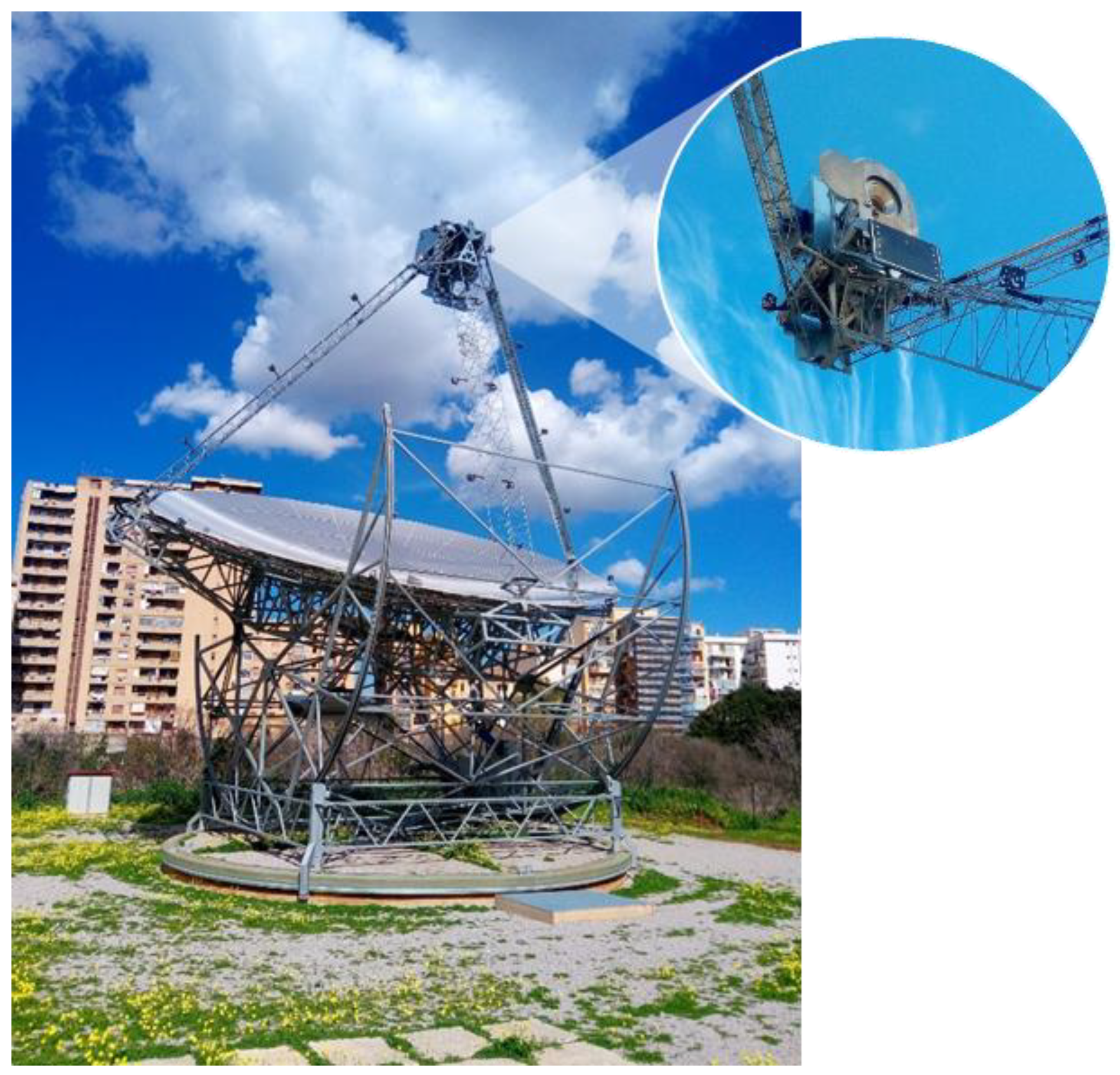
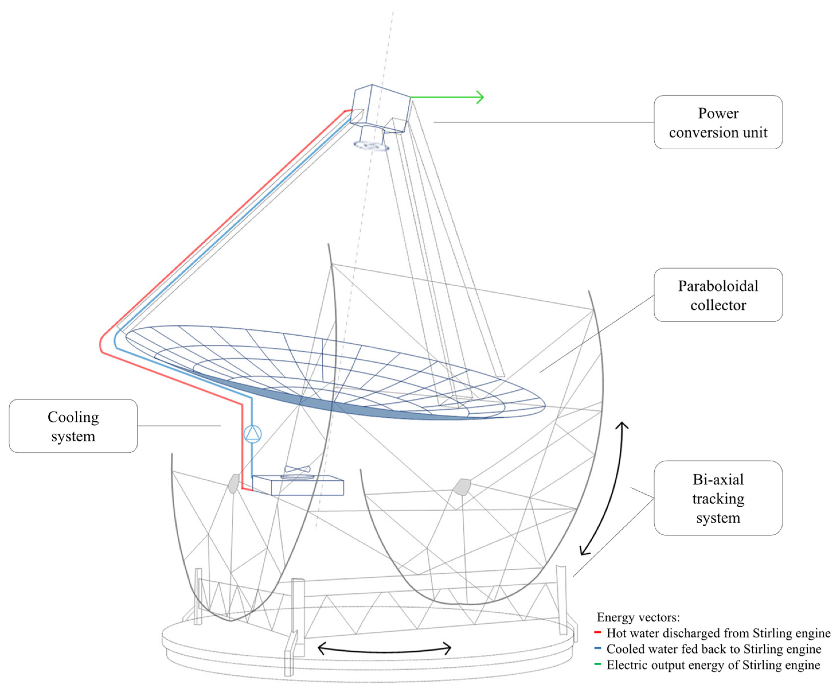
This paper proposes a neural approach to predict the electric energy production of a dish–Stirling solar concentrator at a specific, selected installation site. The reference system that is considered for the development of a neural prediction model is the demo commercial dish–Stirling solar concentrator installed on the university campus in Palermo (see Figure 1) as well as its real operational data.

This dish–Stirling plant has a net peak electric output power of 33 kW_e and features a geometric concentration ratio equal to 3217 (see

Table 1. Main technical parameters of the dish–Stirling system.

Parameter	Value	Unit
Paraboloidal reflector
Net aperture area of the dish collector ($A_n$)	106	m²
Aperture area of the receiver ($A_r$)	0.0314	m²
Focal length	7.45	m
Geometric concentration ratio	3217	-
Reflectivity of clean mirrors ($\rho$)	0.95	-
Power conversion unit
Peak electric output (DNI equal to 960 W/m²)	31.5 @ 2300 rpm	kWe
Type of Stirling engine	4 cylinders double acting
Displaced volume	4 (95 × 10−6)	m³
Max operating pressure of hydrogen	20	MPa
Temperature of the receiver ($T_r$)	720	°C

). The reference system has a paraboloidal collector consisting of an assembly of 54 mirrors with a high reflection coefficient; each mirror is characterised by a sandwich structure and a double curvature calibrated in order to concentrate the incident DNI on a fixed point corresponding to the small aperture of the cavity receiver. Subsequently, the Stirling engine and the electric generator convert the thermal energy into mechanical power and then electricity [34]. The power conversion unit (see zoom in Figure 1), including the receiver, the Stirling engine, and the electric generator, is placed at the focal point of the paraboloidal collector by a tripod.

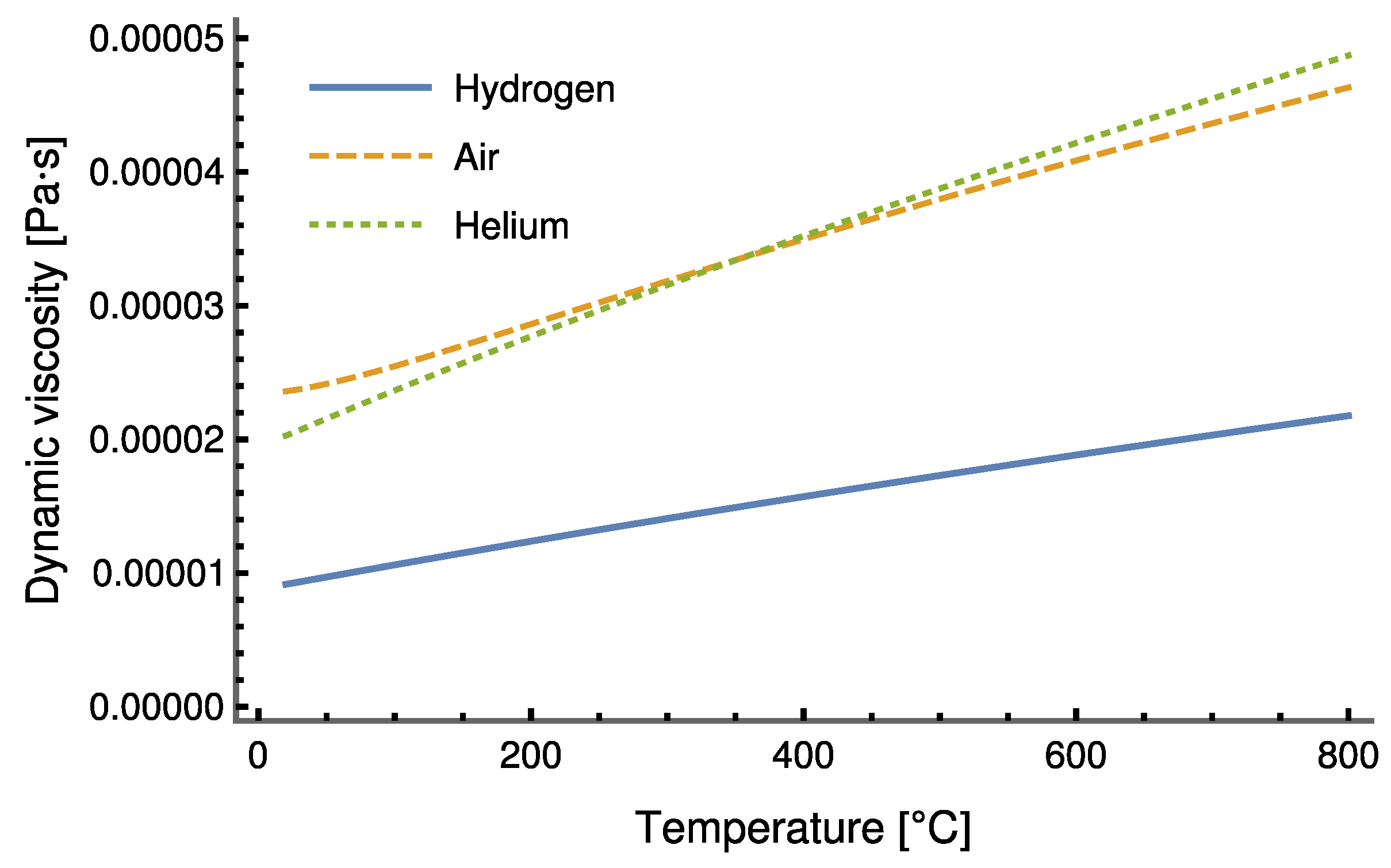
Inside the Stirling engine, hydrogen is used as the working fluid; the fundamental reason why hydrogen is selected as the working fluid is to minimise internal losses due to viscous friction. Figure 2 shows a comparison with two other possible fluids, air and helium, under the same working conditions. It is evident that hydrogen is less viscous than the other fluids considered. The curves drawn in Figure 2 were produced using the well-known database of thermodynamic properties provided by [35].

Moreover, the perfect alignment between the focal axis of the collector and the direction of the sun’s rays is ensured by a biaxial solar tracking system throughout the day [34].

3.1. Description of the Experimental Dataset

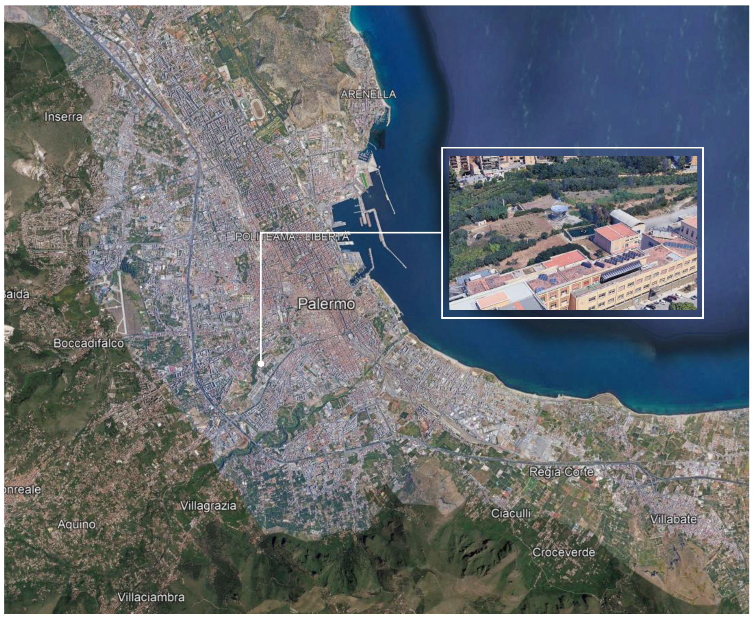
The installation site of the plant, on the outskirts of Palermo (see Figure 3), is characterised by typically Mediterranean climatic conditions. In this location, winters are generally characterised by very moderate temperatures ranging from 8 to 14 degrees. The summer period typically features rather high temperatures, sometimes even reaching 45 °C. Throughout most of the year, hot south-easterly winds, known as Sirocco winds, occur sporadically. Usually, the Sirocco winds bring with them a large amount of dust or sand from the North African coast, which tends to adhere to the external surfaces, strongly decreasing the amount of DNI available on the ground and, at the same time, decreasing the reflective properties of the mirrors of CSP systems.

The geographical coordinates specifying the installation site of the reference dish–Stirling system (described in Section 2) are long. 13°20′43″ E and lat. 38°06′17″ N.

All variables observed and recorded by the monitoring systems of the CSP plant are listed in

Table 2. All monitored variables of the CSP system.

Parameter	Description	Unit
Direct normal irradiance	Direct normal solar radiation incident per unit area by the reflector	W·m−2
Global horizontal irradiance	Global solar radiation incident per unit area by the reflector	W·m−2
Diffuse horizontal irradiance	Diffuse solar radiation incident per unit area by the reflector	W·m−2
Ambient temperature	Outdoor air temperature	°C
Average wind speed	Average wind speed on site	m·s−1
Wind speed	Wind speed on site	m·s−1
Wind direction	Wind direction on site	degree
Humidity	Relative humidity of external air	%
Air pressure	Outdoor air pressure	mbar
Solar azimuth	Instantaneous position of the sun relative to the south direction	degree
Solar elevation	Instantaneous position of the sun relative to the horizontal plane	degree
Total CSP net power output	Instantaneous power output of CSP less parasitic consumption	W

.

The index of cleanness (${\eta }_{cle}$) is a measure of the amount of soiling or dirt deposited on the reflector compared to the condition of clean mirrors, and, along with the reflectivity of mirrors ($\rho$), the interception factor ($\gamma$) of the concentrator (which is defined as the fraction of rays incident upon the aperture that reaches the receiver for a given incidence angle) and the absorption coefficient ($\alpha$) of the inner surface of the cavity receiver affect the optical efficiency (${\eta }_o$) of the CSP system (see Equation (1)) [18,36].

$${\eta }_o=\rho \cdot {\eta }_{cle}\cdot \gamma \cdot \alpha$$

(1)

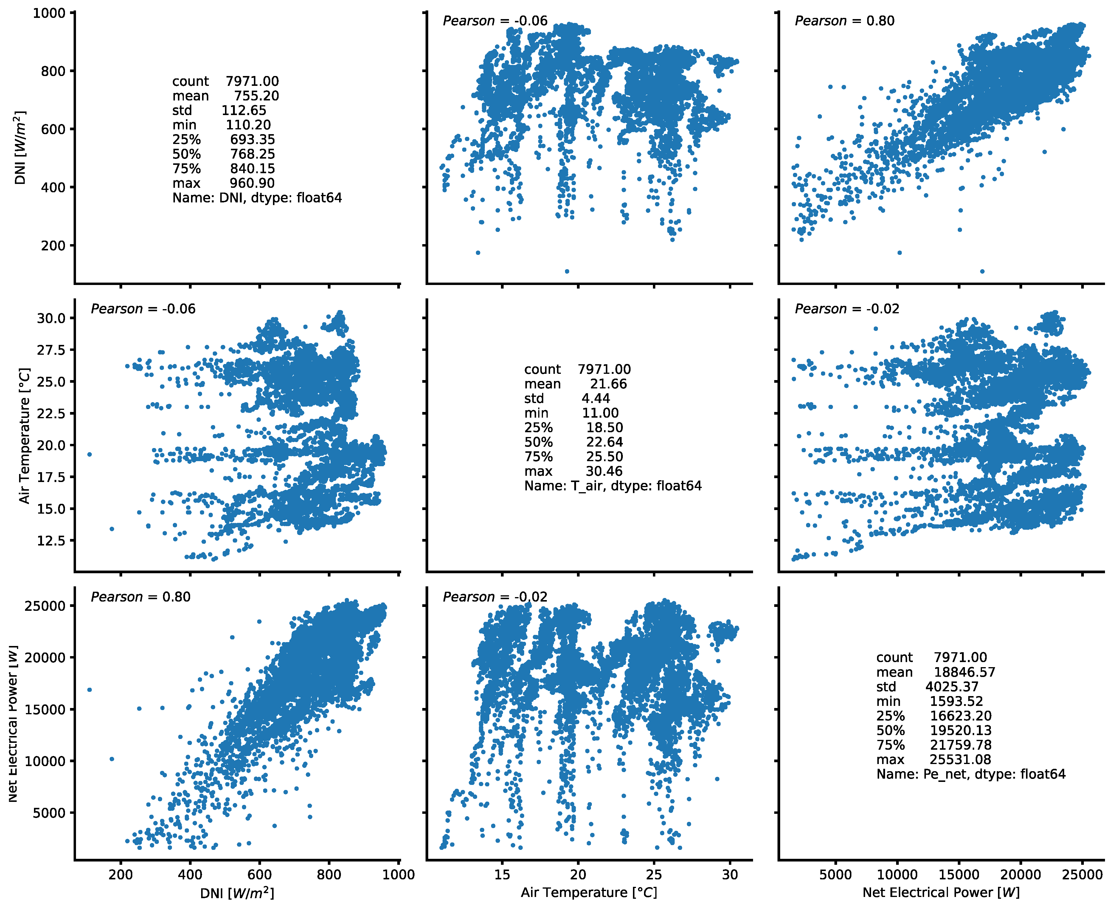
For the 165 days from 5 January 2018 to 2 July 2018, the monitoring system acquired 14,256,000 records (on a second-by-second basis). A large proportion of these records related to events when the plant was not operating because they corresponded to the night periods or day periods affected by weather conditions that were unsuitable for plant operation or to periods when the plant was under maintenance. The records relating to the remaining events were further aggregated with a simple average operation by single minutes, thus, we obtained 7971 records (data on a minute basis). 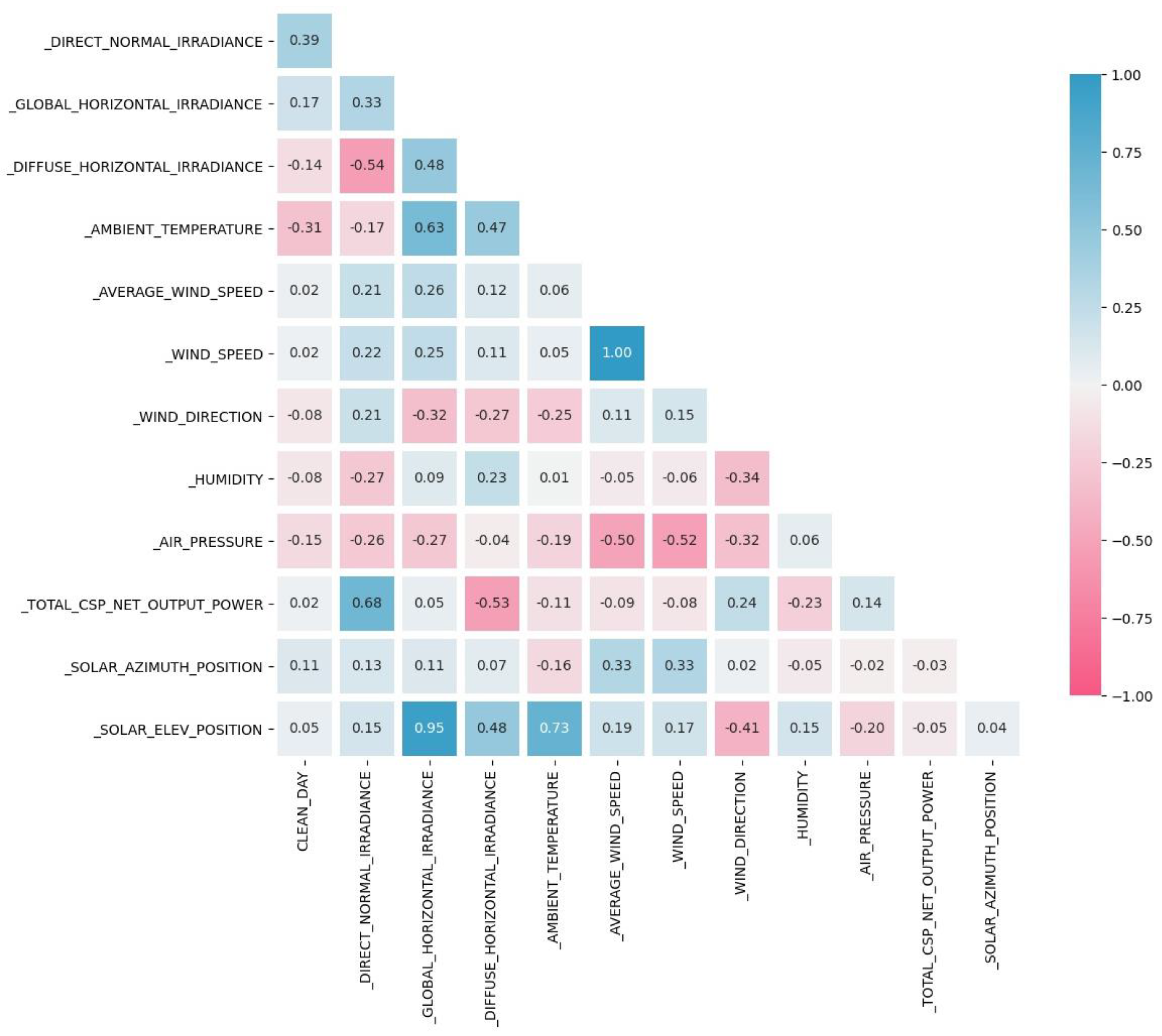Figure 4 shows some results of the statistical analysis carried out on those variables of the original dataset which, from a physical and thermodynamic point of view, are the most relevant to the operation of an engine based on a Stirling cycle. From a physical and thermodynamic point of view, the variables that are certainly most significant in determining the performance of a dish–Stirling system are the DNI, on which the power input to the system depends, and the outside air temperature, which affects, on the one hand, the heat exchange between the receiver and the external environment and, on the other hand, the heat exchange between the cold side of the Stirling engine and the environment. The Pearson coefficient (ρ_p) illustrated in Figure 5 shows that the net electrical power output of the dish–Stirling system is strongly correlated with the DNI.

3.2. Outlier Removal Procedure

As is usually the case, any population of samples or data can exhibit large deviations, meaning anomaly points or individual data points that deviate significantly from the rest of the distribution data. These data points are called outliers. The presence of outliers in a dataset can be due to a variety of factors, such as the experimental nature of the same data, human or measurement instrument errors, or wrong data handling; therefore, they are considered normal. In order to prevent outliers in the dataset from affecting the performance of any model developed, it is common practice to preliminarily identify and remove them to reduce the variability of the input dataset. Outliers can be either univariate or multivariate, depending on whether it is possible to identify them by observing a distribution of values in a single-dimensional space or an n-dimensional space. Obviously, in the latter case, the removal of outliers requires the training of an appropriate model able to replace the human brain. Several techniques are useful for detecting outliers in a dataset, of which the most widely used is the Z-score. The Z-score method uses standard deviation to identify outliers in a dataset with a Gaussian distribution (or those where the distribution is assumed to be Gaussian). Such a statistical quantity is a measure of how the observed data deviate from the most probably occurring data in the dataset, in other words, the mean of the data [37]. Referring to a Gaussian distribution of the data, the standard deviation ($\sigma$) is defined as in Equation (2) below:

$$\{\begin{array}{l}\sigma =\sqrt{\frac{{\displaystyle \sum _{i=1}^N{\left(x_i-\overline{x}\right)}^2}}{N-1}}\\ \overline{x}=\frac{1}{N}{\displaystyle \sum _{i=1}^N{x}_i}\end{array}$$

(2)

where $N$ is the number of records in the dataset, $x_i$ is the i-th record in the dataset, and $\overline{x}$ is the mean of the data (see Equation (2)). Thus, the Z-score ($z$) can be calculated by Equation (3) as:

$$z=\frac{x_i-\overline{x}}{\sigma }$$

(3)

In our case, the Z-score technique was applied considering three variables from the dataset, which were: the DNI, the net electric output power, and the outdoor air temperature. This is because, according to our experience of running the solar power plant installed at the Palermo University campus, these variables are the ones that most influence the behaviour of the system and can also vary very quickly. It should also be noted that abrupt variations can induce operating transients that can lead to system shutdown or restart within seconds. According to the Gaussian distribution of the data, all records falling within the range of extremes $\pm 2\sigma$ were considered. The resulting filtered dataset included 7417 records, approximately 93% of the originally available, valid data.

3.3. Statistical Analysis of Input Datasets

To describe and define the dataset, purified of outliers, a statistical analysis was carried out, investigating the quantities that are listed and explained in

Table 3. Summary of all used statistical quantities.

Statistical Quantity	Description	Formula
Arithmetic mean	the sum of a set of values divided by the number of values in the set	Equation (2)
Variance	measures how much a set of values quadratically deviates from its arithmetic mean	${\sigma }^2=\frac{1}{N}{\displaystyle \sum _{i=1}^N(}{x}_i-\overline{x}{)}^2$
Standard deviation	a measure of how much a set of values deviates from its arithmetic mean	Equation (2)
Standard error	a measure of how much the sample statistic (i.e., sample mean) deviates from the actual population mean	$se=\frac{\sigma }{\sqrt{N}}$
Skewness	a measure of the asymmetry of the probability distribution of the data	$\frac{N}{(N-1)(N-2)}\frac{1}{{\sigma }^3}{\displaystyle \sum _{i=1}^N(}{x}_i-\overline{x}{)}^3$
Kurtosis	a measure of the thickness of tails or the flattening of a probability distribution	$\frac{(N+1)N}{(N-1)(N-2)(N-3)}\frac{{\displaystyle \sum _{i=1}^N(}{x}_i-\overline{x}{)}^4}{{\sigma }^4}-3\hspace{0.17em}\frac{{(N-1)}^2}{(N-2)(N-3)}$

. These quantities were calculated for each variable of the original dataset without outliers, which included 7417 records, and were analysed by using the statistical variables summarised in Table 3 below.

The results of the preliminary statistical analysis of the data, summarised in

Table 4. Summary of all used statistical quantities.

Variable	Max Value	Arithmetic Mean	Variance	Standard Deviation	Standard Error	Skewness	Kurtosis
Clean day	131	46.61	1533	39.15	0.45	0.74	−0.95
Direct normal irradiance (W/m²)	957.17	774.63	7399.4	86.02	0.99	−0.14	−0.75
Global horizontal irradiance (W/m²)	1118	765.95	27869	166.44	1.94	−0.73	−0.49
Diffuse horizontal irradiance (W/m²)	512.2	157.06	4022.8	63.43	0.73	1	1.85
Ambient temperature (°C)	30.46	21.77	18.93	4.35	0.05	−0.26	−1.12
Average wind speed (m/s)	10.29	2.87	1.76	1.33	0.01	1.12	2.94
Wind speed (m/s)	11.43	3.13	2.08	1.44	0.02	1.23	3.38
Wind direction (deg)	340.65	145.32	5576.3	74.67	0.87	0.94	−0.59
Humidity (%)	71	52.15	90.45	9.51	0.11	−0.19	−1.06
Air pressure (hPa)	1026.1	1006.7	34.85	5.90	0.06	0.57	1.87
Solar azimuth (deg)	265.05	167.99	2512.3	50.12	0.58	0.17	−1.20
Solar elevation (deg)	75.42	54.04	217.07	14.73	0.17	−0.35	−1.05
Total CSP net power output (W)	25531	19516	9.65 × 106	3107.8	36.08	−0.36	−0.63

, describe the main characteristics of the data and provide precise quantitative information on the data distribution, variability, skewness, and taililedness of the actual data sample available to the authors. The analysed data sample refers to all monitored variables listed in Table 2 and to the variable “Clean day”, which indicates the number of days since the last cleaning event affecting the mirrors.

The full input dataset of 7417 samples was always randomly split to obtain an input dataset for the training process of the neural networks and another input dataset to be used for the validation process of the same neural networks; the training dataset included 85% of the original data; the validation dataset resembles the other 15%. Preliminary statistical analysis of the data made it possible to evaluate the correlation coefficients between each of the variables covered, and the results are exemplified by Figure 5.

To avoid any form of direct influence or manipulation in order to improve the predictive performance of the developed neural models, training and validation datasets were autonomously extracted by the software in random mode from the set of data monitored on our prototype system. Therefore, no filter or algorithm was applied for the above splitting operation except for that used for the removal of outliers. In this sense, punctual data used for the training of the network were never used to validate the results and vice versa. Although, in theory, point data might be used for the training phase, and the one immediately following in time used for validation, it is necessary to underline that we did not applied algorithms specifically indicated for time series. The data, before being used, were purposely remixed, eliminating any temporal succession. In addition, the operation of the dish–Stirling was characterised by extreme and fast variability due to a continuous variability of weather and solar parameters.

4. Energy Modelling of the Dish–Stirling Concentrator

As it is possible to observe from the layout of the plant depicted in Figure 6, the dish–Stirling solar concentrator is mainly composed of four subsystems [9], which are: the paraboloidal reflector; the power conversion unit, which includes all those components that provide energy conversion as well as the cavity receiver [38], the Stirling engine, and the electric generator [34]; the biaxial tracking system; and the cooling system of the engine [39].

The analytical energy model of dish–Stirling technology [18] most recently disseminated in the scientific literature was developed firstly using the energy balance of the system and was subsequently calibrated using experimental data from a single clear-sky day. This energy model allows the evaluation of the net electric output power of the dish–Stirling system as a function, essentially, of three quantities: the DNI, the ambient air temperature, and the level of cleanliness of the mirrors.

Energy and Heat Balance Equations

The development of the analytical energy model of the dish–Stirling system, to which reference is made, was based on the energy and heat balance of the same system [18]. The flow chart in Figure 7 indicates the energy input and output rates affecting the various subsystems of the dish–Stirling solar concentrator.

The solar power input to the paraboloidal reflector is the result of DNI intercepting the aperture area of the collector. However, this power is not fully available to the receiver because part of this power is lost to the environment due to optical inefficiencies in the system. In addition, the receiver is also affected by thermal losses due to the temperature difference between the cavity and the environment.

The thermal power (${\dot{Q}}_{r,out}$) lost at the receiver is due to the combined effect of radiative and convective heat transfer to the environment, and it can be calculated using Equation (4):

$${\dot{Q}}_{r,out}=A_r\cdot \left\{{\mathrm{h}}_r\cdot \left(T_r^{ave}-T_{air}\right)+{\sigma }_{SB}\cdot {\epsilon }_r\cdot \left[{\left(T_r^{ave}+273.15\right)}^4-{\left(T_{sky}+273.15\right)}^4\right]\right\}\left[\mathrm{W}\right]$$

(4)

where:

• $A_r$ is the aperture area of the cavity receiver (m²);
• $h_r$ is the convective heat transfer coefficient of the receiver (W/(m²∙K));
• $T_r^{ave}$ is the average value of the receiver temperature (°C);
• $T_{air}$ is the temperature of the external air (°C);
• ${\sigma }_{SB}$ is the Stefan–Boltzmann constant equal to 5.67∙108 W/(m²∙K4);
• ${\epsilon }_r$ is the emissivity of the cavity receiver (-);
• $T_{sky}$ is the sky’s apparent temperature calculated using the empirical formula [40] of Equation (5):

  $$T_{sky}=0.0552\cdot {\left(T_{air}+273.15\right)}^{1.5} - 273.15\left[°\mathrm{C}\right]$$

  (5)

Despite these losses, the thermal power that the receiver transfers to the hot side of the Stirling engine (${\dot{Q}}_{S,in}$) is converted into mechanical energy at the engine crankshaft (${\dot{W}}_S$) thanks to the working fluid (hydrogen), which evolves according to the homonymous thermodynamic cycle. The analytical energy model [18] uses a linear correlation to relate these last two quantities. Thus, the mechanical power output of the Stirling engine (${\dot{W}}_S$) can be calculated using Equation (6) as follows:

$${\dot{W}}_S=\left(a_1\cdot {\dot{Q}}_{S,in}-a_2\right)\cdot R_T[\mathrm{W}]$$

(6)

where:

• $a_1$ (-) and $a_2$ (W) are two fitting parameters of the mechanical efficiency curve of the Stirling engine;
• $R_T$ is a dimensionless correction factor of the ambient air temperature ($T_{air}$) for the reference temperature ($T_0$ set equal to 25 °C) (both expressed in °C) defined as:

  $$R_T=\frac{T_0+273.15}{T_{air}+273.15}$$

  (7)

The final energy conversion step is carried out by the electric generator. Lastly, excluding the parasitic absorption of electric power by the engine cooling system and the solar tracking system, the net electrical power produced by the dish–Stirling system (${\dot{E}}_n$) can be expressed by Equation (8) as follows:

$${\dot{E}}_n\left(I_b,\hspace{0.17em}{T}_{\mathrm{air}},\hspace{0.17em}{\eta }_{cle}^{ave}\right)={\eta }_e\cdot R_T\cdot \left[a_1\cdot \left({\eta }_o\cdot {\eta }_{cle}^{ave}\cdot I_b\cdot A_n-{\dot{Q}}_{r,out}\right)-a_2\right]-\hspace{0.17em}{\dot{E}}_p^{ave}[\mathrm{W}]$$

(8)

where:

• $I_b$ is the DNI arriving on the mirrors (W/m²);
• $T_{air}$ is the ambient air temperature (°C);
• ${\eta }_{cle}^{ave}$ is the average level of cleanliness of the mirrors, ranging between 0 and 1 (-);
• ${\eta }_e$ is the mechanical-to-electric conversion efficiency of the electric generator (-);
• ${\eta }_o$ is the optical efficiency of the solar concentrator (-);
• $A_n$ is the net aperture area of the paraboloidal collector (m²);
• ${\dot{Q}}_{r,out}$ is the thermal power loss at the cavity receiver (W);
• ${\dot{E}}_p^{ave}$ is the average value of electric power consumed by parasitic equipment, such as the tracking system and dry cooler of the cooling system (W).

The values of the main parameters used as input to the analytical model described above are reported in

Table 5. Main parameters used as input to the analytical model of the dish–Stirling system of Palermo.

Parameter	Value	Unit
Net aperture area of the collector ($A_n$)	106	m²
Aperture area of the cavity receiver ($A_r$)	0.0314	m²
Convective heat transfer coefficient of the receiver ($h_r$)	10	W/(m²∙K)
Emissivity of the cavity receiver (${\mathsf{\epsilon }}_{\mathrm{r}}$)	0.88	-
$a_1$ parameter	0.475	-
$a_2$ parameter	3319	W
Average receiver temperature (${\mathrm{T}}_{\mathrm{r}}^{\mathrm{a}\mathrm{v}\mathrm{e}}$)	720	°C
Average level of cleanliness of the mirrors (${\eta }_{cle}^{ave}$)	0.85	-
Electric efficiency of the PCU (${\eta }_e$)	0.924	-
Clean mirrors’ optical efficiency (${\eta }_o$)	0.85	-
Average electric power consumption (${\dot{E}}_p^{ave}$)	1600	W

.

Knowing the climate data characteristics of a location, e.g., those from a typical meteorological year (TMY), the energy model [18] can be used to assess the energy performance of the dish–Stirling system. Furthermore, in [41], based on this analytical energy model, a simple new algorithm was developed to evaluate the energy performance of the dish–Stirling system knowing only the hourly frequency distribution of the DNI of the installation site.

5. Artificial Neural Network Models

5.1. Machine Learning Deployment Using TensorFlow and Python

In recent years, the use of neural network technologies and algorithms applied to physical and engineering problems has become increasingly common, and software companies have made increasingly sophisticated tools available for analysing complex systems. However, such software often requires the user to have detailed knowledge of artificial intelligence, which has slowed the spread of these interesting methodologies. The cost of purchasing such software has been another limiting factor for the spread of machine learning techniques. The diffusion of open-source libraries characterised by high reliability and effectiveness has facilitated the success of this ground-breaking technology. In this context, Google’s TensorFlow 2 library represents an extremely powerful, free tool, which, at the same time, is characterised by extreme ease of use for the production of machine learning algorithms in several programming environments [42]. For the development of the models described below, the authors used the Python code language, which is very well suited to some of the particular functionalities of TensorFlow 2 [43], such as saving and restoring the state of a neural network in order to predict at a time following the training of the network itself [44]. Python is a programming language, developed in the 1990s, that is particularly suited to the development of applications that rely on numerical computation. It is free of charge and is available for a wide range of operating systems, a feature that has made it particularly popular in academic circles [45,46]. All the machine learning models described below, therefore, use libraries and environments that are completely free and reusable for absolute transparency and replicability of the results.

5.2. Artificial Neural Networks

The artificial neural network (ANN) is a powerful tool, the sophisticated rationale of which is inspired by the way the human brain analyses and elaborates information [47]. ANNs are largely used for the modelling, prediction, assessment, and optimisation of the performance of many different engineering technologies, such as solar energy systems, which often require the solving of complex and non-linear problems [48].

In this paper, from all the different types of ANNs, the multilayer perceptron (MLP) and the radial basis function (RBF) models were selected.

5.2.1. Multilayer Perceptron Neural Network

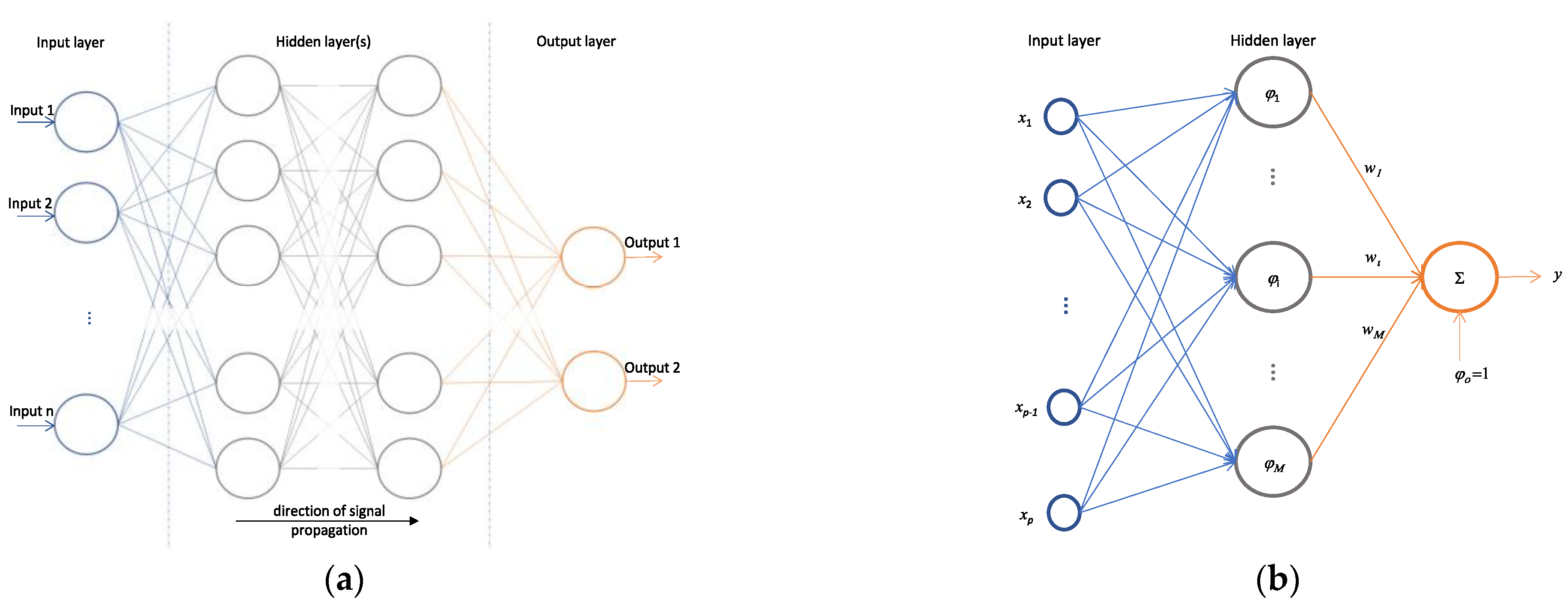
The MLP neural network (see Figure 8a) consists of several layers (an input layer, several hidden layers, and an output layer) in which the neurons are ordered to transmit signals from the input to the output of the network. The output (${\phi }_i\left(x\right)$) of each neuron of the hidden layer and the network output ($y$) are mathematically described by the following Equation (9):

$$\{\begin{array}{l}{\phi }_i\left(x\right)\hspace{0.17em}=\zeta \left({\displaystyle \sum _k{a}_{ik}{x}_k+b_i}\right)\hspace{0.17em}\\ y={\displaystyle {\sum }_i{w}_i{\phi }_i}\end{array}$$

(9)

where $\zeta$ is a non-linear function, $a_{ik}$ is the weight of the first layer, $x_k$ is the input information, $b_i$ is the bias, and $w_i$ is the weight of the output layer [48].

5.2.2. Radial Basis Function

As can be seen in Figure 8b, which shows the architecture of a general RBF network, each neuron of the hidden layer has a vector of parameters called centre ($x_i$), which is compared with the input vector ($x$) of the network, producing a radial, symmetric response [49]. The responses of the hidden layer are also scaled by the connection weights ($w_i$) to the output layer and then combined to generate the output of the network [50]. The output (${\phi }_i\left(x\right)$) of each neuron of the hidden layer and the network output ($y$) are mathematically described by Equation (10) as:

$$\{\begin{array}{l}{\phi }_i\left(x\right)\hspace{0.17em}=g\left(|x-x_i|\right)\\ y={\displaystyle {\sum }_i{w}_i{\phi }_i}\end{array}$$

(10)

where $g(.)$ can be a Gaussian function [48].

Keras layers are the basic building blocks of neural networks in Keras, the open-source framework used in our research. A layer consists of a tensor-in tensor-out computation function (the layer’s call method) and a state, held in TensorFlow variables (the layer’s weights). While Keras offers a wide range of built-in layers, it does not cover every possible use case. Indeed, a radial basis function layer was achieved by customising the already available layers in Keras [42,51].

5.3. Development of Neural Network Models

This section defines the models and the description of the neural network architectures, both MLP and RBF, which were used for the prediction of the energy producibility of the analysed dish–Stirling plant. As indicated in

Table 6. Input and output variables of datasets implemented in both MLP and RBF neural network models.

Long Dataset	Short Dataset
Input variables
Direct normal irradiance	Direct normal irradiance
Ambient temperature	Ambient temperature
Clean day
Global horizontal irradiance
Diffuse horizontal irradiance
Average wind speed
Wind speed
Wind direction
Humidity
Air pressure
Solar azimuth
Solar elevation
Output variables
Total CSP net power output	Total CSP net power output

, for both types of ANN models, the total net output power of the CSP was the only output variable of the networks, and two different datasets were defined for the input variables to these same networks; the first included twelve variables (long dataset), and the second one included only two variables (short dataset). It is important to highlight that the identification of a restricted group of variables, to be used in the training phase, was carried out after a preliminary sensitivity analysis of the energy performance of the plant with respect to the environmental and operating conditions of the technology, also taking into account the physical features of the phenomena occurring in a CSP plant such as the one being investigated.

Two possible types of input datasets are presented in the research described here: long and short. The long dataset consisted of all significant variables made available by our monitoring system. The short dataset, on the other hand, considered only the two climate variables that are absolutely necessary from the physical point of view to describe the energy balance and the related analytical model of the dish–Stirling system. The two possible datasets, therefore, delimit the widest interval within which the input variables can be selected.

For both MLP and RBF models, several neural network architectures characterised by different levels of depth were tested for each of the two datasets of variables defined. Specifically, the performance of each network architecture was investigated for four different depth levels, varying the number of neurons in the layers and the number of layers making up the neural network. Therefore, a total of 16 networks were trained, of which eight were of the MLP type, and the other eight were of the RBF type.

From this point on, for ease of writing and to better identify the different neural networks examined, each of them is associated with the nomenclature X-Y-N, in which: X is a letter that indicates the level of depth of the network, which can be superficial (S), medium deep (M), deep (D), or very deep (V); Y is an acronym that can be MLP or RBF depending on the type of neural network implemented; and N is a number that can be equal to 2 or 12 depending on how many input variables were used.

Table 7. Input and output variables of datasets implemented in both MLP and RBF neural network models.

ANN Code	Number of Layers	Neurons	Trained Parameters
S-MLP-2	4	2 + 20 + 5 + 1	181
S-MLP-12	4	12 + 50 + 10 + 1	1351
S-RBF-2	4	2 + 20 + 5 + 1	181
S-RBF-12	4	12 + 50 + 10 + 1	1351
M-MLP-2	4	2 + 40 + 20 + 1	971
M-MLP-12	4	12 + 150 + 30 + 1	6691
M-RBF-2	4	2 + 40 + 20 + 1	971
M-RBF-12	4	12 + 150 + 30 + 1	6691
D-MLP-2	5	2 + 140 + 300 + 80 + 1	66,891
D-MLP-12	5	12 + 140 + 300 + 80 + 1	68,461
D-RBF-2	5	2 + 140 + 300 + 80 + 1	66,891
D-RBF-12	5	12 + 140 + 300 + 80 + 1	68,461
V-MLP-2	8	2 + 130 + 200 + 400 + 700 + 100 + 50 + 1	462,897
V-MLP-12	8	12 + 130 + 200 + 400 + 700 + 100 + 50 + 1	464,371
V-RBF-2	8	2 + 130 + 200 + 400 + 700 + 100 + 50 + 1	462,901
V-RBF-12	8	12 + 130 + 200 + 400 + 700 + 100 + 50 + 1	464,371

summarises the main characteristics of all 16 neural networks tested to predict the energy producibility of the dish–Stirling plant, reporting for each network: the number of layers, the number of neurons in each layer, and the total number of parameters involved in the training process.

5.4. Description of Supplementary Materials

The programming language used to build the artificial neural network models defined in Table 7 was Python employing TensorFlow libraries. Supplementary Materials include all scripts and data necessary to ensure the complete replicability of the neural network models examined and proposed for predicting the electrical producibility of a dish–Stirling system. Among them, the master script defines the network architecture of the neural model (see ‘NN_script.py’), and the reader can examine it to recreate, modify, and review the modelling procedures and data used in both the training and validation phases. With regard to the input data of the neural networks examined, although the complete original dataset is not provided due to confidentiality issues, a limited dataset used for the validation phase of the neural networks is nevertheless provided both for the long input dataset, which includes twelve variables (see ‘y_test.txt’), and for the short input dataset, which includes two variables (see ‘X_test.txt’). Various strategies were used to avoid overfitting, involving the definition of different checkpoints. The checkpoint configures the early stopping of the training phase in order to avoid overfitting by using a measure of the loss of accuracy in the validation phase and setting a maximum number of training repetitions (epochs) for which no improvement in the accuracy of the prediction is detected.

Finally, a simplified script is provided (see “NN_reload_script.py”), which allows the user to instantly execute the best neural network by reading a file in which all the parameters of the best neural network are stored (see “best_dish_model_achieve.h5”). This set of files allows the user to directly verify the results of the present study and possibly modify and reuse these architectures even in other cases.

5.5. Definition of Performance Measures

With the aim of assessing the quality and reliability of the neural models developed, several statistical indices were calculated, starting from the validation dataset, including the determination coefficient R squared explained by Equation (11) in

Table 8. Statistical quantities calculated on residuals.

Statistical Index	Symbol	Formula
Coefficient of determination	R²	$1-\frac{{\displaystyle {\sum }_i{e}_i^2}}{{\displaystyle {\sum }_i{\left(y_i-\mu \right)}^2}}$ (11)
Mean absolute error	MAE	$\frac{{\displaystyle {\sum }_{i=1}^C\left|y_i-m_i\right|}}{C}$ (12)
Count	C	Size of the validation dataset
Mean	$\mu$	$\frac{1}{C}{\displaystyle \sum _{i=1}^C{e}_i}$
Standard deviation	$\sigma$	$\sqrt{\frac{{\displaystyle \sum _{i=1}^C{\left(e_i-\overline{e}\right)}^2}}{C-1}}$
Minimum	min	min($e_i$)
Maximum	max	max($e_i$)
Quartile at 25%	Q1	Value for which the cumulative percentage frequency of the sample is at least 25%
Quartile at 50%	Q2	Value for which the cumulative percentage frequency of the sample is at least 50%
Quartile at 75%	Q3	Value for which the cumulative percentage frequency of the sample is at least 75%

, which provides a synthetic measure of the goodness of the approximate function. This index can assume a value between 0 and 1 and indicates how far the predicted values deviate from the expected ones. Moreover, starting from the validation dataset again, the mean absolute error (MAE) was produced for each trained neural network. The MAE, explained in Equation (12), is the average of the absolute differences between the prediction and the actual value of the output variable of the neural network, providing information on the average magnitude of errors in a set of predictions, regardless of their direction.

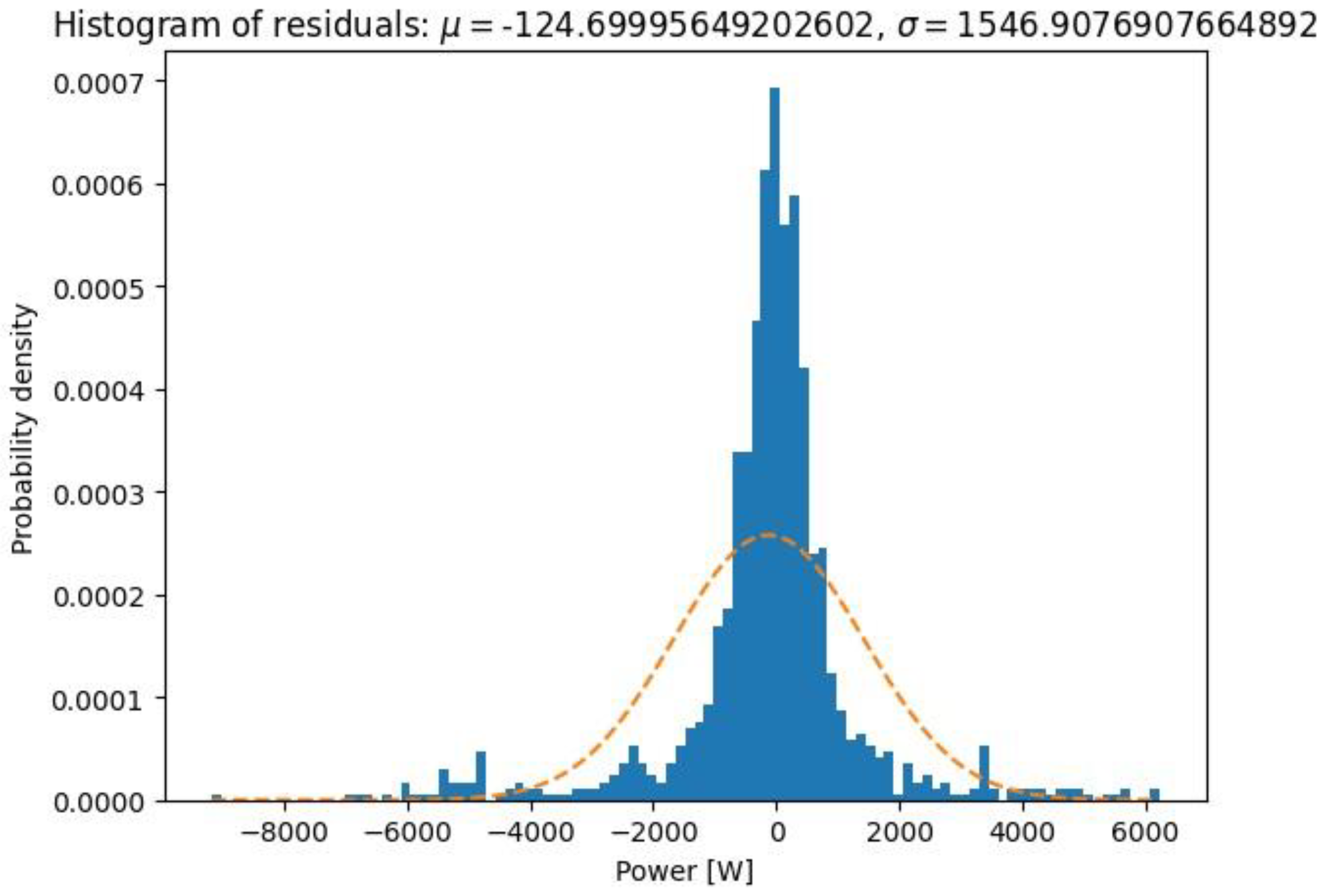
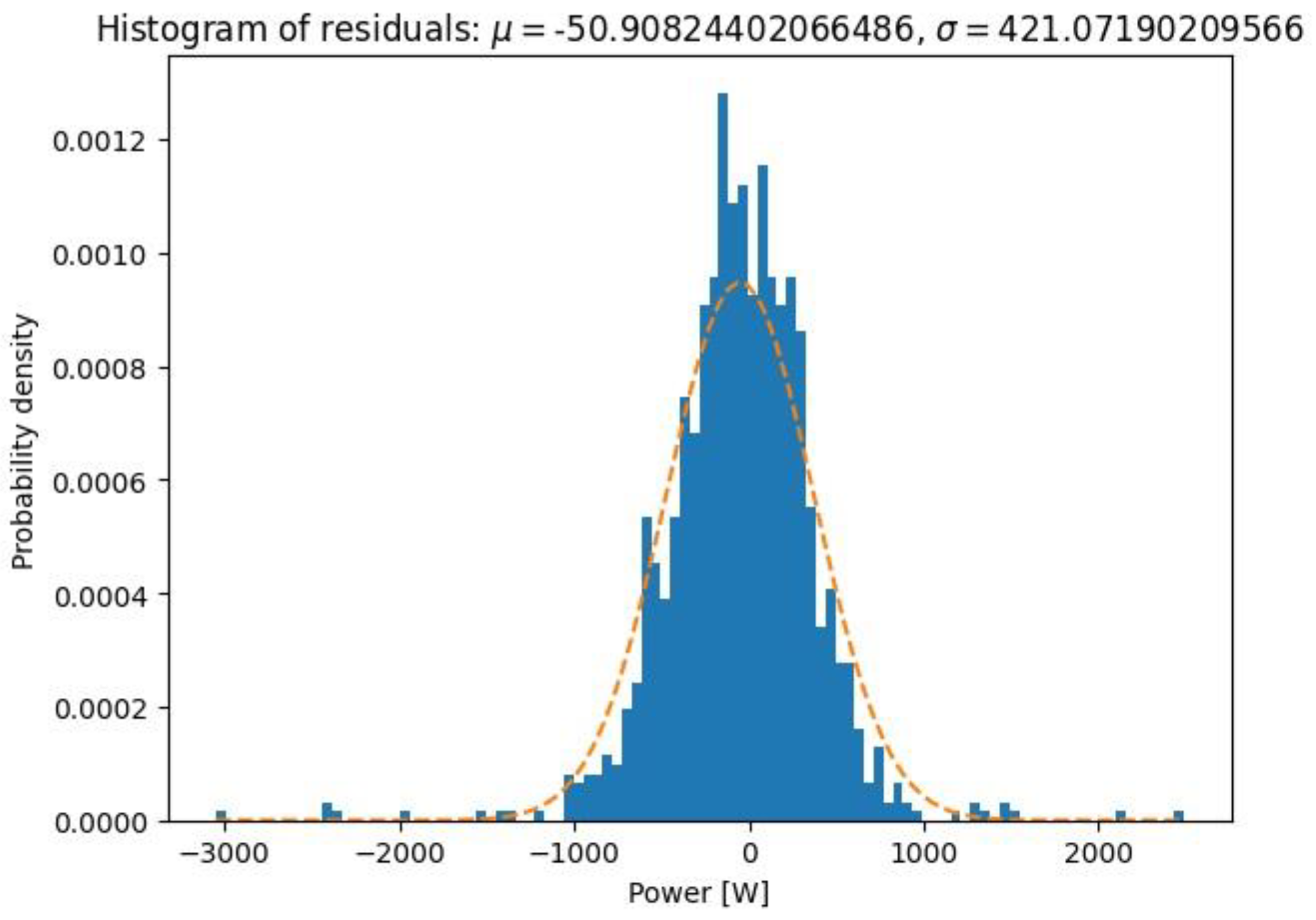
In addition, a statistical analysis of the resulting residuals was carried out after the validation process for each neural network. Being residuals ($e_i$), the set of differences was obtained by subtracting the actually measured values from those predicted as the output variable of the networks. The following quantities were then evaluated to examine the frequency distribution of these residuals, such as the mean value, the size of the validation dataset (count), the standard deviation value, the minimum and maximum values, and quartiles at 25% (first quartile, Q₁), at 50% (second quartile, Q₂), and 75% (third quartile, Q₃). In order to graphically compare all the developed neural networks in terms of the accuracy of predicting the energy production of the dish–Stirling plant, the following graphs were produced for each of them:

(1) A histogram of residuals showing the distribution of residuals obtained by comparing the values of the electrical output power of the dish–Stirling system predicted against that measured. From this comparison, the mean ($\mu$) and standard deviation ($\sigma$) values of the residuals were calculated and displayed. In general, it is expected that the distribution is centred on the value 0 and is close to a Gaussian distribution. However, in this graph, it is also possible to graphically compare the probability density distribution obtained with a normal distribution having the same mean value and the same standard deviation value;

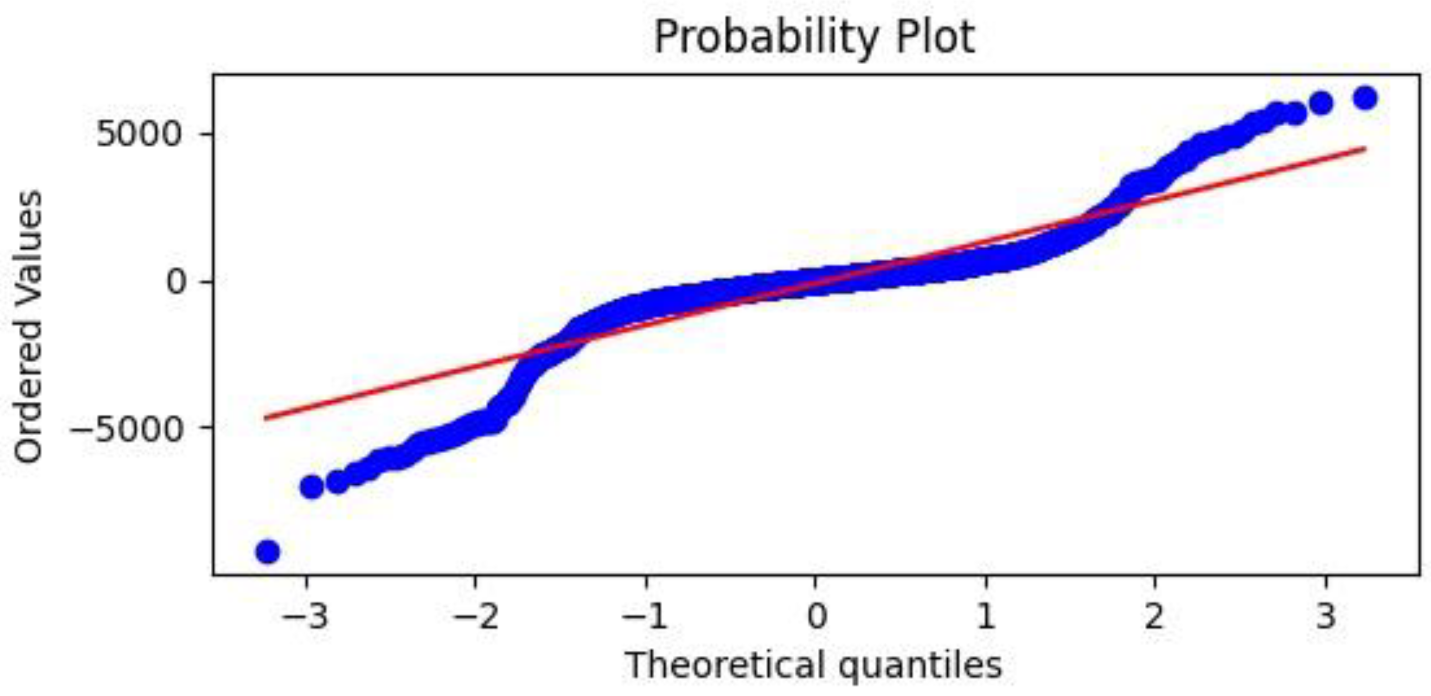
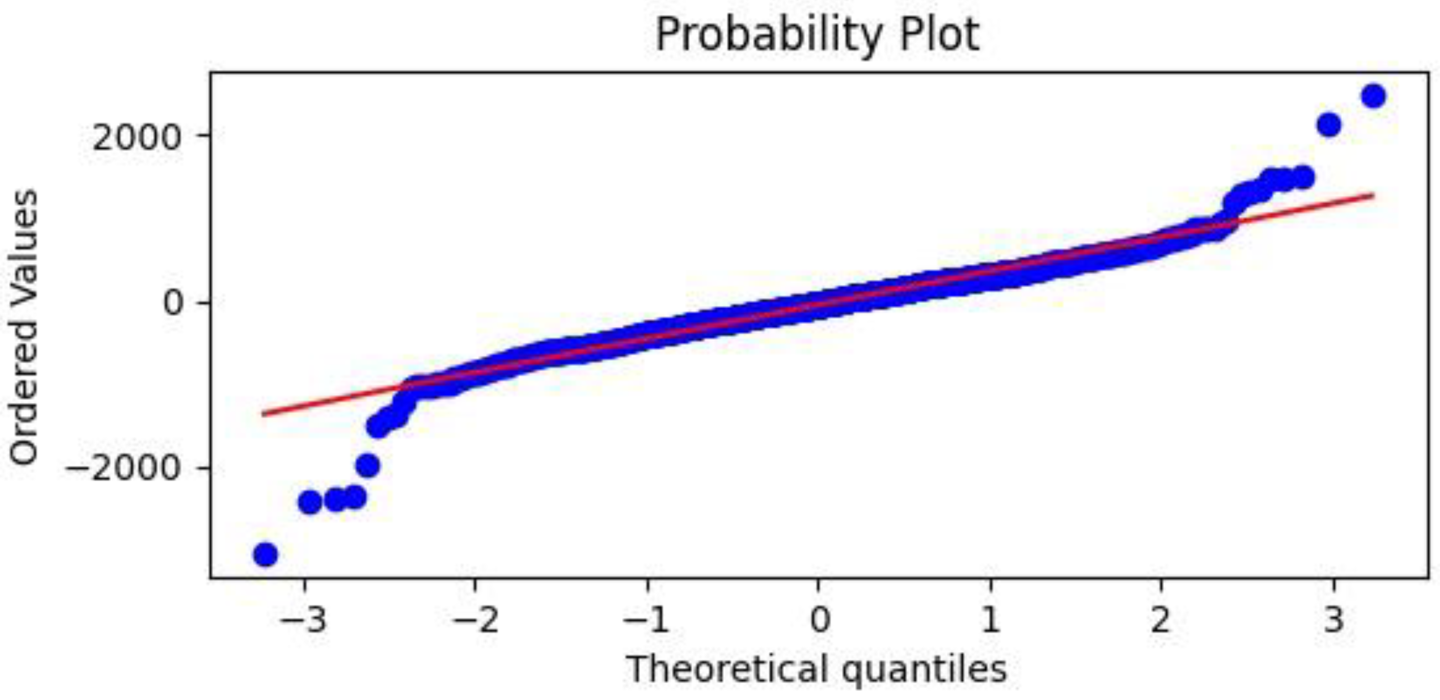
(2) A Q–Q (quantile–quantile) plot, a probability plot in which the probability distributions of the residuals obtained after the validation process are compared with a normal distribution by plotting their quantiles against each other;

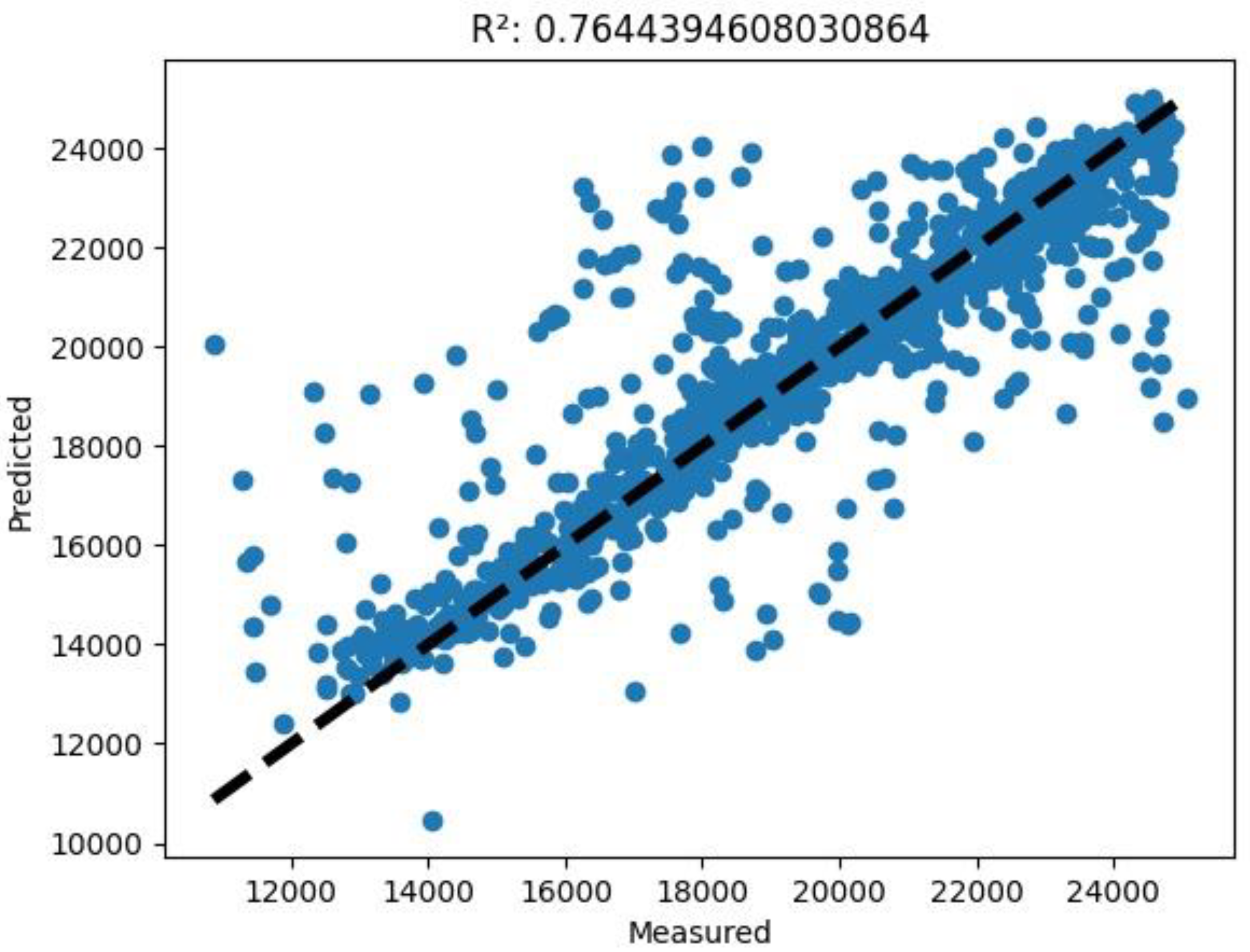
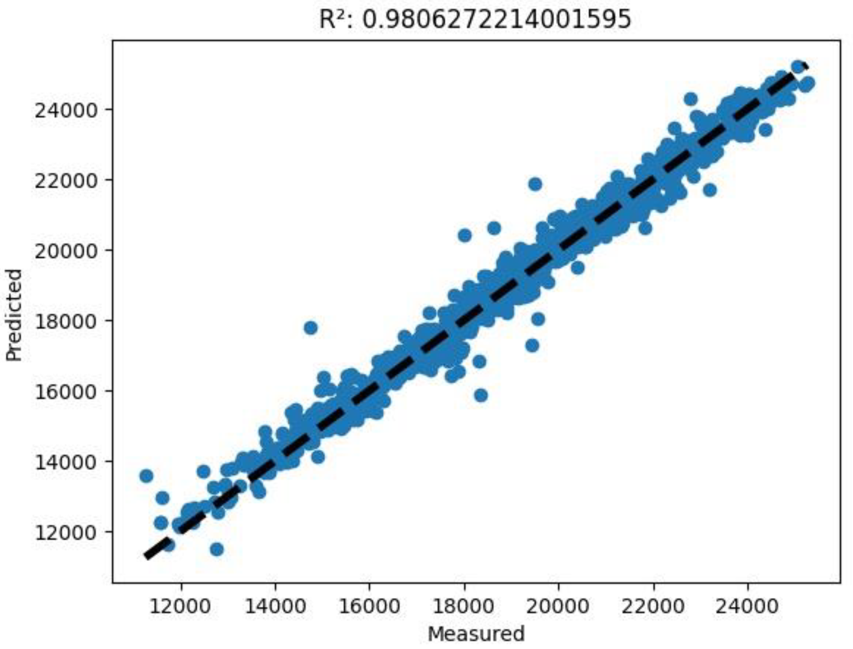
(3) A predicted versus measured graph showing points of coordinates expected and actual measured electrical output power values. In this graph, it is possible to appreciate, through the coefficient of determination R squared explained in Equation (11) (see Table 8), the spatial distribution of the points with respect to the bisector of the first quadrant, which represents an ideally perfect regression.

6. Results and Discussion

6.1. Performance of Neural Network Models

In general, in the scientific literature, when neural networks are used as function approximators, it is very common to use RBF-type architectures [49]. However, neural networks with MLP-type architecture are excellent function approximators because they can replicate any type of mathematical function [48]. As can be noted from

Table 9. Values of all statistical quantities calculated on residuals resulting from the validation process of all 16 neural networks tested.

ANN Code	R2	MAE	m	s	Min	Max	Q1	Q2	Q3
S-MLP-2	0.57	1597.8	−191.4	2038.6	−8113.1	5141	−11198.2	−22.4	1234
S-MLP-12	0.92	599.8	68.0	872.8	−4827.7	6164.7	−323.1	107.1	509.5
S-RBF-2	0.55	1650.5	7.4	2065.1	−6563.9	4908.6	−1320.3	173.2	1474.1
S-RBF-12	0.80	964.1	19.5	1341.9	−7987.8	8043.8	−630.6	46.7	705.9
M-MLP-2	0.63	1325.1	−148.2	1891.9	−8370.4	4382	−777.2	9.8	946.7
M-MLP-12	0.94	465.9	−5.5	720.8	−7290	3536.8	−281.3	59.5	390.9
M-RBF-2	0.62	1375.5	−250.7	1956.2	−8494.6	4800.2	−909.3	35.7	836.6
M-RBF-12	0.85	795.1	−62.9	1167.7	−5386.1	5695.8	−583.8	−44	451.2
D-MLP-2	0.72	1059.4	−99.4	1633.2	−7544.2	6653.0	−634.6	−17.8	576
D-MLP-12	0.95	419.7	−58.4	653	−6596.8	3117.6	−335	−21.1	285.7
D-RBF-2	0.70	1047.2	−39.3	1671.5	−7516.9	6034.8	−506.8	44.4	585.1
D-RBF-12	0.94	458.5	−87.1	695.7	−5627.9	6163.3	−362.4	−15.6	317.5
V-MLP-2	0.76	904.8	−124.6	1546.9	−9183.2	6220.4	−518.4	−28.1	385.2
V-MLP-12	0.98	306.9	−50.9	421	−3050.8	2484.5	−275.2	−45.0	205.4
V-RBF-2	0.73	936.2	91.7	1615.2	−8514.5	7946.0	−421.5	22.1	476.2
V-RBF-12	0.95	420	−66.7	682	−5950.3	7282.2	−353.6	−29.4	241.3

, which summarises all the statistical variables calculated to assess the prediction accuracy obtained by the 16 neural networks developed, the results show that the modelling approach through RBF did not prove to be the most efficient in this study. Conversely, neural networks based on an MLP-type architecture always led to better results, both when varying the level of depth of the network and when varying the number of input variables to the neural network.

Furthermore, for the same type of architecture (MLP and RBF) and the number of input variables, it can be seen from

Table 10. Training time and velocity of all 16 neural networks tested with an i7 CPU with 32 GB of RAM.

ANN Code	Elapsed Time (s)	Velocity (epochs/s)
S-MLP-2	1662	0.487
S-MLP-12	2607	0.500
S-RBF-2	711	0.555
S-RBF-12	454	0.603
M-MLP-2	1558	0.217
M-MLP-12	1221	0.300
M-RBF-2	1613	0.203
M-RBF-12	1074	0.458
D-MLP-2	1595	0.333
D-MLP-12	1215	0.341
D-RBF-2	2505	0.385
D-RBF-12	1662	0.480
V-MLP-2	15731	0.507
V-MLP-12	5848	0.506

that increasing the depth of the network, and, in parallel, increasing their complexity (in terms of the number of neurons), generally led to better performance but longer training times (see Table 9). For this reason, the authors did not consider it appropriate to experiment with even more complex network architectures.

Table 10 shows the total time it took to train the different models and the speed evaluated in training epochs per second. Furthermore, it is important to underline that too many input parameters can theoretically degrade the predictive performance of a neural network and require excessive computational resources. In order to consciously guide the reader in the choice of the number of input variables, we have, for the sake of the argument, provided in Table 10 the time required for the proper training of each neural model presented. Naturally, once properly trained, the networks are able to perform prediction virtually instantaneously. The reader can verify the variation of performance and time required for correct training by using and modifying the neural network architecture by downloading the configuration scripts and input datasets made available in “Supplementary Materials”.

The coefficients of determination (see R² in Table 9) calculated for the neural networks using synthetic input datasets (short datasets including two input variables) fell within a range of values between 0.55 and 0.76. On the other hand, the neural networks using 12 input parameters (long dataset of input variables), specifically including the variable providing the number of days since the last cleaning event of the reflecting mirrors (Clean day—see Table 6), allowed the achievement of much better results in terms of R squared, with values falling in the range between 0.80 and 0.98. Generally, the best performance-tested neural networks had the following codes: V-MLP-2 and V-MLP-12. Of these, the first neural network uses the short dataset with two input variables, and the second neural network uses the long dataset with 12 input variables. However, both of the selected best neural networks have an MLP-type architecture.

Referring to the best-performance neural network with the code V-MLP-2, Figure 9, Figure 10 and Figure 11 show: the frequency distribution of the residuals, the plot of the distribution of the quartiles of the residuals with respect to normal, and the plot of the predicted values compared to the measured ones, respectively. The quantile−quantile (q−q) plot is a graphical technique to compare the shapes of distributions. Specifically, observing the frequency distributions of the residuals and quartiles (see Figure 9 and Figure 10), it is possible to appreciate how close these distributions were to normal ones. In the Figure 9 and Figure 12, blue bars indicates the probability densities of residuals; the dashed yellow line indicates the shape of the theoretical normal distribution.

In Figure 10 and Figure 13, the probability plot of predicted values is indicated in blue, whereas the continuous red line indicates the shape of the theoretical optimum distribution.

Similar to what was carried out for the best-performance neural network with two input variables, the same graphs (see Figure 12, Figure 13 and Figure 14) were also produced for the best-performance neural network that uses the long dataset of input variables, which was also the best of all developed ANNs. It is possible to appreciate how both the frequency distribution of residuals (see Figure 12) and the distribution of quartiles (see Figure 13) closely approximated the normal distribution, ensuring the high reliability of the model in predicting the net electric output power of the dish–Stirling system.

Finally, Figure 11 (above) and Figure 14 show the predicted values of the net electric output power of the dish–Stirling system versus those measured (blue points), clearly demonstrating the high accuracy of the developed and proposed predictive models (the dashed black line indicates where the points of a perfect forecast should lie).

6.2. Comparison with an Analytical Model

In order to better characterise the predictive performance of the neural models presented above, we compared the results achieved with those obtained through the application of a very recent analytical model based on the same initial experimental data [18]. It should be noted that the stochastic nature of the algorithms used made the input dataset for the neural network, both for the training and validation phases, a subset of that used to test the performance of the aforementioned analytical model. In the best conditions, as it is possible to see in Figure 15 below, both models, the analytical one and the neural one, hit the target of correctly calculating the energy production of a dish–Stirling plant, with, as already anticipated, a slight prominence of the neural model, which gave a determination coefficient of 0.98.

As is easily observable from Figure 15, the number of the points in the diagram predicted vs. measured referable to the neural model is inferior to that referable to the analytical model. This condition derives from the fact that, in order not to overestimate the predictive performances of the neural model, only the points belonging to the validation dataset were used, that is only 15% of the total. With regard to the analytical model, instead, all the available points were correctly used. Although it is theoretically possible to apply the analytical model only to the points belonging to the validation dataset of the neural network, this procedure is impractical and of doubtful utility, since the validation dataset is selected in random mode and changes every time the training script of the neural network is executed and for each neural network.

7. Conclusions

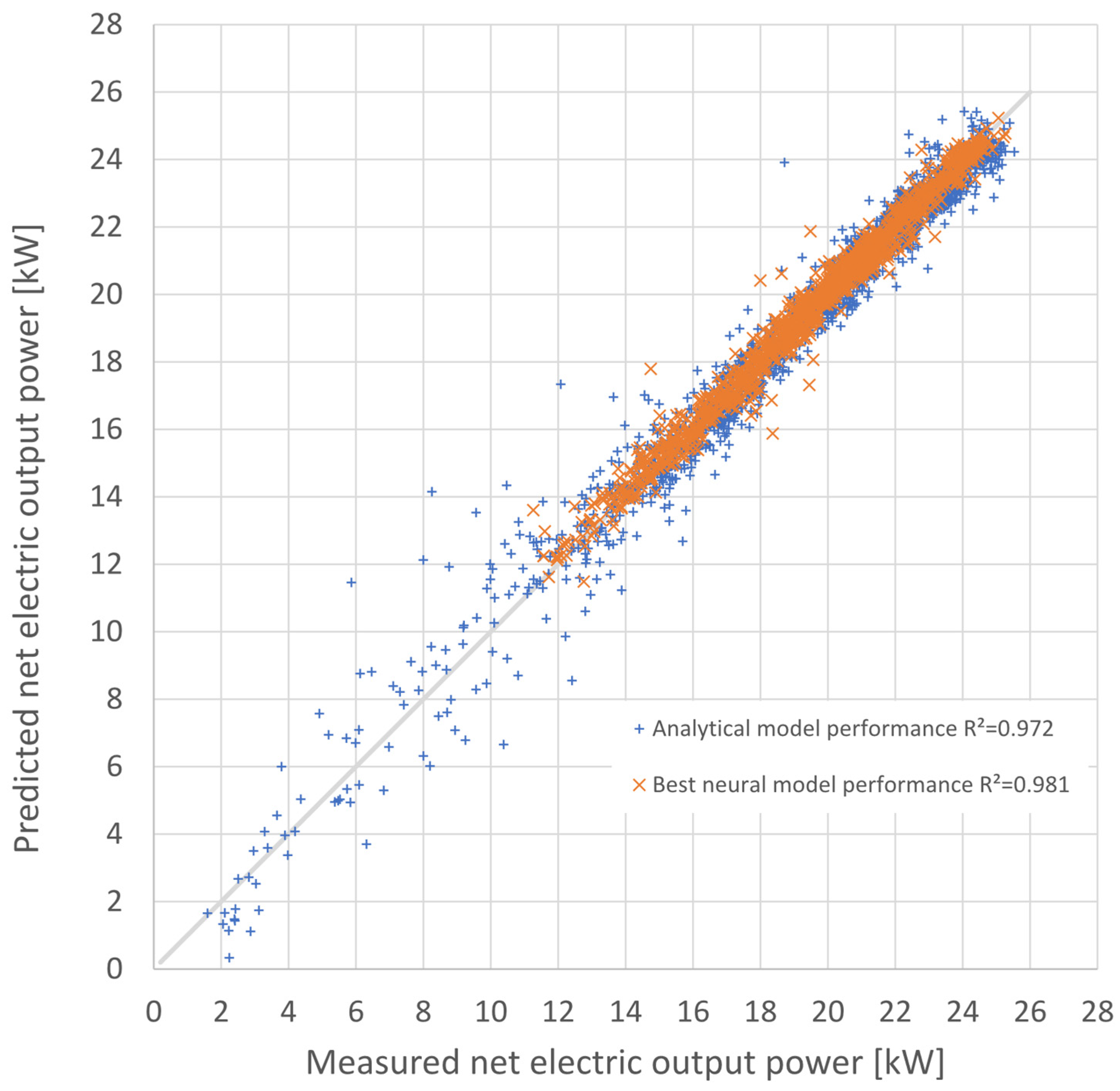
The study here presented aimed to test and optimise a forecasting model for the energy performance of a dish–Stirling solar-concentrating plant based upon the use of artificial neural networks. Contrary to most of the models already tested in the most recent literature in this scientific sector, the data used for the training phase of the networks were real data from a monitoring campaign of a real working plant on the university campus in Palermo. Neural networks of different architectures and sizes were also tested to better understand the link between the complexity and quality of the obtained results. All the different tested network architectures were trained alternately with two inputs (in the case of only standard data such as DNI and external temperature being available) and 12 inputs (in the case of more complete climatic data being available). A further reason for the novelty is the introduction of the input variables of information regarding the cleaning of the reflector mirrors, which has never before been tested in this type of model. The results made it possible to appreciate the good performance of the MLP models compared to the RBF models, traditionally characterised by better performance in the approximation of functions. Compared to a modern analytical model developed by the authors themselves, the best of the developed neural models obtained an even higher determination index between expected and calculated results, with a value equal to 0.98. The comparison is not, therefore, to be considered singularly, but it is useful to understand how a sophisticated neural network can be absolutely equivalent and sometimes superior to analytical models.

The results confirmed the maximum reliability of the developed ANN models.

It was not unexpected that the best neural model using the long input dataset, i.e., the one extended to twelve input variables, had a slightly higher accuracy than that achieved with the analytical energy model. The latter, being fundamentally based on a lumped parameter analysis of the dish–Stirling system, could not take into account the effect on its operation of all those meteorological and climatic variables that were, instead, considered in the extended dataset. For instance, it would be extremely complex to include the variability induced by air humidity or wind speed in the analytical model for predicting the electrical producibility of the solar concentrator, although these certainly influence the availability of direct solar radiation. The neural model, on the other hand, was based on a black-box approach, which simply learns from the available data without having to assume any analytical cause-and-effect relations between input and output. Thus, the present work demonstrates that the neural approach, using real data collected experimentally, is competitive with an analytical approach.

A neural model, already trained, together with the same input data used, is made available as attachments in “Supplementary Materials”. The digital neural model is directly provided with the script in Python language, allowing maximum transparency of the algorithms described in the research work. The availability of the dataset and the used Python scripts allow, thanks to the exclusive use of open-source software, maximum transparency and replicability. Finally, it should be noted that the results of the best of the neural networks tested (V-MLP-12) were better, in terms of coefficient of determination than one of the most advanced and highest performing analytical models developed by the same authors [18]. Further improvements in the performance of the neural network models could be achieved by using different activation functions and different optimisers (fine tuning) using the Python script and dataset provided as a complement to this study.

References

1. Graham, F. COP26: Glasgow Climate Pact signed into history. Nature 2021. Epub ahead of print. [Google Scholar] [CrossRef] [PubMed]
2. UNFCC. Glasgow Climate Change Conference – October-November 2021. Available online: https://unfccc.int/conference/glasgow-climate-change-conference-october-november-2021 (accessed on 1 November 2022).
3. IPCC. Global Warming of 1.5 °C. An IPCC Special Report on the impacts of global warming of 1.5 °C above pre-industrial levels and related global greenhouse gas emission pathways, in the context of strengthening the global response to the threat of clim. In Sustainable Development, and Efforts to Eradicate Poverty; Cambridge University Press: Cambridge, UK, 2018. [Google Scholar]
4. Pérez-Higueras, P.; Fernández, E.F. High Concentrator Photovoltaics: Fundamentals, Engineering and Power Plants; Springer: Berlin/Heidelberg, Germany, 2015. [Google Scholar]
5. Gielen, D.; Gorini, R.; Leme, R.; Prakash, G.; Wagner, N.; Janeiro, L.; Collins, S.; Kadir, M.; Asmelash, E.; Ferroukhi, R.; et al. World Energy Transitions Outlook: 1.5 °C Pathway; International Renewable Energy Agency: Masdar City, Abu Dhabi, 2021. [Google Scholar]
6. Elsheikh, A.H.; Panchal, H.; Ahmadein, M.; Mosleh, A.O.; Sadasivuni, K.K.; Alsaleh, N.A. Productivity forecasting of solar distiller integrated with evacuated tubes and external condenser using artificial intelligence model and moth-flame optimizer. Case Stud. Therm. Eng. 2021, 28, 101671. [Google Scholar] [CrossRef]
7. Moustafa, E.B.; Hammad, A.H.; Elsheikh, A.H. A new optimized artificial neural network model to predict thermal efficiency and water yield of tubular solar still. Case Stud. Therm. Eng. 2022, 30, 101750. [Google Scholar] [CrossRef]
8. Khan, J.; Arsalan, M.H. Solar power technologies for sustainable electricity generation—A review. Renew. Sustain. Energy Rev. 2016, 55, 414–425. [Google Scholar] [CrossRef]
9. Singh, U.R.; Kumar, A. Review on solar Stirling engine: Development and performance. Therm. Sci. Eng. Prog. 2018, 8, 244–256. [Google Scholar] [CrossRef]
10. Aqachmar, Z.; Ben Sassi, H.; Lahrech, K.; Barhdadi, A. Solar technologies for electricity production: An updated review. Int. J. Hydrogen Energy 2021, 46, 30790–30817. [Google Scholar] [CrossRef]
11. IRENA. Renewable Power Generation Costs in 2020; IRENA: Masdar City, Abu Dhabi, 2020. [Google Scholar]
12. IEA. Concentrated Solar Power (CSP), IEA, Paris. 2021. Available online: https://www.iea.org/reports/concentrated-solar-power-csp (accessed on 11 October 2022). License: CC BY 4.0..
13. International Energy Agency (IEA). Global Energy Review: CO2 Emissions in 2020; IEA: Paris, France, 2020. [Google Scholar]
14. Lovegrove, K.; Stein, W. Concentrating Solar Power Technology: Principles, Developments and Applications; Woodhead Publushing: Cambridge, UK, 2012; ISBN 9781845697693. [Google Scholar]
15. Fuqiang, W.; Ziming, C.; Jianyu, T.; Yuan, Y.; Yong, S.; Linhua, L. Progress in concentrated solar power technology with parabolic trough collector system: A comprehensive review. Renew. Sustain. Energy Rev. 2017, 79, 1314–1328. [Google Scholar] [CrossRef]
16. Schiel, W.; Keck, T. 9—Parabolic dish concentrating solar power (CSP) systems. In Concentrating Solar Power Technology; Lovegrove, K., Stein, W., Eds.; Woodhead Publishing Series in Energy; Woodhead Publishing: Cambridge, UK, 2012; pp. 284–322. ISBN 978-1-84569-769-3. [Google Scholar]
17. Salameh, Z. Chapter 5—Emerging Renewable Energy Sources. In Renewable Energy System Design; Salameh, Z., Ed.; Academic Press: Boston, MA, USA, 2014; pp. 299–371. ISBN 978-0-12-374991-8. [Google Scholar]
18. Buscemi, A.; Lo Brano, V.; Chiaruzzi, C.; Ciulla, G.; Kalogeri, C. A validated energy model of a solar dish-Stirling system considering the cleanliness of mirrors. Appl. Energy 2020, 260, 114378. [Google Scholar] [CrossRef] [Green Version]
19. Schiel, W.; Schweiber, A.; Stine, W.B. Evaluation of the 9-kw e dish/stirling system of schlaich bergermann und partner using the proposed iea dish/stirling performance analysis guidelines. In Proceedings of the Intersociety Energy Conversion Engineering Conference, Monterey, CA, USA, 7–12 August 1994. [Google Scholar]
20. Yang, S.; Wan, M.P.; Chen, W.; Ng, B.F.; Dubey, S. Model predictive control with adaptive machine-learning-based model for building energy efficiency and comfort optimization. Appl. Energy 2020, 271, 115147. [Google Scholar] [CrossRef]
21. Korkmaz, D. SolarNet: A hybrid reliable model based on convolutional neural network and variational mode decomposition for hourly photovoltaic power forecasting. Appl. Energy 2021, 300, 117410. [Google Scholar] [CrossRef]
22. Chen, Z.; Yu, H.; Luo, L.; Wu, L.; Zheng, Q.; Wu, Z.; Cheng, S.; Lin, P. Rapid and accurate modeling of PV modules based on extreme learning machine and large datasets of IV curves. Appl. Energy 2021, 292, 116929. [Google Scholar] [CrossRef]
23. Elsheikh, A.H.; Sharshir, S.W.; Abd Elaziz, M.; Kabeel, A.E.; Guilan, W.; Haiou, Z. Modeling of solar energy systems using artificial neural network: A comprehensive review. Sol. Energy 2019, 180, 622–639. [Google Scholar] [CrossRef]
24. Khosravi, A.; Syri, S.; Pabon, J.J.G.; Sandoval, O.R.; Caetano, B.C.; Barrientos, M.H. Energy modeling of a solar dish/Stirling by artificial intelligence approach. Energy Convers. Manag. 2019, 199, 112021. [Google Scholar] [CrossRef]
25. Khoshaim, A.B.; Moustafa, E.B.; Bafakeeh, O.T.; Elsheikh, A.H. An optimized multilayer perceptrons model using grey wolf optimizer to predict mechanical and microstructural properties of friction stir processed aluminum alloy reinforced by nanoparticles. Coatings 2021, 11, 1476. [Google Scholar] [CrossRef]
26. Elsheikh, A.H.; Abd Elaziz, M.; Ramesh, B.; Egiza, M.; Al-qaness, M.A.A. Modeling of drilling process of GFRP composite using a hybrid random vector functional link network/parasitism-predation algorithm. J. Mater. Res. Technol. 2021, 14, 298–311. [Google Scholar] [CrossRef]
27. Zaaoumi, A.; Bah, A.; Ciocan, M.; Sebastian, P.; Balan, M.C.; Mechaqrane, A.; Alaoui, M. Estimation of the energy production of a parabolic trough solar thermal power plant using analytical and artificial neural networks models. Renew. Energy 2021, 170, 620–638. [Google Scholar] [CrossRef]
28. Ahmadi, M.H.; Sorouri Ghare Aghaj, S.; Nazeri, A. Prediction of power in solar stirling heat engine by using neural network based on hybrid genetic algorithm and particle swarm optimization. Neural Comput. Appl. 2013, 22, 1141–1150. [Google Scholar] [CrossRef]
29. Liao, T.; Lin, J. Optimum performance characteristics of a solar-driven Stirling heat engine system. Energy Convers. Manag. 2015, 97, 20–25. [Google Scholar] [CrossRef]
30. Beltrán-Chacon, R.; Leal-Chavez, D.; Sauceda, D.; Pellegrini-Cervantes, M.; Borunda, M. Design and analysis of a dead volume control for a solar Stirling engine with induction generator. Energy 2015, 93, 2593–2603. [Google Scholar] [CrossRef]
31. Vahidi Bidhendi, M.; Abbassi, Y. Exploring dynamic operation of a solar dish-stirling engine: Validation and implementation of a novel TRNSYS type. Sustain. Energy Technol. Assess. 2020, 40, 100765. [Google Scholar] [CrossRef]
32. Zayed, M.E.; Zhao, J.; Elsheikh, A.H.; Zhao, Z.; Zhong, S.; Kabeel, A.E. Comprehensive parametric analysis, design and performance assessment of a solar dish/Stirling system. Process Saf. Environ. Prot. 2021, 146, 276–291. [Google Scholar] [CrossRef]
33. Zayed, M.E.; Zhao, J.; Li, W.; Elsheikh, A.H.; Abd Elaziz, M.; Yousri, D.; Zhong, S.; Mingxi, Z. Predicting the performance of solar dish Stirling power plant using a hybrid random vector functional link/chimp optimization model. Sol. Energy 2021, 222, 1–17. [Google Scholar] [CrossRef]
34. Backes, J.G.; D’Amico, A.; Pauliks, N.; Guarino, S.; Traverso, M.; Lo Brano, V. Life Cycle Sustainability Assessment of a dish-Stirling Concentrating Solar Power Plant in the Mediterranean area. Sustain. Energy Technol. Assess. 2021, 47, 101444. [Google Scholar] [CrossRef]
35. Lemmon, E.W.; Bell, I.H.; Huber, M.L.; McLinden, M.O. NIST Standard Reference Database 23: Reference Fluid Thermodynamic and Transport Properties-REFPROP, Version 10.0, National Institute of Standards and Technology. Stand. Ref. Data Program Gaithersbg. 2018. [Google Scholar]
36. Gil, R.; Monné, C.; Bernal, N.; Muñoz, M.; Moreno, F. Thermal Model of a Dish Stirling Cavity-Receiver. Energies 2015, 8, 1042–1057. [Google Scholar] [CrossRef] [Green Version]
37. Molugaram, K.; Rao, G.S. Random Variables. Stat. Tech. Transp. Eng. 2017, 113–279. [Google Scholar] [CrossRef]
38. Samanes, J.; Garcia-Barberena, J. A model for the transient performance simulation of solar cavity receivers. Sol. Energy 2014, 110, 789–806. [Google Scholar] [CrossRef]
39. Guarino, S.; Buscemi, A.; Ciulla, G.; Bonomolo, M.; Lo Brano, V. A dish-stirling solar concentrator coupled to a seasonal thermal energy storage system in the southern mediterranean basin: A cogenerative layout hypothesis. Energy Convers. Manag. 2020, 222, 113228. [Google Scholar] [CrossRef]
40. Ahmadi, M.H. Investigation of Solar Collector Design Parameters Effect onto Solar Stirling Engine Efficiency. J. Appl. Mech. Eng. 2012, 1, 10–13. [Google Scholar] [CrossRef] [Green Version]
41. Buscemi, A.; Guarino, S.; Ciulla, G.; Lo Brano, V. A methodology for optimisation of solar dish-Stirling systems size, based on the local frequency distribution of direct normal irradiance. Appl. Energy 2021, 303, 117681. [Google Scholar] [CrossRef]
42. Gulli, A.; Kapoor, A.; Pal, S. Deep Learning with TensorFlow 2 and Keras: Regression, ConvNets, GANs, RNNs, NLP, and More with TensorFlow 2 and the Keras API; Packt Publishing Ltd.: Birmingham, UK, 2019. [Google Scholar]
43. Singh, P.; Manure, A. Learn TensorFlow 2.0: Implement Machine Learning and Deep Learning Models with Python; Springer: Berlin/Heidelberg, Germany, 2020. [Google Scholar]
44. Brownlee, J. Deep Learning with Python: Develop Deep Learning Models on Theano and TensorFlow Using Keras; Machine Learning Mastery: San Juan, PR, USA, 2016. [Google Scholar]
45. Brownlee, J. Machine learning mastery with python. Mach. Learn. Mastery Pty Ltd. 2016, 527, 100–120. [Google Scholar]
46. Moolayil, J.; Moolayil, J.; John, S. Learn Keras for Deep Neural Networks; Springer: Berlin/Heidelberg, Germany, 2019. [Google Scholar]
47. Tian, Z.; Zhang, Y.; Liu, K.; Zhao, J. Topic Knowledge Acquisition and Utilization for Machine Reading Comprehension in Social Media Domain. In Proceedings of the China National Conference on Chinese Computational Linguistics, Hohhot, China, 13–15 August 2021; pp. 161–176. [Google Scholar]
48. Principe, J.C.; Euliano, N.R.; Lefebvre, W.C. Neural and Adaptive Systems: Fundamentals through Simulations; Wiley: Hoboken, NJ, USA, 1999; ISBN 978-0-471-35167-2. [Google Scholar]
49. Jiang, Q.; Zhu, L.; Shu, C.; Sekar, V. An efficient multilayer RBF neural network and its application to regression problems. Neural Comput. Appl. 2021. [Google Scholar] [CrossRef]
50. He, X.; Xu, S. Process Neural Networks: Theory and Applications; Springer Science\Business Media: Berlin/Heidelberg, Germany, 2010. [Google Scholar]
51. Bilogur, A. Radial Basis Networks and Custom Keras Layers. Available online: https://www.kaggle.com/residentmario/radial-basis-networks-and-custom-keras-layers (accessed on 1 November 2022).
Figure 1. The dish–Stirling concentrator plant that is installed at the University of Palermo.
Energies 15 09298 g001
Figure 2. Dynamic viscosity for hydrogen, helium, and air versus temperature with a pressure value of 20 MPa.
Energies 15 09298 g002
Figure 3. The location of the reference dish–Stirling system (Palermo, Italy).
Energies 15 09298 g003
Figure 4. Statistical analysis of some variables included in the original dataset.
Energies 15 09298 g004
Figure 5. Correlation matrix of variables of the original dataset without outliers (Pearson correlation coefficient).
Energies 15 09298 g005
Figure 6. The layout of the dish–Stirling concentrator plant.
Energies 15 09298 g006
Figure 7. Flow chart of the overall energy model.
Energies 15 09298 g007
Figure 8. General architectures of (a) multilayer perceptron and (b) radial basis function neural networks.
Energies 15 09298 g008
Figure 9. Histogram of residuals showing the probability density distribution of residuals resulting from the validation process of V-MLP-2.
Energies 15 09298 g009
Figure 10. A Q–Q (quantile–quantile) plot resulting from the validation process of V-MLP-2.
Energies 15 09298 g010
Figure 11. A predicted versus measured power output (W) resulting from the validation process of V-MLP-2.
Energies 15 09298 g011
Figure 12. Histogram of residuals showing the probability density distribution of residuals resulting from the validation process of V-MLP-12.
Energies 15 09298 g012
Figure 13. A Q–Q (quantile–quantile) plot resulting from the validation process of V-MLP-12.
Energies 15 09298 g013
Figure 14. A predicted versus measured graph resulting from the validation process of V-MLP-12.
Energies 15 09298 g014
Figure 15. Performance comparison between an analytical and the best neural network model, V-MLP-12 [18].
Energies 15 09298 g015