Review

A Comparative Analysis of Maximum Power Point Techniques for Solar Photovoltaic Systems

by
Ashwin Kumar Devarakonda
1,
Natarajan Karuppiah
1,
Tamilselvi Selvaraj
2,
Praveen Kumar Balachandran
1,*,
Ravivarman Shanmugasundaram
1 and
Tomonobu Senjyu
3,*
1
Department of EEE, Vardhaman College of Engineering, Hyderabad 501218, Telangana, India
2
Department of EEE, Sri Sivasubramaniya Nadar College of Engineering, Chennai 603110, Tamil Nadu, India
3
Faculty of Engineering, University of the Ryukyus, Okinawa 903-0213, Japan
*
Authors to whom correspondence should be addressed.
Energies 2022, 15(22), 8776; https://doi.org/10.3390/en15228776
Submission received: 19 October 2022 / Revised: 18 November 2022 / Accepted: 18 November 2022 / Published: 21 November 2022
(This article belongs to the Section K: State-of-the-Art Energy Related Technologies)

Abstract

:
The characteristics of a PV (photovoltaic) module is non-linear and vary with nature. The tracking of maximum power point (MPP) at various atmospheric conditions is essential for the reliable operation of solar-integrated power generation units. This paper compares the most widely used maximum power point tracking (MPPT) techniques such as the perturb and observe method (P&O), incremental conductance method (INC), fuzzy logic controller method (FLC), neural network (NN) model, and adaptive neuro-fuzzy inference system method (ANFIS) with the modern approach of the hybrid method (neural network + P&O) for PV systems. The hybrid method combines the strength of the neural network and P&O in a single framework. The PV system is composed of a PV panel, converter, MPPT unit, and load modelled using MATLAB/Simulink. These methods differ in their characteristics such as convergence speed, ease of implementation, sensors used, cost, and range of efficiencies. Based on all these, performances are evaluated. In this analysis, the drawbacks of the methods are studied, and wastage of the panel’s available output energy is observed. The hybrid technique concedes a spontaneous recovery during dynamic changes in environmental conditions. The simulation results illustrate the improvements obtained by the hybrid method in comparison to other techniques.

1. Introduction

Daily energy demand is rising and normally, to meet those demands, energy is produced by using non-renewable sources such as coal, natural gas, etc., [1,2]. This creates a high amount of carbon emissions. As many countries have decided to pair with zero carbon emission nations, the use of renewable energy sources is increasing day by day [3,4]. Due to the free abundance of solar energy, solar panel utilization is increasing rapidly. However, the efficiency of the solar panel is 13–19% [5]. The reasons for these low efficiencies are rapidly changing atmospheric conditions and the circuits attached to them such as loads, charge controllers, and other devices [6,7,8].
Our main aim is to choose a controller which should be able to track MPP properly, by which we can use the solar panel up to its maximum capacity. During its operation, a solar panel sees the load as varying. Therefore, it delivers a lower amount of power during its operation and MPP is lost [9,10,11,12]. For maintaining the MPP operation of the panel, the amount of resistance seen across the PV panel should be fixed such that the solar panel sees a fixed load, i.e., the resistance seen across the panel is fixed (Ro is fixed) and the solar panel produces the maximum amount of power [13,14]. The MPPT techniques monitor the output voltage and output current of the solar panels and give a particular operating point to the panel such that the maximum amount of power is delivered.
Many algorithms are developed but traditional methods such as P&O and incremental conductance are widely used because of their simplicity; however, the energy losses are higher with these methods [15]. Computational power and development of microcontrollers have given rise to methods such as fuzzy logic, particle swarm, neural network, ANFIS, hybrid models, ant bee colony, …, etc.
The various conventional MPPT techniques such as fractional open circuit voltage (FOCV) [16], fractional short circuit current (FSCC) [17], curve fitting (CF) [17], hill climbing (HC) [18], incremental conductance (INC) [19], etc. can be observed from the references. The main drawbacks of FOCV and FSCC are less accurate, as they are mostly used for low-power applications [16,17]. Popular techniques such as P&O, INC and HC work well, but only produce maximum power during constant insolation conditions, so they are not effective under variable irradiations and shading conditions [18,19]. These methods also suffer from poor convergence, more amount of steady-state oscillations, and the slow tracking of MPP [20].
For better steady-state performance, transient behaviour Intelligent MPPT methods such as neural network, fuzzy logic, and ANFIS are used [21,22,23]. To overcome difficulties caused by the PI controller, fuzzy controllers have been proposed, as they provide high-performance control, but they lead to a high amount of computational burden and their usage is limited in complex systems [24].
In the method of P&O with multi-layer ANN, the training of the model and the collection of the datasets is a challenging task [25], and the ANFIS technique consolidates the power of fuzzy logic and neural networks but the training process requires more numerical calculations for accurate results, which is tough; if the models are not properly trained, the inaccurate response of the hybrid models contain a greater number of oscillations [26].
A neural network is a fast solution for enhancing efficiency, and it has the ability to deal with uncertainties and can handle the problem without any prior knowledge [27]. In NN, MPP is tracked in a faster way by modifying the weights of layers according to the learning algorithm. NN controllers show good performance under rapidly varying irradiance and partial shading, in terms of efficiency and responses [10,28].
Apart from conventional methods, intelligent methods provide a better performance, and the artificial intelligence overcomes drawbacks caused by methods such as Genetic Algorithms (GA) [29], Pattern Swarm Optimization (PSO) [30], fuzzy logic (FL) [31], Grey Wolf Optimization (GWO) [32], etc. However, the complexity of design and implementation matters.
The category of hybrid methods reflects the combination of two or more methods of the above-mentioned methods, and the combination increases the effectiveness of the models. Hybrid models such as P&O with multi-layer ANN [33], ANN with a variable step size of P&O [34], Genetic Algorithms, P&O with incremental conductance [34], Gravitational search algorithm with particle swam optimization, and many other algorithms have been proposed but each of them has complexity levels based on their applications. The effective application of algorithm tracking of the maximum power point and the solar panel efficiency can be improved [35].
Modern algorithms vary in their effectiveness, complexity of circuits, and convergence speed. For good results, traditional methods can be combined with alternative methods to track MPP under varying conditions [36,37,38]. The ease of implementation of P&O, and the accuracy and rapid recovery of the neural network cannot be ignored, so the combination of these methods helps to reduce uncertainties in the output response. This paper compares a hybrid control that removes the uncertainties which are seen in P&O, INC, and other algorithms. With the use of the hybrid controller [39], the performance of solar panels is improved, and the combination present in the model removes the inaccurate responses and it gives a reliable performance in varying atmospheric conditions as well [40,41].
The efficiencies of algorithms are calculated based on the energy generated in the time interval. Based on the references, MPPT techniques were implemented. In the study, a standalone PV system with a boost converter and dc load is considered.
However, choosing MPPT for specific PV system designs and situations might be confusing, since each approach has its own set of benefits and drawbacks. There is a noticeable rise in new approaches for hybrid, optimization techniques, so analysis is essential to study new methodologies. This paper provides an MPPT comparison based on the tracking of MPP under constant and varying conditions. This paper provides an evaluation based on efficiency, tracking accuracy, and complexity. Furthermore, this comparison paper may be a useful resource for researchers.

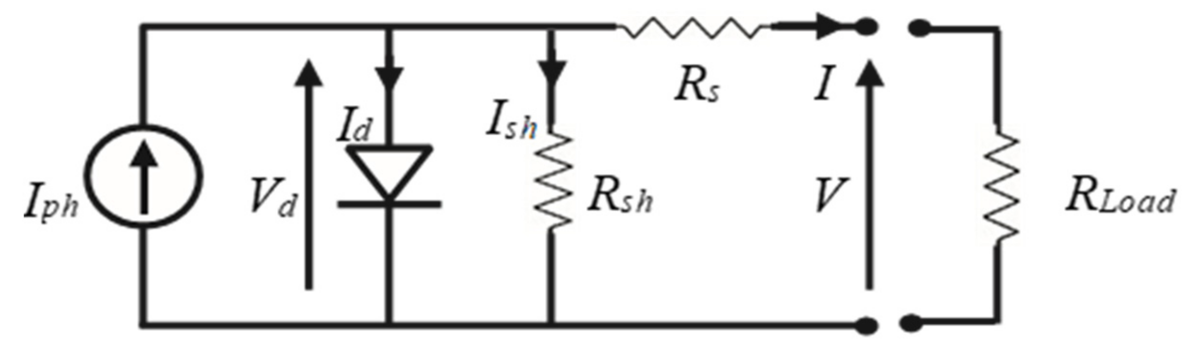
2. Modelling of a Photovoltaic Cell

A PV cell consists of a P-N semiconductor junction when it is exposed to light; it generates its equivalent electrical output. PV arrays comprise a series of/parallel combinations of solar cells. The electrical equivalent of a solar cell is shown in Figure 1. It is represented by a light-generated current source with a shunt diode D, along with parallel and series resistance.
The Shockley diode equation is used to calculate the characteristic electrical equation of a PV cell. It is written as
I = I ph I sat × [ exp q × V + R S × I nKT 1 ] V + R S × I R sh
where I = solar cell current, Iph = generated photocurrent, Isat = reverse saturation diode current, q = charge of electron = 1.60217 × 10⁻¹⁹ C, k = Boltzmann constant = 1.3807 × 10⁻²³ J/k, n = diode’s ideality factor, T = cell temperature, Rs = series resistance, Rsh = shunt resistance.
The current Iph generated is directly proportionate to sun radiation, and the arrangement of series and parallel resistance shows the voltage losses when connected to external contacts and leakage current. Figure 2 and Figure 3 depict the module’s p-v curve for different values of irradiation and temperature.
The simulation model of the PV block has been used for obtaining the curves, and for more power, cells are connected in a series of/ parallel combinations to build a PV array.
The output characteristics of the panel are nonlinear and depend on temperature and irradiation. To obtain maximum power from the panel, the resistance seen by the panel should be maintained constant. For this purpose, a power converter such as a DC-DC boost converter is utilized for load matching to the PV panel, to obtain the maximum power out of the panel.

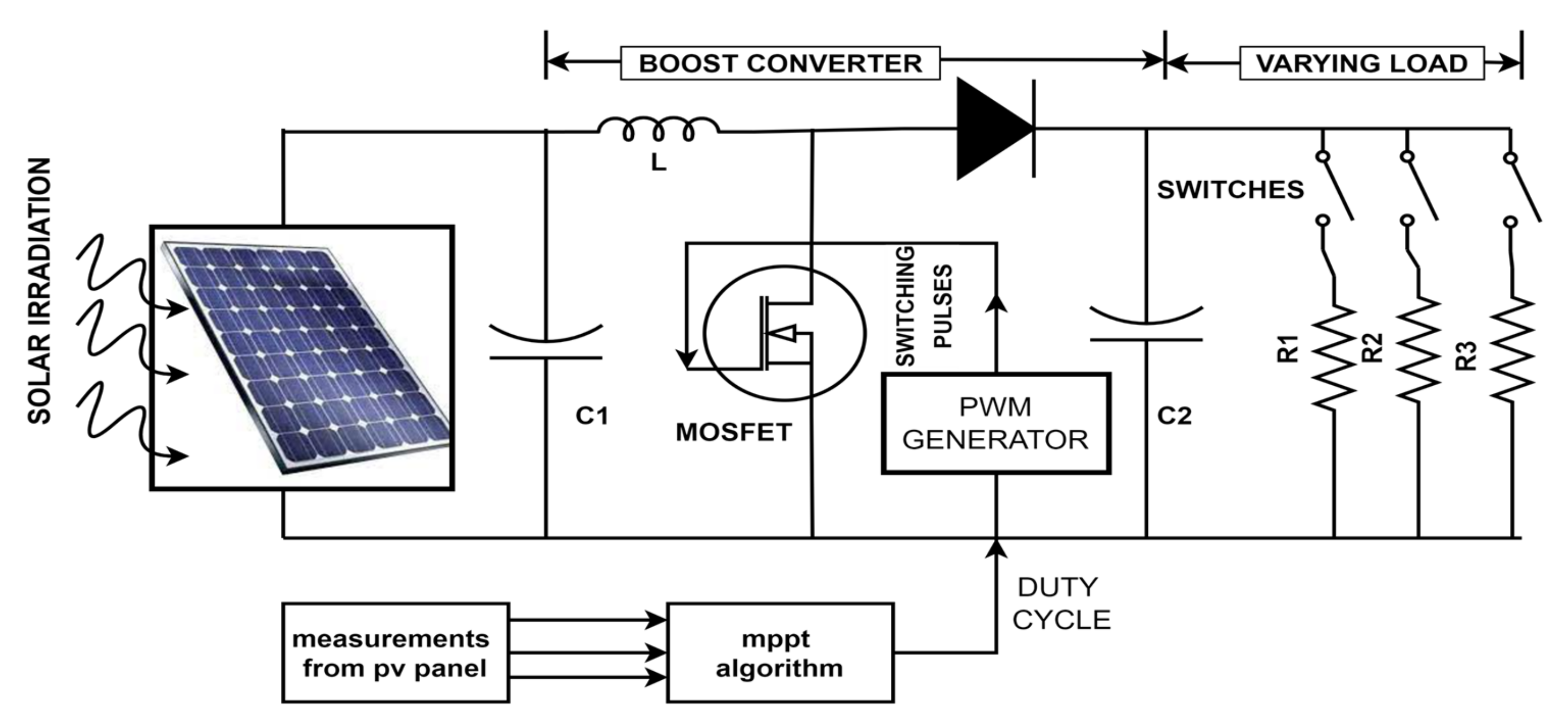
3. DC-DC Boost Converter

A boost converter serves as a switch mode regulator, converting an unregulated dc output voltage to a controlled dc output voltage. A boost converter (Figure 4) comprises a switch K (transistor/MOSFET), diode, filter capacitor, an inductor, as well as a resistor.
The control operation is performed by controlling the switch’s duty ratio, and in continuous mode, when the switch is ON, the diode is in an OFF state and energy is stored in the inductor. When the switch is OFF, the stored energy is dissipated in the resistor, through the diode path.
The output voltage of the converter is given as
V o = V i   ( d 1 d )  
where d = duty cycle.

4. MPPT Control

In a PV module, there is one single operating point at a given point of time where maximum power can be drawn. The operation mainly depends on the load characteristics to which it is connected. If a panel is directly connected to a load, the operating point of the panel is not optimal. Therefore, an MPPT controller should be connected between them.
The MPPT controller adjusts the resistance seen by the panel RT, such that it sees a constant load, so as the output changes, the control input to the converter changes such that the input impedance of the controller is maintained as constant.
In such a case, RT seen from PV will remain constant, irrespective of load resistance. From this, the operating point will be maintained constant and the maximum power will be drawn from the panel. The MPPT control scheme for the solar panel is shown in Figure 5, and the specifications can be found in Table 1.

4.1. MPPT Algorithms

Many techniques have been developed for implementing MPPT. The techniques differ in implementation, cost, speed, and efficiency. The most widely used are perturb & observe method (P&O), incremental conductance (INC), and fuzzy logic control method.

4.2. Perturb and Observe Method

Owing to its simple design and ease of operation and execution, the perturbation and observation technique is the most widely used technique. The concept behind the P&O method is to modify the operating voltage of the solar cell until the maximum power is obtained from it. The impact on the system is observed by modifying the system voltage.
If the operating point lies in regions 1, and 2 in Figure 6 [11], the perturbation is adjusted such that the point reaches the MPP. If the operating voltage is perturbed and if the power is increased (dp/dv > 0), then we can see that point is now moving towards the MPP, whereas if it decreases (dp/dv < 0), then the direction of perturbation is reversed. The process will continue until the MPP is reached at every point in time. Based on the previous duty ratio, the next duty ratio is calculated by checking the differences between the power and voltage values.
The flow chart of the P&O algorithm is shown in Figure 7.
The P&O algorithm could not track the MPP under rapidly varying atmospheric changes. The system has been tested for various levels of irradiation, load, and temperatures (shown in Table 2).
The performance of the system for various levels of perturbation size is seen in Figure 8. It indicates that with an increasing/decreasing Dprev value, the rise time taken to obtain the MPP does not become affected, but by increasing the Dprev value, the smoothness of the curve increases.
The performance of the system for constant and varying atmospheric conditions is shown in Figure 9, Figure 10, Figure 11 and Figure 12. The output reaches a maximum at 0.05 s (Figure 9), and then the output is maintained constant at 247 W. At variable irradiation and variable loads in Figure 10, we can observe that the output waveform takes time to get back to the steady state after disturbances and output power changes with respect to the input. Only under varying loads, the output is nearly constant except at load disturbances (Figure 11). At variable temperatures and variable loads, the output wave took time to reach the steady point. However, after load disturbance, it reached the steady point quickly under input variations (Figure 12).

4.3. Incremental Conductance Method

The incremental conductance method employs the current and the voltage as measuring units to detect the output current and voltage of the solar array. Here, both parameters are sensed simultaneously [2,3]. In this method, the value of incremental conductance is seen in the graph (Figure 13) [6]. We can see that slope (dp/dv) of the curve at the MPP of the PV panel is zero on the left side (+ve) and the right side (−ve).
The relationship between the voltage and the current is given as
dp   dv = d vi dv = I + V dI dV
From the above equation, the relationship in the curve is given as
di dv = i v   at   mpp  
di dv > i v   left   of   mpp
di dv < i v   right   of   mpp
The MPP can be traced by relating the above conditions, i.e., instantaneous conductance and incremental conductance. The direction of the perturbation is determined by the conditions. The system oscillates around the MPP and the controls the amplitude of oscillations. It decreases as the increases.
As   di dv + i v
However, the operating point moves away from the MPP, so the should be chosen carefully. As a result, the error caused by changes in irradiance is eliminated; however, the cost and complexity of the system increase. The main difference between P&O and INC is the direction of the perturbation.
The algorithm performance for various atmospheric conditions is shown in Figure 14, Figure 15, Figure 16 and Figure 17, Varying load, constant temperature and irradiation are seen in Figure 16, except at load disturbances, where the output is almost constant. In Figure 17, constant irradiation, load, temperature, and output is maintained constant at 250 W. In variable irradiation and loads, as seen in Figure 16, we can observe that under load and input variations, the output has quickly gained a steady point without a time lag. Under variable temperatures and loads, as seen in Figure 17, we can observe that initially the output reached nearly 290 W and the output almost followed the temperature variations and was nearly maintained at 230 to 250 W, except at load disturbances.

4.4. Fuzzy Logic Controller Method

Fuzzy—“not clear, distinct, precise, blurred”. Fuzzy logic control (FLC) is operated as a mathematical system that addresses uncertainty and deals with input data that is imprecise, ambiguous, noisy, or missing [3].
With the development of computational power, the fuzzy logic method has become more popular. In fuzzy logic, an analog input signal is compared to a present logical variable membership function or fuzzy logic rules with values between zero and one. Because of its heuristic nature, simplicity, as well as effectiveness in both non-linear and linear systems, this method has been widely used. Because of its numerous advantages, the FL method is among the most effective techniques for obtaining MPP in solar systems. It is resistant to imprecise inputs, does not need a precise mathematical system, and is relatively easy to design. It offers a mathematical framework for transforming linguistic control rules expressed as (IF-THEN) statements through an automatic control strategy. The input variables of (FLC) are defect value (E), change of defect value (ΔE), and one output value, which alters the duty ratio ΔD (as seen in Figure 18). The intake values E and ΔE at any point of time, k, are indicated as
E k = P K P k 1 V k V k 1 = dp dv
Δ E k = E k E k 1
P(k) is the solar cell’s output power and V(k) is the output voltage at the “k” moment.
E(k) indicates the load operating point position, i.e., on the left/right of MPP.
The fuzzy logic system consists of a fuzzification block, an inference engine block, and a defuzzification block.
The process of execution of the fuzzy logic control method can be observed in Figure 19.

4.4.1. Fuzzification

This block converts the crisp value to a fuzzy value by using knowledge and databases and uses membership functions to define the input variables into fuzzy variables. The membership functions for the parameters E(k), CE(k), as well as the output parameters dD(k), in which each membership function of five fuzzy rule sets, PS (Positive Small), PB (Positive Big), NS (Negative Small), NB (Negative Big), and ZE (Zero Equivalent) can be seen in Figure 20, Table 3.
A larger number of linguistic terms improve the accuracy of output stability. It does, however, increase the algorithm’s complexity, and the computing time.

4.4.2. Fuzzy Inference System (FIS)

FIS consists of a fuzzy rule base which takes fuzzy variables as inputs and generates possible fuzzy outputs, given as input to the defuzzifier (if-then), etc. It is the main part of the fuzzy system; with this, inputs are mapped to an output. In this model, we have used the Mamdani inference system.
Based on the inputs, FLC determines its next setpoint based on the parameters of the Fuzzy logic rule framework, which operates on a set of conditional rules. It is determined by the designer’s professional experience as well as the operation of the control system. This paper employs 25 fuzzy control rules, which are presented in Table 3. Those conditions are defined as (Conditional statements (IF-THEN)) with the following syntax: IF (E is Negative Big) and (ΔE is Zero Equivalent) THEN (ΔD is Positive Big).
Case 1: If the term (E) is +ve, the position is mainly found to the leftward of the MPP. If the term (CE) is +ve, the action point shifts closer to the MPP. If the term CE is −ve, the opposite happens.
Case 2: If the term E is −ve, the position is located to the rightward of the MPP. If the term CE is −ve, the action point drifts farther from the MPP, and the opposite happens if CE is −ve.
The procedure is implemented as a sequence of fuzzy IF-THEN rules.

4.4.3. Defuzzification

FLC generates a fuzzy subset as its output. Defuzzification is needed as real-world systems require precise control values. This block converts the fuzzy variable into crisp values using various defuzzification methods such as the center of gravity, weighted average, and mean of maximum. It creates a mapping from the fuzzy logic system to the concerned implied output into a non-fuzzy control signal.
The controller performance for various atmospheric conditions is shown in Figure 21, Figure 22, Figure 23 and Figure 24. The fuzzy logic method nearly took 0.05 s to reach the maximum point; it quickly regained the steady point under load variations, as can be seen in Figure 21. From Figure 22, we can observe that except for initial lag, the output was maintained constant at 248 W. Under variable irradiations and loads, the output power disturbance lag mainly observed at first disturbance was only 0.3 s, and at remaining points, the effect was overcome quickly in Figure 23. For temperature and load variations in Figure 24, we observe that initially, the output was above 250 W, and disturbances can be clearly observed in the output wave. Except for the disturbances, we can notice that the output has almost remained between 210 W to 250 W.

4.5. Neural Network Method

Neural networks (NN) are a form of artificial intelligence method that teaches a computer to process data in a manner similar to the human mind. The artificial intelligence technique performs better than traditional approaches [7]. The demerits of traditional methods include delayed responses to quick variations in solar irradiance and temperatures, as well as failure to track the maximum output power point.
Solar temperature and irradiance temperature are used as inputs to the neural network. The number of layers is determined by the hit-and-trial method. The duty ratio for the converter is the output. To begin working with any NN algorithm, training points must be collected. The training data is obtained by varying temperature and insolation values for the PV array and collecting duty ratios for finding maximum power. Some test points are fixed while training to check their performance post-training. “NNTOOL” is used to train a neural network in MATLAB. A set of 1000 data points are captured to train the neural network. Specifically, the temperature range is (15 to 35 degrees) and the irradiance range is from (0 to 1000 W/m2).
The neural network tool kit used in neural network training can be seen in Figure 25a, and the performance of the neural network can be analyzed by mean square error(MSE) versus the epoch graph(Figure 25b). We obtain the best performance at the 1000 epoch, which is 2.3045 × 10⁻¹¹; the training state validations and the error histograms can be observed in (Figure 25c,d), and by the regression plot in Figure 25e, we observe the relationship between the dependent and independent variables, and we observe that the data and fit are aligned, which shows only the smallest possible error. From Figure 25f, we see the training, validation, and testing results of the trained data of 1000 points—indicating a very small error. The step-by-step executions of a neural network can be seen in Figure 26.
  • Solar panel data used for training the neural network and ANFIS
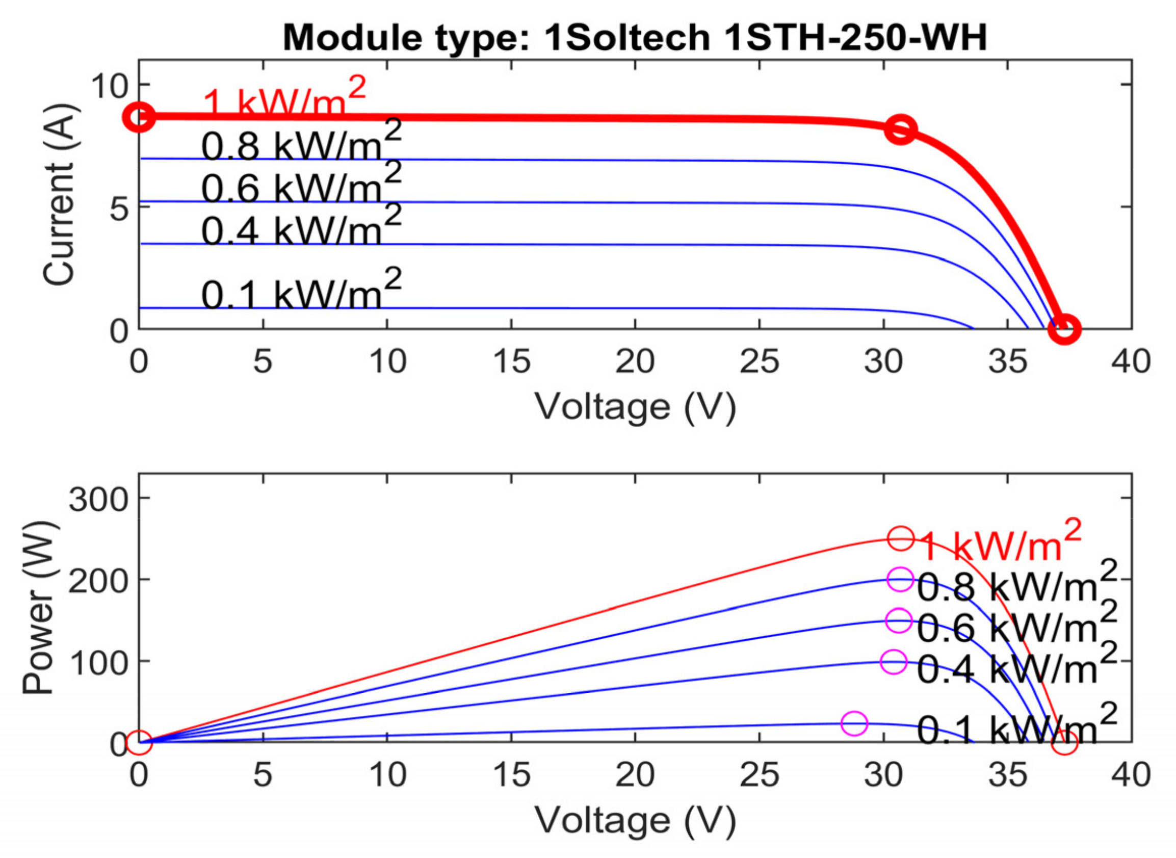
  • Short circuit current = 8.66 A;
  • Maximum power point current = 8.15 A;
  • Open-source voltage = 37.3 V;
  • Maximum power point voltage = 30.7;
  • Alpha = 0.086998;
  • Beta = −0.36901;
In the fitting problem, a neural network to map between the data set of numeric inputs and a set of numeric targets is decided. The requirements used for training the neural network are listed in Table 4.
The controller’s performance can be observed in Figure 27, Figure 28, Figure 29 and Figure 30. At variable loads and constant irradiation and temperature, in Figure 27 we observe that it took nearly 0.05 s to track the maximum point, and gaining the steady point is also quick, except at the points where the output is constant. In Figure 28, we can observe the output is maintained constant at 240 W. In Figure 29, we can observe that the output gained a steady point quickly, except at the 0.3 s disturbance, where the remaining curves were smooth for the remaining disturbances. In Figure 30, we can observe that up to 0.4 s the output was not tracked properly, as it was below 150 W, and after 0.4 s, the output was close to 240 W up to 0.8 s, and after 0.8 s, the output is 210 W, except at load disturbances.

4.6. ANFIS Method (Adaptive Neuro-Fuzzy Inference System)

In ANFIS and fuzzy systems, the same numbers of nodes are present; they are fuzzifications of input variables (layer-1) and logic-based rules and fuzzy inference systems (layers 2 and 3), defuzzification (layer-4), and aggregation (layer-5). The ANFIS architecture (in Figure 31) employs NN architecture with five determined layers [9]. The ANFIS structure for a given model of discrete-time data with n inputs values is y t i , y t j , , y t l   and one output w i and is based on first order (SUGENO) rule-base with “m”-rules [12].
If   y t k   is   x k j   then   y t j   =   θ j 0   +   k = i l θ j k y t k θ j k
where y t k is x kj as assumption portion and
y t j   =   θ j 0   +   k = i l θ j k y t k
as subsequent segments; θ jk , θ j 0 as linear parameters; x kj as nonlinear parameters; j = 1 , 2 , , m ; k = i , j , , l , and if w 1 , w 2 , , w i are the firing strengths for m values y t 1 , y t 2 , , y t m , then the calculated output w i can be given as:
y i = w ¯ 1 y t i + w ¯ 2 y t j + + w ¯ m y t l

Adaptive Neuro-Fuzzy Controller

The MPPT control structure by incorporating ANFIS can be designed to achieve the MPP by modifying the duty ratio based on the changes of E(k) and CE (k). ANFIS trains an FL model with two inputs and one output to detect a logical rule; the execution process of ANFIS can be seen in Figure 32. The general structure of the ANFIS rule is given as:
  • Rule i: if E(k) is Xi1 and CE(k) is Xi2, then
(Duty)i = yi1 × 1 + yi2 × 2
where
  • (Duty)i is the changing duty cycle and
  • Xij is the membership function.
Figure 32. Flow chart of ANFIS technique.
Energies 15 08776 g032
The performance of the algorithm for various atmospheric conditions can be seen in Figure 33, Figure 34, Figure 35 and Figure 36. From Figure 33, we observe that an initial lag was present in the tracking output, and later, except for load disturbances, the output was constant. In Figure 34, we can see that the output was constantly maintained close to 250 W. In Figure 35, we observe that except for the disturbance at 0.3 s, the output wave has a smooth gain up to the steady point. In Figure 36, we can see that after 0.05 s, the output was nearly 275 W and the output was maintained close to 245 W, except for load disturbances up to 0.8 s, at which point, after0.8 s, the output was reduced to 160 W.

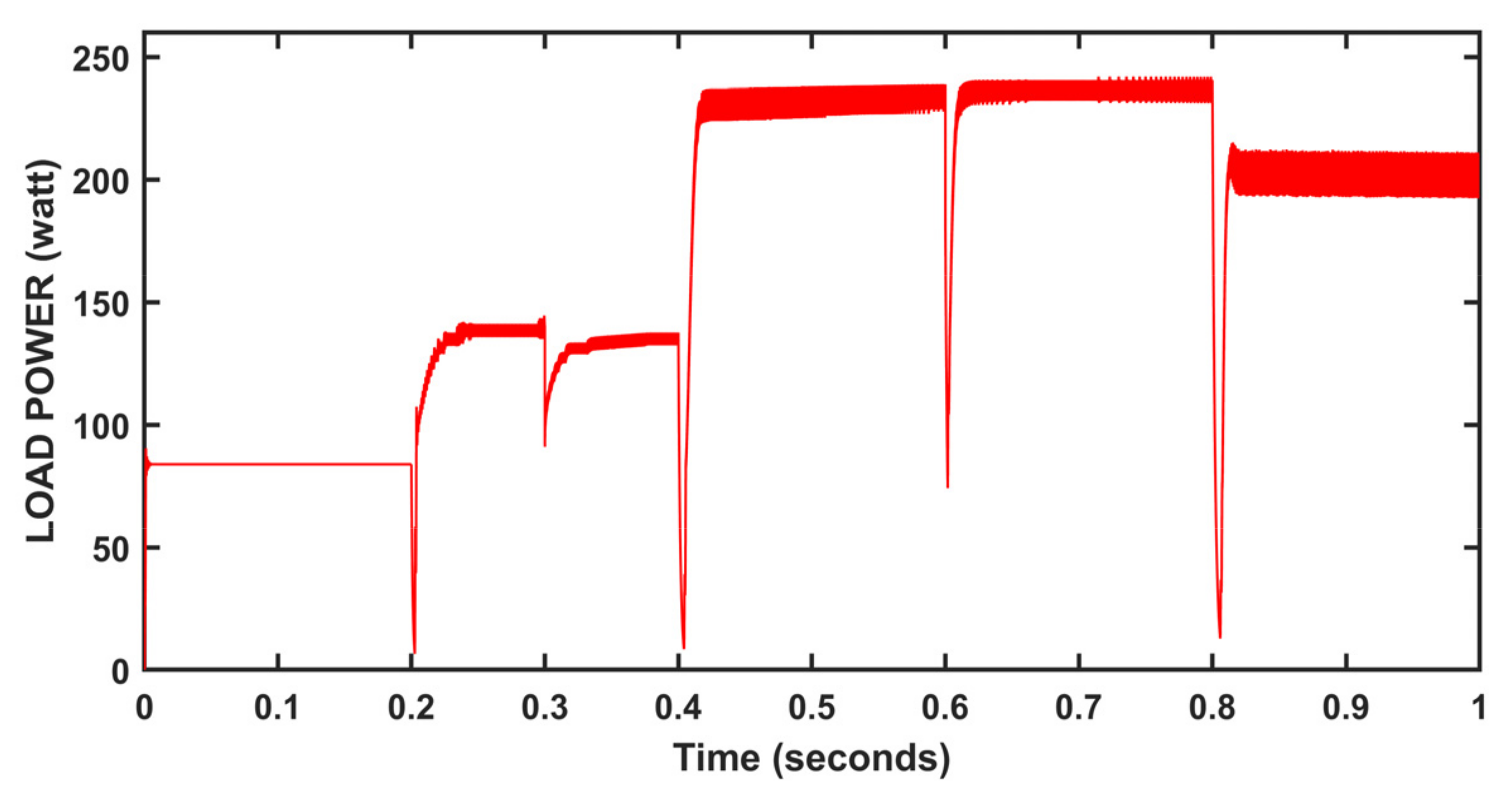
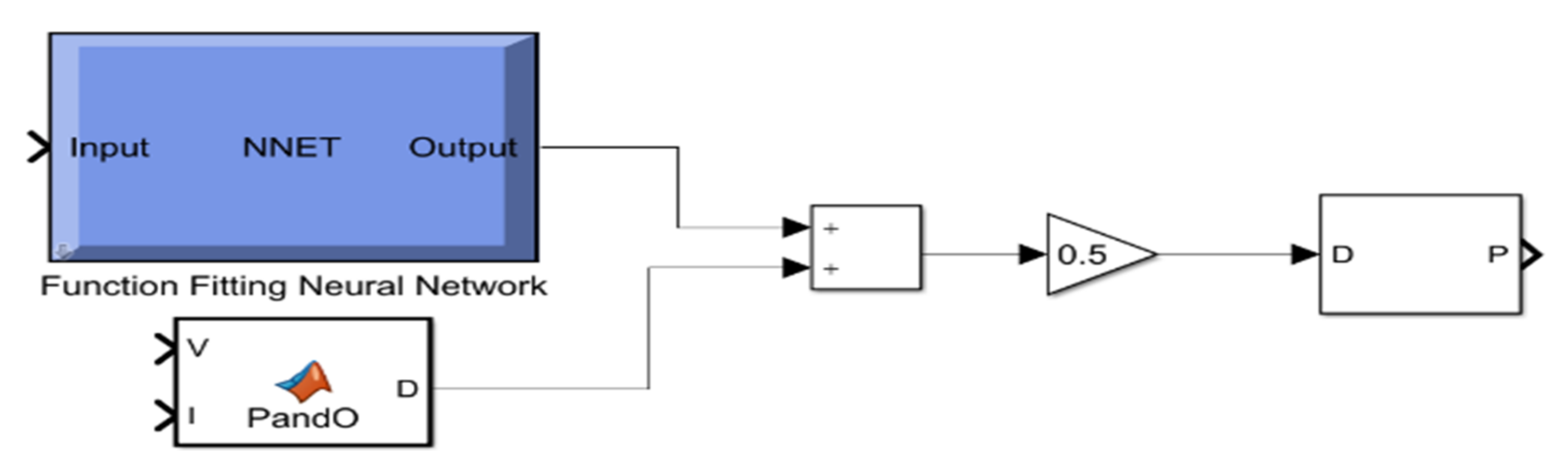
4.7. Hybrid Method (Neural Network and P&O)

For maintaining maximum power and increasing efficiency during varying environmental conditions, the hybrid technique is based on a combination of two controllers, the NN and P&O methods. In the neural network, the input layer has two nodes, the hidden layer has eight nodes, and the output layer has one node. The main scheme of the hybrid algorithm is using the NN controller to yield a prediction of the voltage value during varying insolation levels, such that a change in irradiation is very small. If the change is not small, the step size in the P&O method will be too low to reach the MPP, which results in oscillations [22].
The above figure shows the modern hybrid model control for MPPT. In this algorithm, the inputs are the current, the voltage of the PV panel, and the variation of power. The maximum power can be obtained by the neural network learning algorithm, the changing weights of neurons, and combining the results with the P&O algorithm result. In this control method, the neural network output is combined with the output and the average of the duty ratio generated is given to the PWM generator for generating switching pulses (Figure 37). The error in the duty ratio is reduced when both the methods’ duty ratios are added, resulting in a reduced error duty cycle; because of these techniques, the oscillations around the maximum power point are reduced [17], and the process of execution can be seen in Figure 38.
Based on the observation of powers at various points by the P&O method and the neural network method, the maximum powers are set for converter operation. Furthermore, maximum power is adjusted according to environmental conditions; this method helps in reducing the cost of the system by reducing the number of sensors, compared to other complex-hybrid methods for tracking MPP with good efficiency. The hybrid methods vary in terms of speed of action, measuring speculations, hardware execution, number of sensors, and unpredictability.
D1 = duty cycle generated by P&O
D2 = duty cycle generated by the Neural network
D = (D1 + D2)/2
The performance of the controller for various atmospheric conditions can be observed in Figure 39, Figure 40, Figure 41 and Figure 42. From Figure 39, we can observe that it tracked MPP quickly and also under the disturbances, the deviations were also fewer. In Figure 40, we can see that output was maintained as nearly constant between 240 to 250 W. In Figure 41, we can observe that the initial output was nearly 250 W, except for the disturbance at 0.3 s, where the output was in a steady state until the next variation. The output gained quickly from variations and no time lag was observed, and the curve was smooth for the remaining variations. In Figure 42, we can observe that for up to 0.4 s, the output was not tracked properly and after 0.4 s the output was maintained at 245 W, except for the disturbance at 0.6 s up to 0.8 s, at which point after 0.8 s the output is maintained at 210 W.

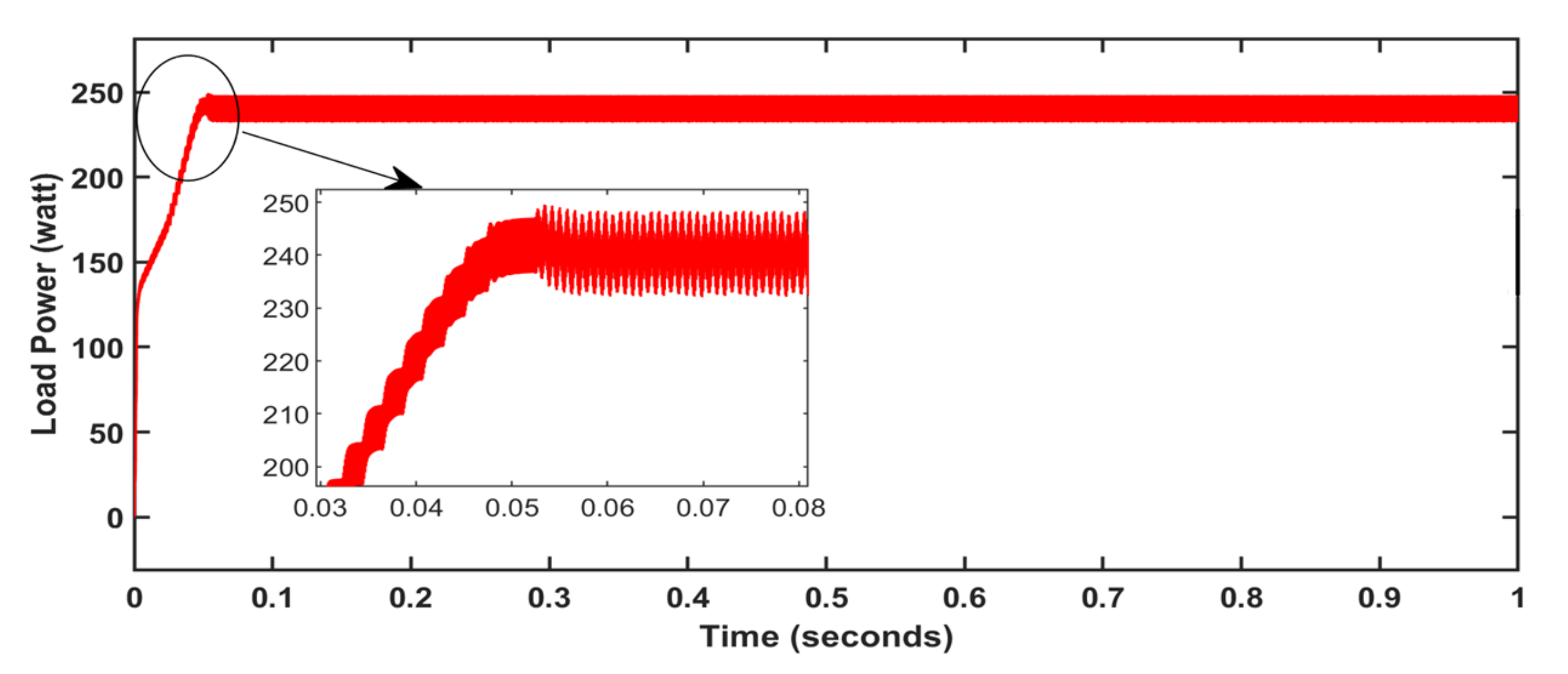
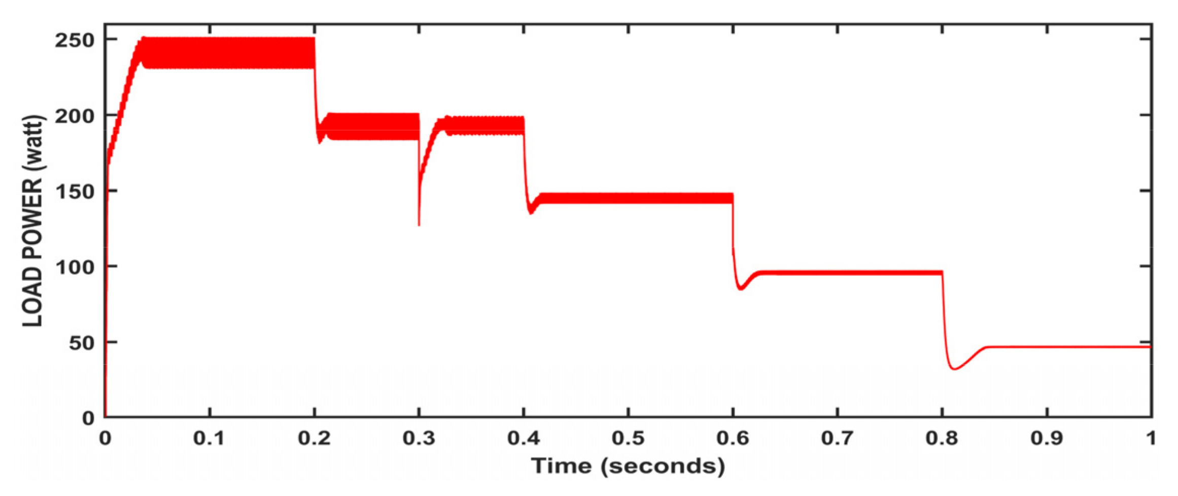
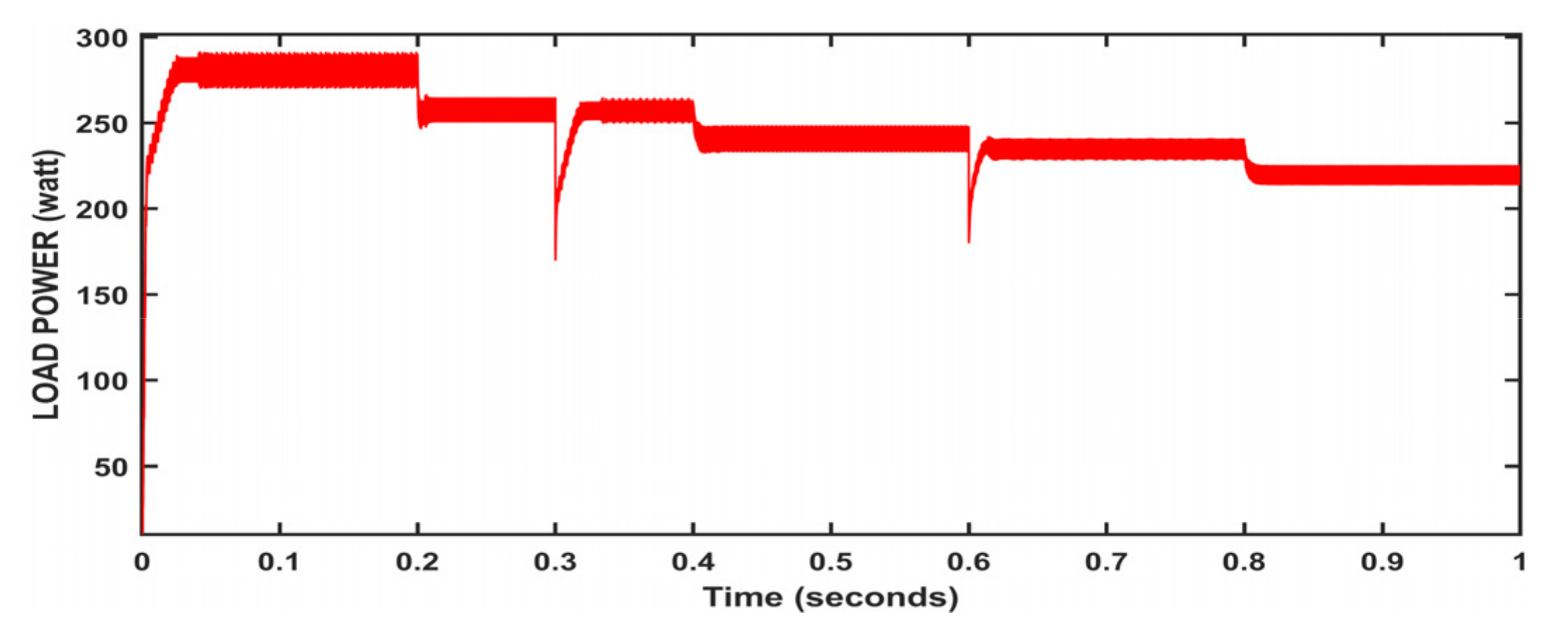
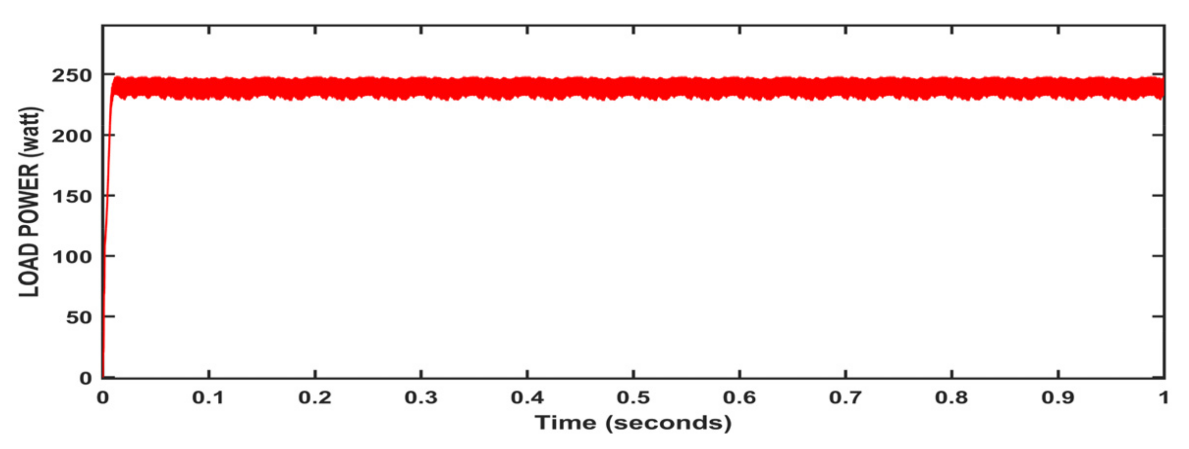
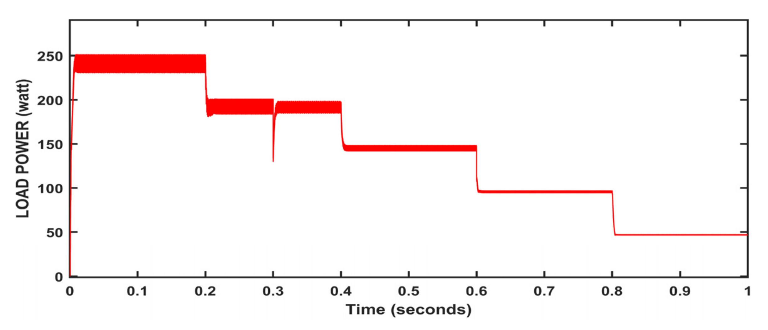
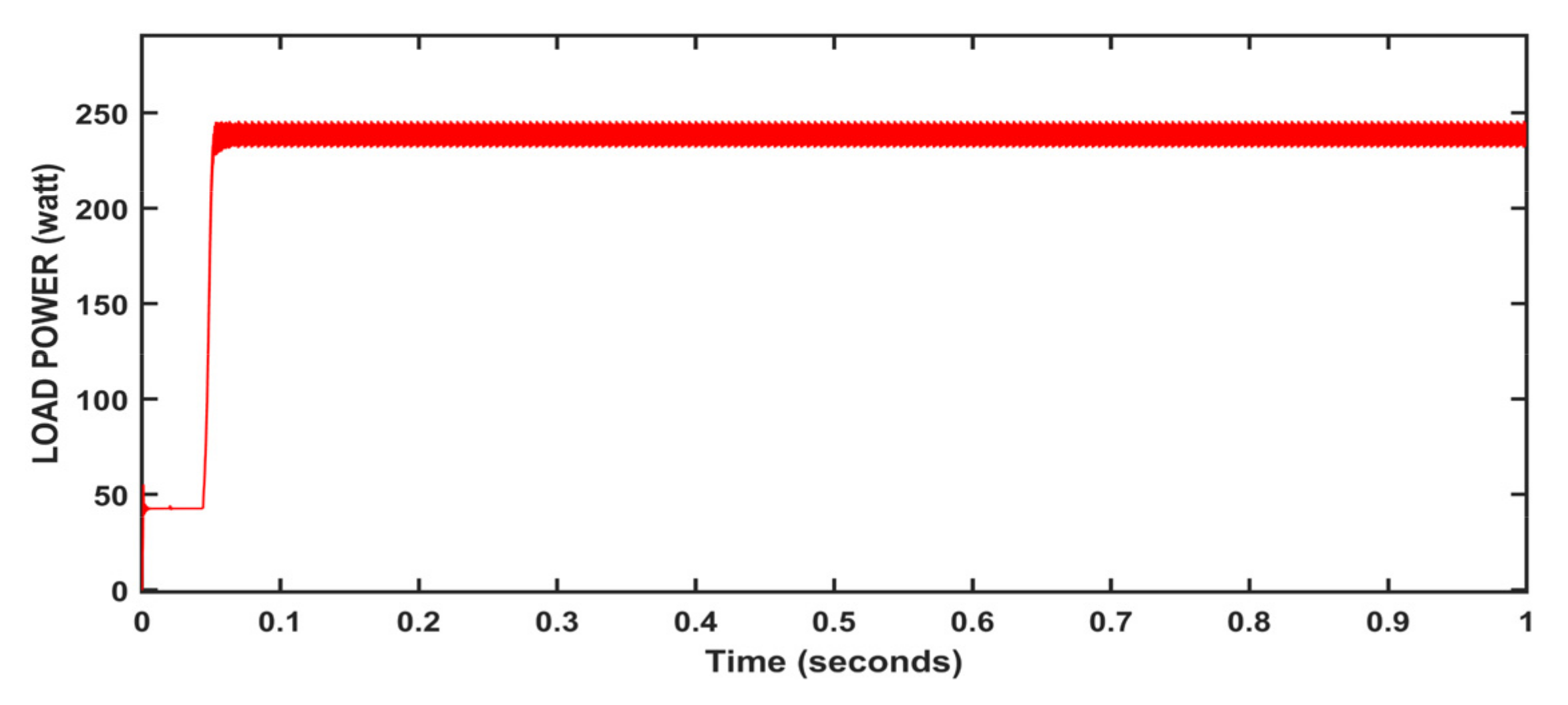
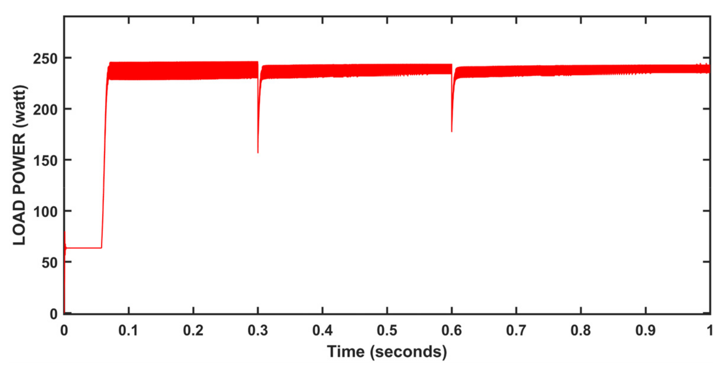
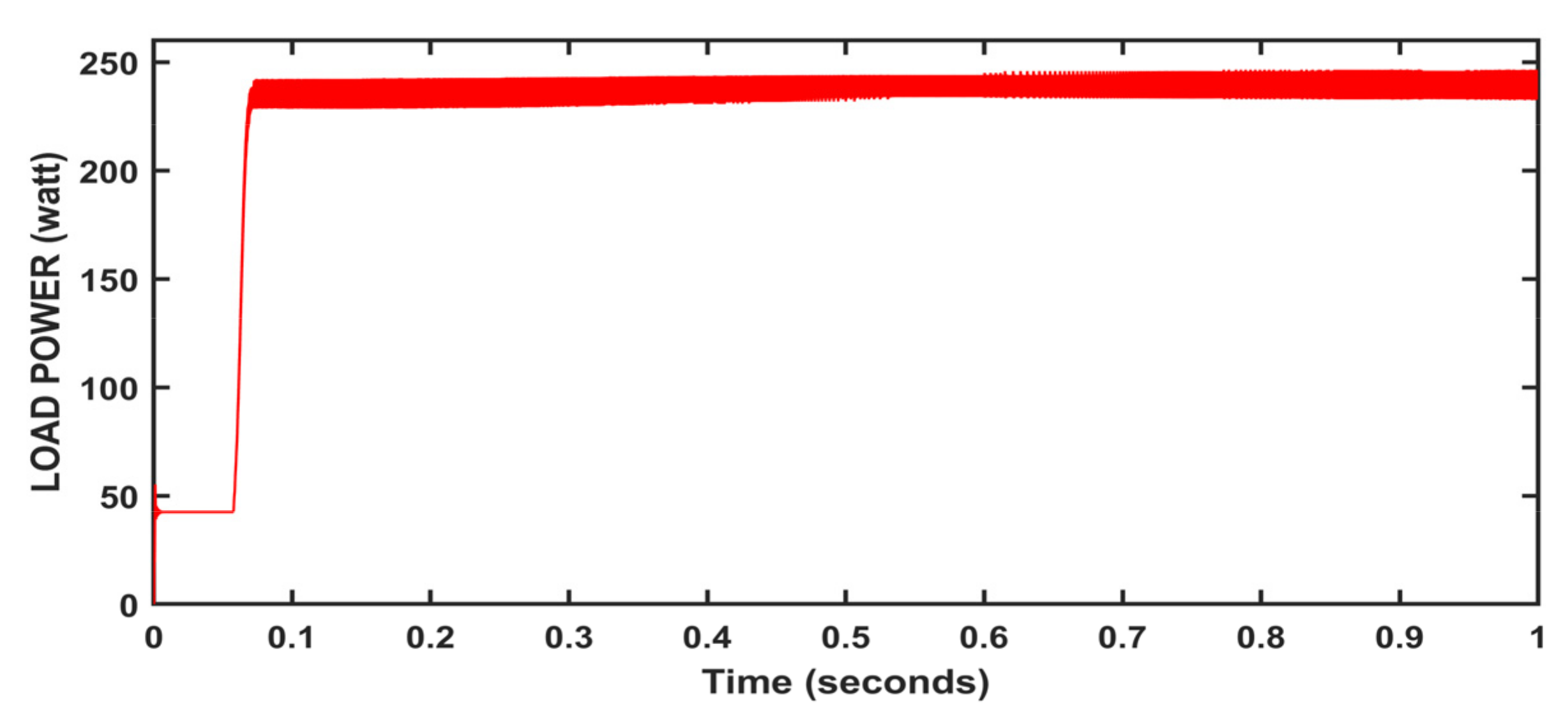
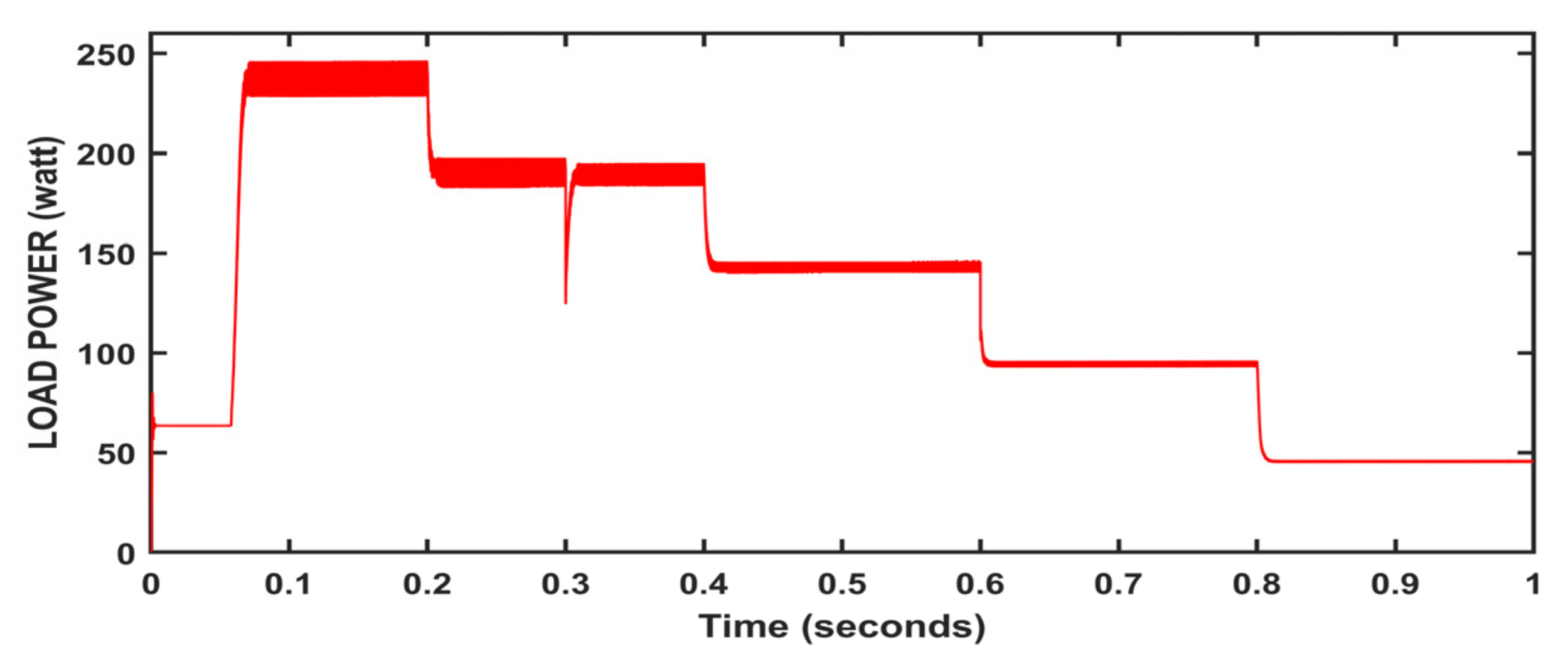
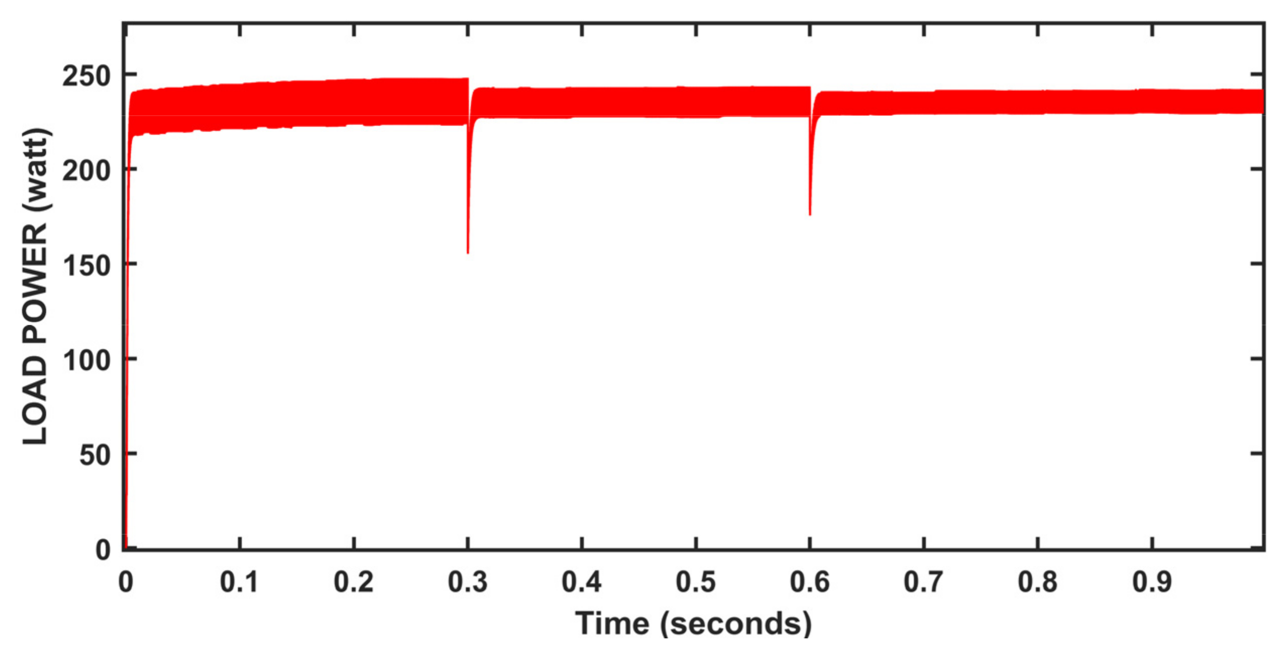
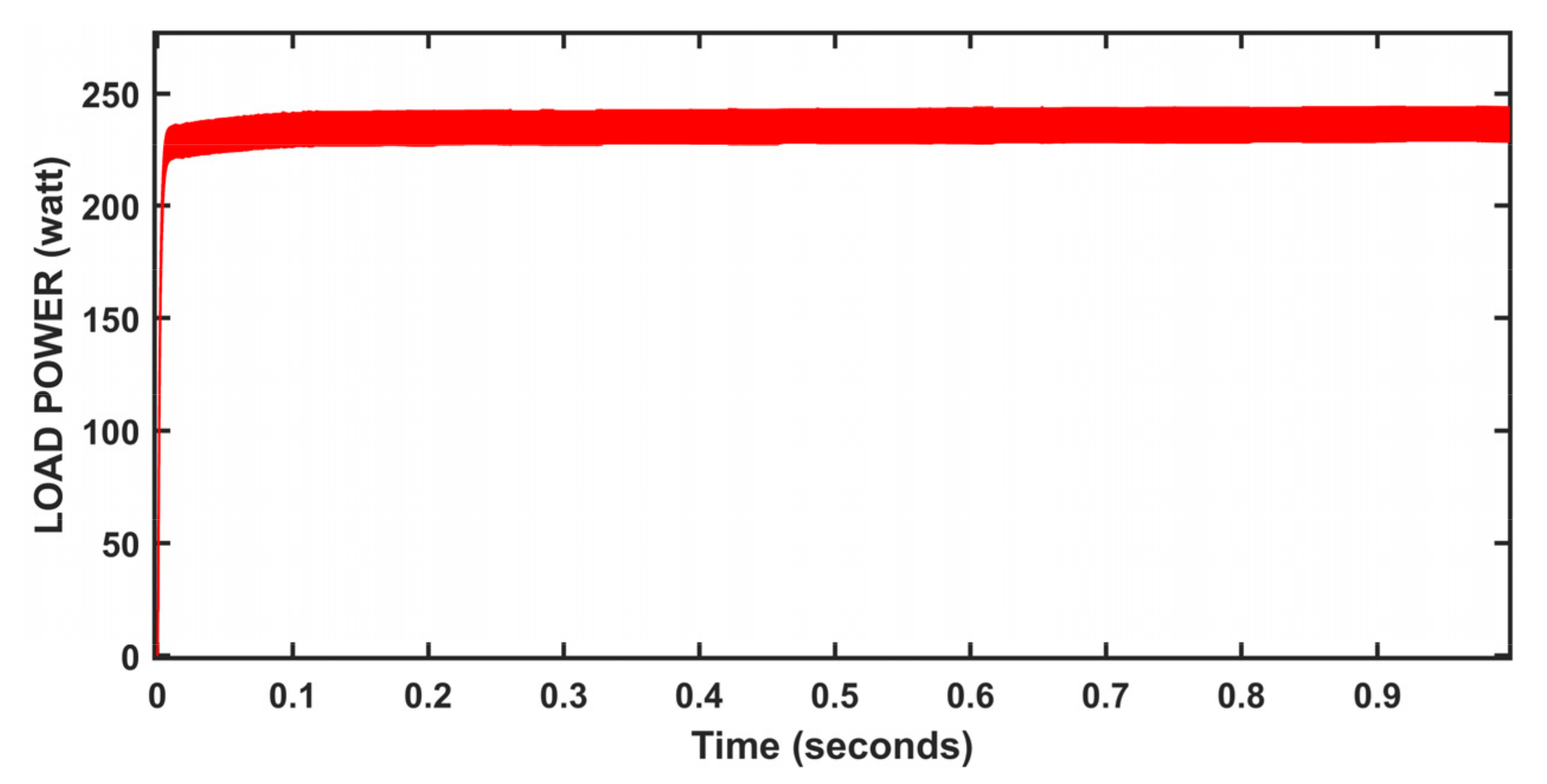
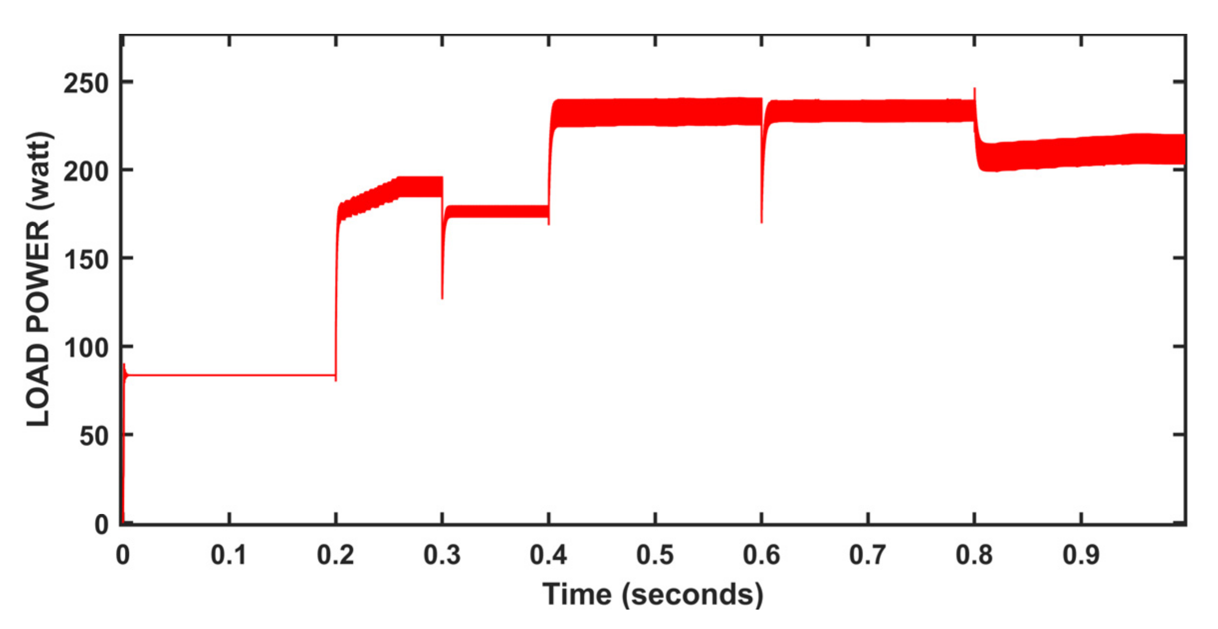
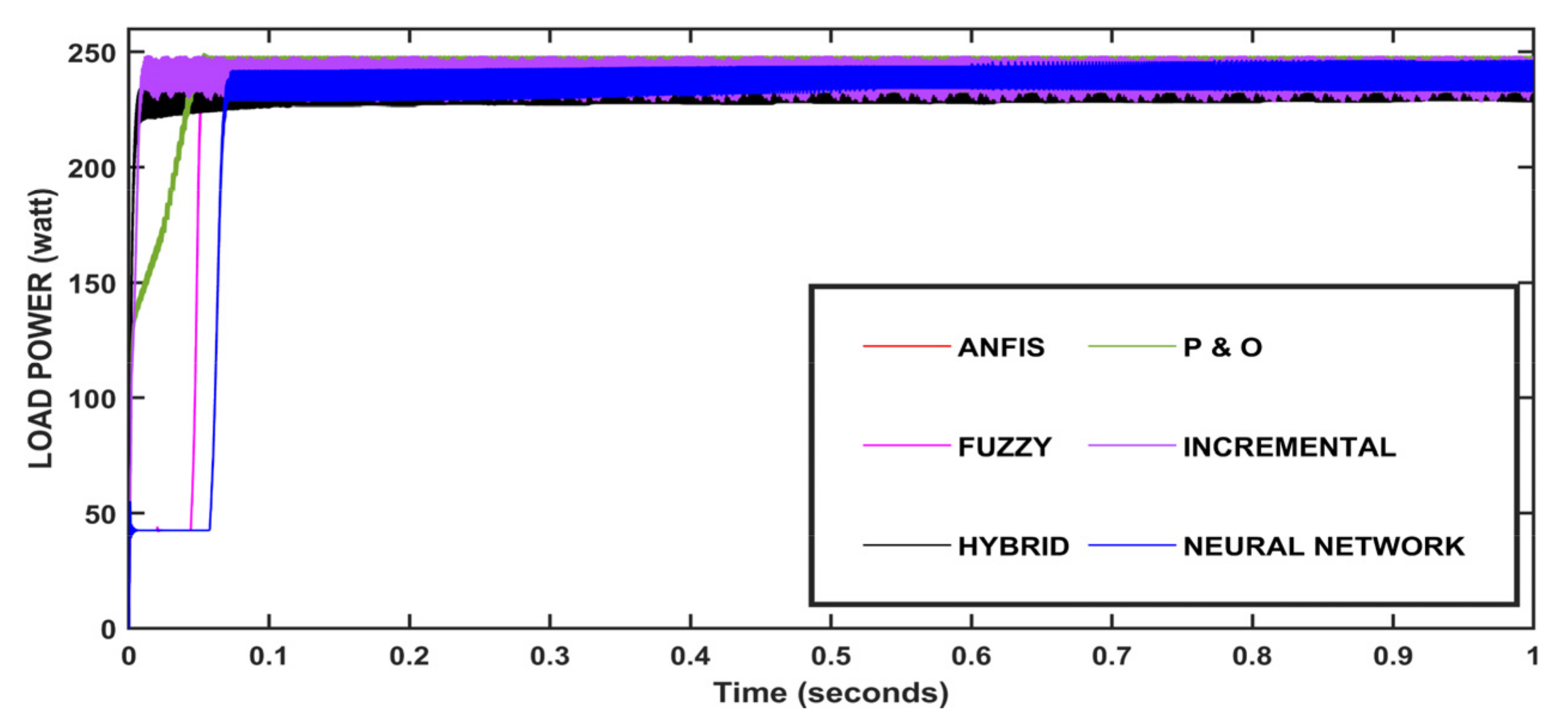
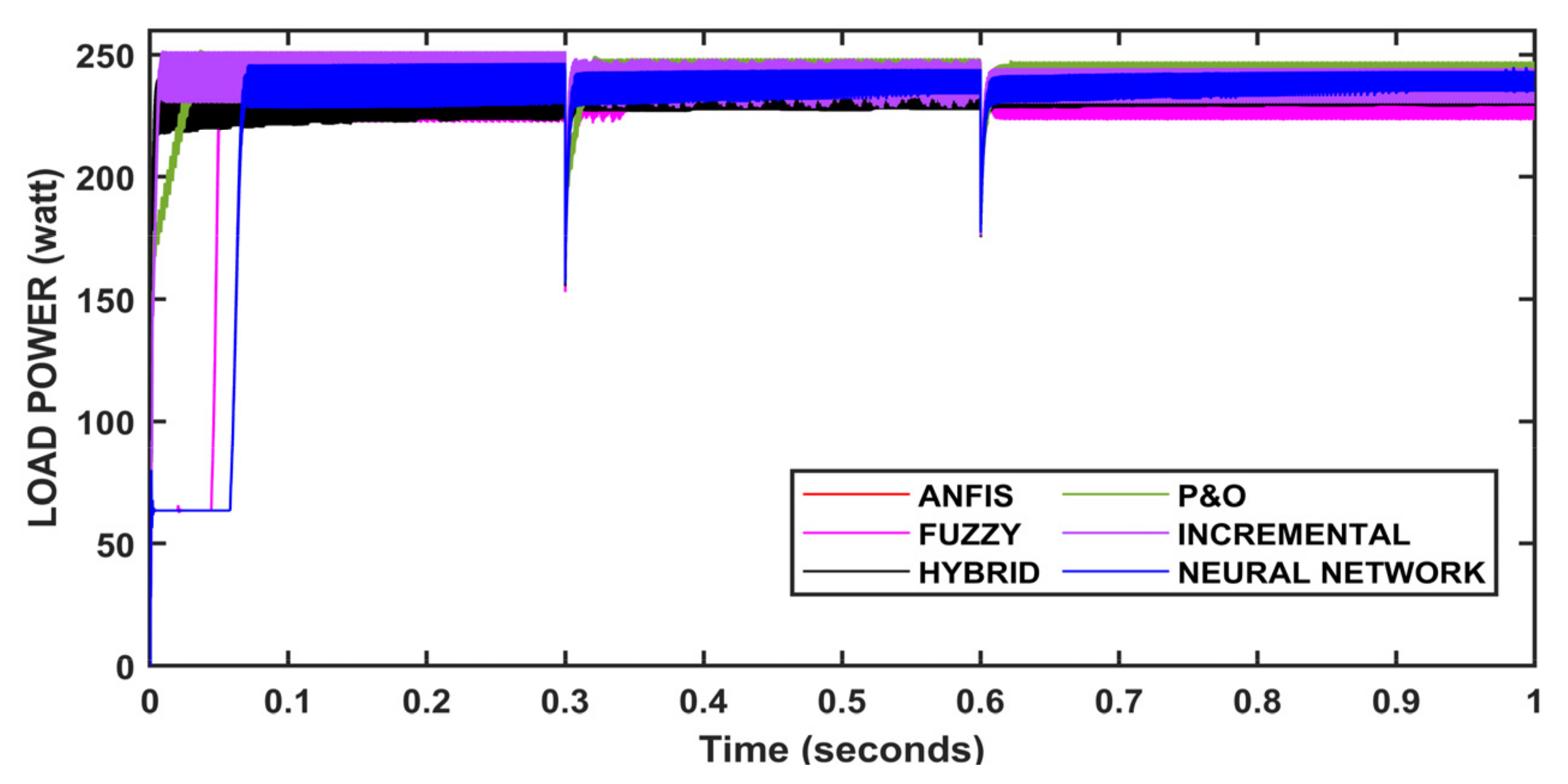
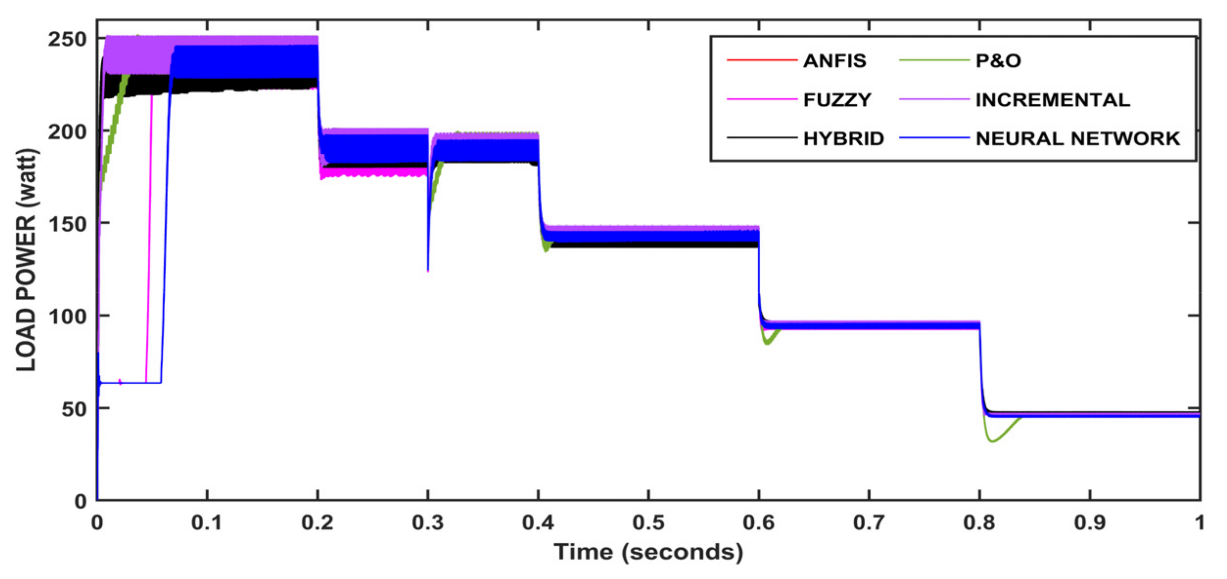
5. Results and Discussion

For changes in irradiation and temperature, the six investigated methods are compared. In standard conditions (under constant temperature, constant load, and a constant irradiance) Figure 43 demonstrates the transient behaviour of the tracked power out of six MPPT control systems. We observe that the hybrid controller achieves a steady state and MPP faster than the other controllers. The hybrid PV system’s steady-state behaviour is much more stable compared to the other MPPT techniques. The hybrid model significantly reduces power waste.
From the above simulation results of constant atmosphere, temperature, and load (Figure 43), we observe that the ANFIS and neural network output have overlapped each other. Figure 44 shows the performance of the PV system at variable loads and variable temperatures, using the six MPPT methods. The graph in Figure 45 depicts the performance of the six control schemes under constant illumination and varying loads. Figure 46 shows the controller performance at varying irradiations and varying loads. The simulation results demonstrate that the six controllers perform in a very similar manner in variable atmospheric conditions.
From the above figures for various temperatures, varying load, E = 1000 W/m2 (Figure 44), we can see that at the starting conditions, the output power is more than the panel’s maximum output power, and incremental has reached the maximum point first, followed by P&O, ANFIS, and fuzzy. The P&O and incremental algorithms were closer in the initial time, but at a few points, they overlapped. The neural network and hybrid algorithms have taken some time to track the maximum power point, although up to 0.4 s, these two algorithms’ outputs were lower than other algorithms. After the load disturbance at 0.3 s, the incremental gained MPP faster but was overtaken by P&O at 0.316 s, followed by fuzzy and ANFIS. After the disturbance at 0.6 s, the fuzzy gained first, which was closely followed by incremental and hybrid algorithms, and after 0.61 s, all algorithms performed in close proximity where P&O, neural network and hybrid, and ANFIS were leading. After 0.8 s disturbance, we observe that P&O, incremental, and fuzzy logic have overlapped in many instances, producing max output, followed by the hybrid algorithm. The neural network has lagged behind all four algorithms and ANFIS has lagged behind all the algorithms producing the least output.
From Figure 45, we can observe that the ANFIS and the neural network have overlapped each other. The hybrid was able to reach the MPP faster, followed by incremental, P&O, fuzzy logic, and ANFIS/neural network. After 0.3 s, it is the first disturbance showing that P&O and incremental have reached the MPP faster, followed by the hybrid algorithm, and neural network/ANFIS. Fuzzy logic had oscillated for a few cycles in the leading region/lagging region.
We can observe from the results that the neural network/ANFIS and hybrid methods gained the MPP faster with disturbances and have been in a steady state with fewer oscillations. The other algorithms such as P&O and incremental have a few more oscillations, and fuzzy has a greater amount of variations between the maximum and minimum positions.
From Figure 46 we can observe that incremental has reached the MPP faster, but the fast output was from the hybrid model, which was followed by P&O, fuzzy, and neural network/ANFIS. We can observe that the ANFIS and neural network have overlapped each other; we can see their outputs were very close. After 0.3 s, i.e., the first disturbance, we can see that the hybrid has gained MPP faster, followed by fuzzy, incremental, neural network/ANFIS, and P&O. P&O lagged behind all other algorithms. After 0.6 s, i.e., the second disturbance, we can observe that the hybrid gained faster, followed by incremental, neural network/ANFIS, fuzzy, and P&O. After 0.8 s, we can observe that the hybrid and the neural network gained faster compared to the others, but after reaching steady state, we can observe that the 0.966 hybrid was leading, followed by P&O, incremental, fuzzy, and ANFIS and neural network.
All the methods for various parametric variations are compared and tabulated in Table 5. In all the cases, the hybrid has maintained maximum and stable output.
From Table 6, we can observe that the hybrid model has good efficiency and more output power when compared to the other controllers, and the convergence time has been observed from simulations, the convergence time of P&O, with ANFIS being nearly the same, followed by incremental conductance and Fuzzy logic, the convergence time of NN, with hybrid models being the highest. As both the models were not tracking the MPP up to 0.02 s, but after 0.02 s they were able to track MPP better than other algorithms, the Hybrid model was able to converge faster than the other methods under varying conditions.
The models were simulated using MATLAB—R2020a, using an intel i3—10th generation based computer, and for the simulation time of 1 s, the models were tested for varying and constant conditions. The real-time required to simulate the model has been calculated. Under varying conditions of irradiation, the temperature and load time it took to simulate the model have been indicated in Table 7; for varying conditions, under constant conditions of irradiation, and the temperature and load time it took to simulate the model have been indicated in Table 7 as constant conditions. Therefore, we can observe under varying conditions and constant conditions that the P&O method had the lowest time followed by the hybrid and fuzzy logic control method, which required more time to simulate.

6. Conclusions

The results of all techniques used in this paper are compared, and examining the obtained results presented in the paper, it is clear that almost all of the techniques tracked MPP with sufficient accuracy. P&O has a very easy and simple implementation, but the system response oscillates across the MPP (ringing around) in steady-state operation, resulting in power waste. INC also has the same problems as P&O but has less amplitude of oscillations. The FLC is stable and has better fast-tracking of MPP, as compared with previous MPPT techniques in the paper. Under varying solar irradiance, FLC yielded good performance. FLC has advantages but it is more costly to implement with a slight efficiency advantage over the previous two algorithms.
An adaptive neuro-fuzzy inference system excels at tracking the maximum power point under varying irradiance and temperature conditions. The results from this MPPT technique performed better than FLC and previous methods in terms of robustness and performance, and reliability under varying irradiance levels.
In this article, an extremely-fast MPPT method that employs a combination of the NN method and the P&O method is compared with other methods. By reducing oscillations around the MPP and minimizing the perturbation and observation step times of the tracker, this modern hybrid method seemed to be able to enhance the performance of a traditional perturb and observe the algorithm. Extensive simulation and system results shed light on the algorithm’s behaviour. This showed a fast-tracking of the MPP, faster than traditional P&O.
Simulation results of the hybrid model show that the controller tracks MPP quickly in comparison with other controllers, and the hybrid method is very fast and precise in tracking MPP in varying atmospheric conditions. This method can extract maximum power and is efficient under varying atmospheric conditions. This method provides more power output than other methods, the transient response and steady-state response are quick and power losses are low as well.
As a result, this algorithm may be an ideal solution for massive PV farms where tracking time is critical. Furthermore, where the irradiance fluctuates abruptly, the hybrid approach will be an appealing solution. However, it needs to be acknowledged that for this technique to be very effective, the NN must be properly trained with a huge collection of datasets, which tends to make implementation difficult and expensive. Finally, specific applications may be worth the extra cost that this algorithm entails.
Based on the given varying parameters, the controllers gave a good performance and the hybrid model has maintained a stable point when compared with others, as other controllers suffered from ringing around the MPP, transient disturbances, and a slower settling time than the hybrid model. For normal applications where fast settling time is not required and cost-effectiveness is a matter of P&O, incremental is the best solution, but in the conditions where accuracy matters a lot, and the cost is not a criterion, fast response and low settling time are needed, and so, fuzzy, ANFIS and NN methods are considered important. Finally, it is concluded that the modern hybrid model has yielded satisfactory performance, according to the given variations.

7. Future Scope

There is a need for practical confirmation of the simulation results, as the convergence time, efficiency, and computational burdens in the practical implementations differ from that of the purely simulated results. In the papers [27,33,41], we can observe that the simulation results and the practical implementation results have a small amount of difference. Through practical implementations, we can come to know which methods are difficult to implement and which ones have high computational burdens on microcontrollers. In [14], we can find that fuzzy systems have high computational burdens. The practical devices also include additional losses and temperature dependency, so the outputs may differ from that of the simulation.
The researchers’ work, which included the design of an MPPT controller, should be expanded to track a wider variety of inputs that vary over time, such as system parameter variations. Recent mathematical models, such as z-infinity, can be used to obtain accurate MPPT points. The work done on the DC-DC converter is only limited by the use of a high-switching frequency.
However, the output power and THD values were not significantly improved, so further work in this area is required; the filter circuit design configuration must be improved. Converter circuits with grid interfacing have the issue that when a power failure occurs, the consumer cannot receive power even though the PV system is producing power. This should be treated as a serious issue, and research should be conducted in this area.

Author Contributions

Data curation, A.K.D. and N.K. and P.K.B.; Formal analysis, R.S. and T.S. (Tamilselvi Selvaraj); Funding acquisition, T.S. (Tomonobu Senjyu) and P.K.B.; Methodology, A.K.D. and N.K.; Project administration, P.K.B.; Resources, R.S., and T.S. (Tamilselvi Selvaraj); Supervision, T.S. (Tomonobu Senjyu); Writing–original draft, A.K.D. and N.K. All authors have read and agreed to the published version of the manuscript.

Funding

This research received no external funding.

Data Availability Statement

Not applicable.

Conflicts of Interest

The authors declare no conflict of interest.

References

  1. Beriber, D.; Talha, A. MPPT techniques for PV systems. In Proceedings of the 4th International Conference on Power Engineering, Energy and Electrical Drives, Istambul, Turkey, 13–17 May 2013; pp. 1437–1442. [Google Scholar] [CrossRef]
  2. Saleh, A.; Azmi, K.F.; Hardianto, T.; Hadi, W. Comparison of MPPT Fuzzy Logic Controller Based on Perturb and Observe (P&O) and Incremental Conductance (InC) Algorithm on Buck-Boost Converter. In Proceedings of the 2018 2nd International Conference on Electrical Engineering and Informatics (ICon EEI), Batam, Indonesia, 16–17 October 2018; pp. 154–158. [Google Scholar] [CrossRef]
  3. Selman, N.H. Comparison Between Perturb & Observe, Incremental Conductance and Fuzzy Logic MPPT Techniques at Different Weather Conditions. Int. J. Innov. Res. Sci. Eng. Technol. 2016, 5, 12556–12569. [Google Scholar] [CrossRef]
  4. Sridhar, R.; Jeevananathan, D.; Selvan, N.; Banerjee, S. Modeling of PV Array and Performance Enhancement by MPPT Algorithm. Int. J. Comput. Appl. 2010, 7, 35–39. [Google Scholar] [CrossRef]
  5. Zainudin, H.N.; Mekhilef, S. Comparison Study of Maximum Power Point Tracker Techniques for PV Systems. In Proceedings of the 14th International Middle East Power Systems Conference (MEPCON’10), Cairo, Egypt, 19–21 December 2010; pp. 750–755. [Google Scholar]
  6. Kalashani, M.B.; Farsadi, M. New Structure for Photovoltaic Systems with Maximum Power Point Tracking Ability. Int. J. Power Electron. Drive Syst. 2014, 4, 489. [Google Scholar] [CrossRef]
  7. Berrera, M.; Dolara, A.; Faranda, R.; Leva, S. Experimental Test of Seven Widely-Adopted MPPT Algorithms. In Proceedings of the 2009 IEEE Bucharest PowerTech, Bucharest, Romania, 28 June–2 July 2009; pp. 1–8. [Google Scholar] [CrossRef]
  8. Jyothy, L.P.; Sindhu, M.R. An Artificial Neural Network based MPPT Algorithm for Solar PV System. In Proceedings of the 2018 4th International Conference on Electrical Energy Systems (ICEES), Chennai, India, 7–9 February 2018; pp. 375–380. [Google Scholar] [CrossRef]
  9. Reisi, A.R.; Moradi, M.H.; Jamasb, S. Classification and comparison of maximum power point tracking techniques for photovoltaic system: A review. Renew. Sustain. Energy Rev. 2013, 19, 433–443. [Google Scholar] [CrossRef]
  10. Subudhi, B.; Pradhan, R. A Comparative Study on Maximum Power Point Tracking Techniques for Photovoltaic Power Systems. IEEE Trans. Sustain. Energy 2013, 4, 89–98. [Google Scholar] [CrossRef]
  11. Lee, H.-S.; Yun, J.-J. Advanced MPPT Algorithm for Distributed Photovoltaic Systems. Energies 2019, 12, 3576. [Google Scholar] [CrossRef]
  12. Khosrojerdi, F.; Taheri, S.; Cretu, A.-M. An adaptive neuro-fuzzy inference system-based MPPT controller for photovoltaic arrays. In Proceedings of the 2016 IEEE Electrical Power and Energy Conference (EPEC), Ottawa, ON, Canada, 12–14 October 2016; pp. 1–6. [Google Scholar] [CrossRef]
  13. Hijazi, R.; Karami, N. Neural Network Assisted Variable-Step-Size P&O for Fast Maximum Power Point Tracking. In Proceedings of the 2020 32nd International Conference on Microelectronics (ICM), Aqaba, Jordan, 14–17 December 2020; pp. 1–6. [Google Scholar] [CrossRef]
  14. Narendiran, S.; Sahoo, S.K.; Das, R.; Sahoo, A.K. Sahoo, Fuzzy logic controller based maximum power point tracking for PV system. In Proceedings of the 2016 3rd International Conference on Electrical Energy Systems (ICEES), Chennai, India, 17–19 March 2016; pp. 29–34. [Google Scholar] [CrossRef]
  15. Abdullah, G.; Aziz, M.S.; Hamad, B.A. Comparison between neural network and P&O method in optimizing MPPT control for photovoltaic cell. Int. J. Electr. Comput. Eng. 2020, 10, 5083–5092. [Google Scholar] [CrossRef]
  16. Sarvi, M.; Azadian, A. A comprehensive review and classified comparison of MPPT algorithms in PV systems. Energy Syst. 2021, 13, 281–320. [Google Scholar] [CrossRef]
  17. Atri, P.K.; Modi, P.S.; Gujar, N.S. Comparison of Different MPPT Control Strategies for Solar Charge Controller. In Proceedings of the 2020 International Conference on Power Electronics & IoT Applications in Renewable Energy and its Control (PARC), Mathura, India, 28–29 February 2020; pp. 65–69. [Google Scholar] [CrossRef]
  18. Chtouki, I.; Wira, P.; Zazi, M. Comparison of Several Neural Network Perturb and Observe MPPT Methods for Photovoltaic Applications. In Proceedings of the 2018 IEEE International Conference on Industrial Technology (ICIT), Lyon, France, 20–22 February 2018; pp. 909–914. [Google Scholar] [CrossRef]
  19. Khosravi, M.; Heshmatian, S.; Khaburi, D.A.; García, C.; Rodríguez, J. A Novel Hybrid Model-Based MPPT Algorithm Based on Artificial Neural Networks for Photovoltaic Applications. In Proceedings of the 2017 IEEE Southern Power Electronics Conference (SPEC), Puerto Varas, Chile, 4–7 December 2017; pp. 1–6. [Google Scholar] [CrossRef]
  20. Dahiya, A.K. Implementation and Comparison of Perturb & Observe, ANN and ANFIS Based MPPT Techniques. In Proceedings of the 2018 International Conference on Inventive Research in Computing Applications (ICIRCA), Coimbatore, India, 11–12 July 2018; pp. 1–5. [Google Scholar] [CrossRef]
  21. Kacimi, N.; Grouni, S.; Idir, A.; Boucherit, M.S. New improved hybrid MPPT based on neural network-model predictive control-kalman filter for photovoltaic system. Indones. J. Electr. Eng. Comput. Sci. 2020, 20, 1230–1241. [Google Scholar] [CrossRef]
  22. Kanimozhi, K.; Rabi, B.R.M. Development of Hybrid MPPT Algorithm for Maximum Power Harvesting under Partial Shading Conditions. Circuits Syst. 2016, 7, 1611–1622. [Google Scholar] [CrossRef] [Green Version]
  23. Bataineh, K. Improved hybrid algorithms-based MPPT algorithm for PV system operating under severe weather conditions. IET Power Electron. 2019, 12, 703–711. [Google Scholar] [CrossRef]
  24. Aurilio, G.; Balato, M.; Graditi, G.; Landi, C.; Luiso, M.; Vitelli, M. Fast Hybrid MPPT Technique for Photovoltaic Applications: Numerical and Experimental Validation. Adv. Power Electron. 2014, 2014, 125918. [Google Scholar] [CrossRef]
  25. Sarwar, S.; Javed, M.Y.; Jaffery, M.H.; Arshad, J.; Rehman, A.U.; Shafiq, M.; Choi, J.-G. A Novel Hybrid MPPT Technique to Maximize Power Harvesting from PV System under Partial and Complex Partial Shading. Appl. Sci. 2022, 12, 587. [Google Scholar] [CrossRef]
  26. Bollipo, R.B.; Mikkili, S.; Bonthagorla, P.K. Hybrid, optimization, intelligent and classical PV MPPT techniques: A Review. CSEE J. Power Energy Syst. 2021, 7, 9–33. [Google Scholar] [CrossRef]
  27. Azzouz, S.; Messalti, S.; Harrag, A. A Novel Hybrid MPPT Controller Using (P&O)-neural Networks for Variable Speed Wind Turbine Based on DFIG. Model. Meas. Control A 2019, 92, 23–29. [Google Scholar] [CrossRef]
  28. Arjun, M.; Zubin, J.B. Artificial Neural Network Based Hybrid MPPT for Photovoltaic Modules. In Proceedings of the 2018 International CET Conference on Control, Communication, and Computing (IC4), Thiruvananthapuram, India, 5–7 July 2018; pp. 140–145. [Google Scholar] [CrossRef]
  29. Sher, H.A.; Murtaza, A.F.; Noman, A.; Addoweesh, K.E.; Al-Haddad, K.; Chiaberge, M. A New Sensorless Hybrid MPPT Algorithm Based on Fractional Short-Circuit Current Measurement and P&O MPPT. IEEE Trans. Sustain. Energy 2015, 6, 1426–1434. [Google Scholar] [CrossRef] [Green Version]
  30. Pakkiraiah, G.B.; Durga, S. Research Survey on Various MPPT Performance Issues to Improve the Solar PV System Efficiency. J. Sol. Energy 2016, 2016, 8012432. [Google Scholar] [CrossRef] [Green Version]
  31. Bhukya, L.; Kedika, N.R.; Salkuti, S.R. Enhanced Maximum Power Point Techniques for Solar Photovoltaic System under Uniform Insolation and Partial Shading Conditions: A Review. Algorithms 2022, 15, 365. [Google Scholar] [CrossRef]
  32. Javed, M.R.; Waleed, A.; Virk, U.S.; Hassan, S.Z.U. Comparison of the Adaptive Neural-Fuzzy Interface System (ANFIS) based Solar Maximum Power Point Tracking (MPPT) with other Solar MPPT Methods. In Proceedings of the 2020 IEEE 23rd International Multitopic Conference (INMIC), Bahawalpur, Pakistan, 5–7 November 2020; pp. 1–5. [Google Scholar] [CrossRef]
  33. Singh, M.D.; Shine, V.J.; Janamala, V. Application of Artificial Neural Networks in Optimizing MPPT Control for Standalone Solar PV System. In Proceedings of the 2014 International Conference on Contemporary Computing and Informatics (IC3I), Mysore, India, 27–29 November 2014; pp. 162–166. [Google Scholar] [CrossRef]
  34. Khanam, J.; Foo, S.Y. Neural Networks Technique for Maximum Power Point Tracking of Photovoltaic Array. In Proceedings of the SoutheastCon, St. Petersburg, FL, USA, 19–22 April 2018; pp. 1–4. [Google Scholar] [CrossRef]
  35. Hayder, W.; Sera, D.; Ogliari, E.; Lashab, A. On Improved PSO and Neural Network P&O Methods for PV System under Shading and Various Atmospheric Conditions. Energies 2022, 15, 7668. [Google Scholar] [CrossRef]
  36. Dagal, I.; Akın, B.; Akboy, E. MPPT mechanism based on novel hybrid particle swarm optimization and salp swarm optimization algorithm for battery charging through simulink. Sci. Rep. 2022, 12, 2664. [Google Scholar] [CrossRef] [PubMed]
  37. Ali, Z.M.; Alquthami, T.; Alkhalaf, S.; Norouzi, H.; Dadfar, S.; Suzuki, K. Novel hybrid improved bat algorithm and fuzzy system based MPPT for photovoltaic under variable atmospheric conditions. Sustain. Energy Technol. Assess. 2022, 52, 102156. [Google Scholar] [CrossRef]
  38. Gong, L.; Hou, G.; Huang, C. A two-stage MPPT controller for PV system based on the improved artificial bee colony and simultaneous heat transfer search algorithm. ISA Transactions 2022. [Google Scholar] [CrossRef]
  39. Manna, S.; Akella, A.K.; Singh, D.K. A Novel MRAC-MPPT Scheme to Enhance Speed and Accuracy in PV Systems. Iran. J. Sci. Technol. Trans. Electr. Eng. 2022. [Google Scholar] [CrossRef]
  40. Manna, S.; Singh, D.K.; Akella, A.K.; Abdelaziz, A.Y.; Prasad, M. A novel robust model reference adaptive MPPT controller for Photovoltaic systems. Sci. Iran. 2022. [Google Scholar] [CrossRef]
  41. Badoud, A.E.; Mekhilef, S.; Bouamama, B.O. A Novel Hybrid MPPT Controller Based on Bond Graph and Fuzzy Logic in Proton Exchange Membrane Fuel Cell System: Experimental Validation. Arab. J. Sci. Eng. 2021, 47, 3201–3220. [Google Scholar] [CrossRef]
Figure 1. Electrical equivalent of the solar cell.
Energies 15 08776 g001
Figure 2. P-V curve for different temperatures at 1000 W/m2 irradiation.
Energies 15 08776 g002
Figure 3. I-V, P-V curves for various irradiations at 25 °C.
Energies 15 08776 g003
Figure 4. Schematic of the DC-DC boost converter.
Energies 15 08776 g004
Figure 5. MPPT control for the PV system.
Energies 15 08776 g005
Figure 6. dp/dv sign at various points of the curve [11].
Energies 15 08776 g006
Figure 7. Flowchart for P&O algorithm.
Energies 15 08776 g007
Figure 8. The effect of perturbation step size on the behaviour of the P&O method.
Energies 15 08776 g008
Figure 9. Algorithm performance at constant atmospheric conditions; T = 25 °C, w = 1000 W/m2, R = 10 Ω.
Energies 15 08776 g009
Figure 10. Algorithm performance at variable irradiations and variable loads; T = 25 °C.
Energies 15 08776 g010
Figure 11. Algorithm performance at variable loads; T = 25 °C, w = 1000 W/m2.
Energies 15 08776 g011
Figure 12. Algorithm performance at variable temperatures and variable loads; w = 1000 W/m2.
Energies 15 08776 g012
Figure 13. Slope at various regions of the PV curve [6].
Energies 15 08776 g013
Figure 14. Algorithm performance under varying loads, and constant temperature and irradiation.
Energies 15 08776 g014
Figure 15. Algorithm performance under constant irradiation, load, and temperature.
Energies 15 08776 g015
Figure 16. Algorithm performance under variable irradiations and varying loads.
Energies 15 08776 g016
Figure 17. Algorithm performance under variable temperatures and varying loads.
Energies 15 08776 g017
Figure 18. Block diagram of fuzzy control.
Energies 15 08776 g018
Figure 19. Flowchart of the fuzzy logic system.
Energies 15 08776 g019
Figure 20. Error, change in error, and duty cycle membership functions of fuzzy inference system: (a) membership functions of input variable Ipv; (b) membership functions of input variable Vpv; (c) membership functions of output variable PWM (or) duty.
Energies 15 08776 g020aEnergies 15 08776 g020b
Figure 21. FLC output power under constant irradiations and variable loads.
Energies 15 08776 g021
Figure 22. Output power of FLC system at constant load, temperature, and irradiance.
Energies 15 08776 g022
Figure 23. Algorithm performance under variable irradiations and varying loads.
Energies 15 08776 g023
Figure 24. Algorithm performance under variable temperatures and variable loads.
Energies 15 08776 g024
Figure 25. Neural network training: (a) NNTOOL for NN training in MATLAB; (b) performance plot of neural network; (c) training state plot; (d) error histogram; (e) regression plot; (f) results of trained data.
Energies 15 08776 g025aEnergies 15 08776 g025b
Figure 26. Flow chart of neural network MPPT.
Energies 15 08776 g026
Figure 27. Output power of NN system at variable loads and constant irradiation and temperature.
Energies 15 08776 g027
Figure 28. Output power of NN system at constant irradiance, temperature, and load.
Energies 15 08776 g028
Figure 29. Output power of NN system at variable loads and variable irradiances.
Energies 15 08776 g029
Figure 30. Output power of NN system at variable temperatures and varying loads.
Energies 15 08776 g030
Figure 31. ANFIS Architecture for Time Series Modeling.
Energies 15 08776 g031
Figure 33. Performance at variable loads and constant irradiation and temperature.
Energies 15 08776 g033
Figure 34. Performances at constant irradiance, temperature, and load.
Energies 15 08776 g034
Figure 35. Performance at variable loads and varying irradiances.
Energies 15 08776 g035
Figure 36. Performance at variable temperatures and varying loads.
Energies 15 08776 g036
Figure 37. Block diagram of the hybrid model [21,22,23].
Energies 15 08776 g037
Figure 38. Flow chart for hybrid MPPT based on neural network and P&O [23].
Energies 15 08776 g038
Figure 39. Performance at variable loads and constant irradiation and temperature.
Energies 15 08776 g039
Figure 40. Performances at constant irradiance, temperature, and load.
Energies 15 08776 g040
Figure 41. Performance at variable loads and varying irradiances.
Energies 15 08776 g041
Figure 42. Performance at variable temperatures and variable loads.
Energies 15 08776 g042
Figure 43. Controllers’ performance for constant irradiance; 1000 W/m2, T = 25 °C, load = 30 Ω.
Energies 15 08776 g043
Figure 44. Controller performance at various temperatures and varying loads; E = 1000 W/m2.
Energies 15 08776 g044
Figure 45. Controller performance at constant irradiation and varying loads.
Energies 15 08776 g045
Figure 46. Controller performance at varying irradiations and varying loads.
Energies 15 08776 g046
Table 1. Parameters and specifications of PV module.
ParameterSpecifications
Maximum power250.20 W
Open circuit voltage37.3 V
Voltage at maximum power point30.7 V
Short circuit current8.66 A
Current at maximum power point8.15 A
Table 2. Table showing the variation of parameters.
ParameterTime (sec)Value
Irradiance(0, 0.2, 0.4, 0.6, 0.8)(1000, 800, 600, 400, 200) w/m2
Temperature
Load
(0, 0.2, 0.4, 0.6, 0.8)
(0, 0.3, 0.6)
(−15, 10, 25, 30, 45) Celsius
(20, 30, 40) Ω
The above parameter variations are applied to all other MPPT methods.
Table 3. Fuzzy control rule base.
d v / d p NBNSZEPSPB
NBPBPSNBNSNS
NSPSPSNBNSNS
ZENSNSNSPBPB
PSNSPBPSNBPB
PBNBNBPBPSPB
Table 4. Particulars in neural network training.
SpecificationsDataValidation and Test Data
of 1000 Samples
ToolboxNNTOOL boxType of
Sample
Samples
(%)
Total Samples
Wizard: Input-output
and curve fitting
Fitting appTraining 70%700
samples
Input data to network1000 points input data of
irradiation, temperature
Validation15%150
samples
Target data/desired
network output
1000 points data of voltageTesting15%150
samples
Samples Matrix—rows
Number of hidden neurons 10
Training AlgorithmLevenberg–Marquardt
Table 5. Comparison of various methods in various parameters.
ItemsP&O
Method
Incremental Conductance MethodFuzzy Logic Control MethodANFIS MethodNeural
Network Method
Hybrid
Controller Model
Dynamic behaviourPoorMediumMediumGoodGoodFast
Transient behaviourBadBadGoodGoodGoodFast
(oscillations) Steady-stateLargeModerateSmallSmallSmallVery small
requirementsP&O
algorithm
Incremental conductance
algorithm
Fuzzy
logic
membership
functions
ANFIS
training
data
Neural
network training
data
Neural
network and P&O
combined
Static errorHighHighLowLowLowlow
Controller accuracyLowMediumAccurateAccurateAccurateAccurate
Tracking speedSlowSlowFastFastFastFaster
System complexitySimple power calculationsSimpleMediumMediumMediumMedium
Temperature characteristicsPoorPoorGoodGoodGoodBetter
Parameters tuningNoNoYesYesYesYes
Table 6. Average power, convergence time, and efficiencies for various methods.
MPPT MethodConvergence
Time(s)
Irradiation: 1000 w/m2ValuesComment
P_max: 250 w/m2
P&O method0.004P_avg237.4Oscillations occur
PV94.96
Incremental
Conductance method
0.006P_avg239.1Oscillations occur
PV95.60
Fuzzy logic control
method
0.04P_avg242.2Long convergence time
PV96.88
Neural network
method
0.205P_avg244.6Better dynamic performance
PV97.84
ANFIS control
method
0.046P_avg244.4Under dynamic response
PV97.76
Hybrid Method0.2005P_avg247Fast response
PV98.80
Table 7. Computational burden of MPPT methods.
Method NameReal-Time (s)
(Varying Conditions)
Real-Time (s)
(Constant Conditions)
P&O4.6333.875
Incremental conductance9.26355.771
Fuzzy logic control423.88372.41
Neural network7.7014.6345
ANFIS50.559541.07
Hybrid6.1545.667
Publisher’s Note: MDPI stays neutral with regard to jurisdictional claims in published maps and institutional affiliations.

