
Overview of the Fundamentals and Applications of Bifacial Photovoltaic Technology: Agrivoltaics and Aquavoltaics

Abstract
:1. Introduction
2. Bifacial PV Technology
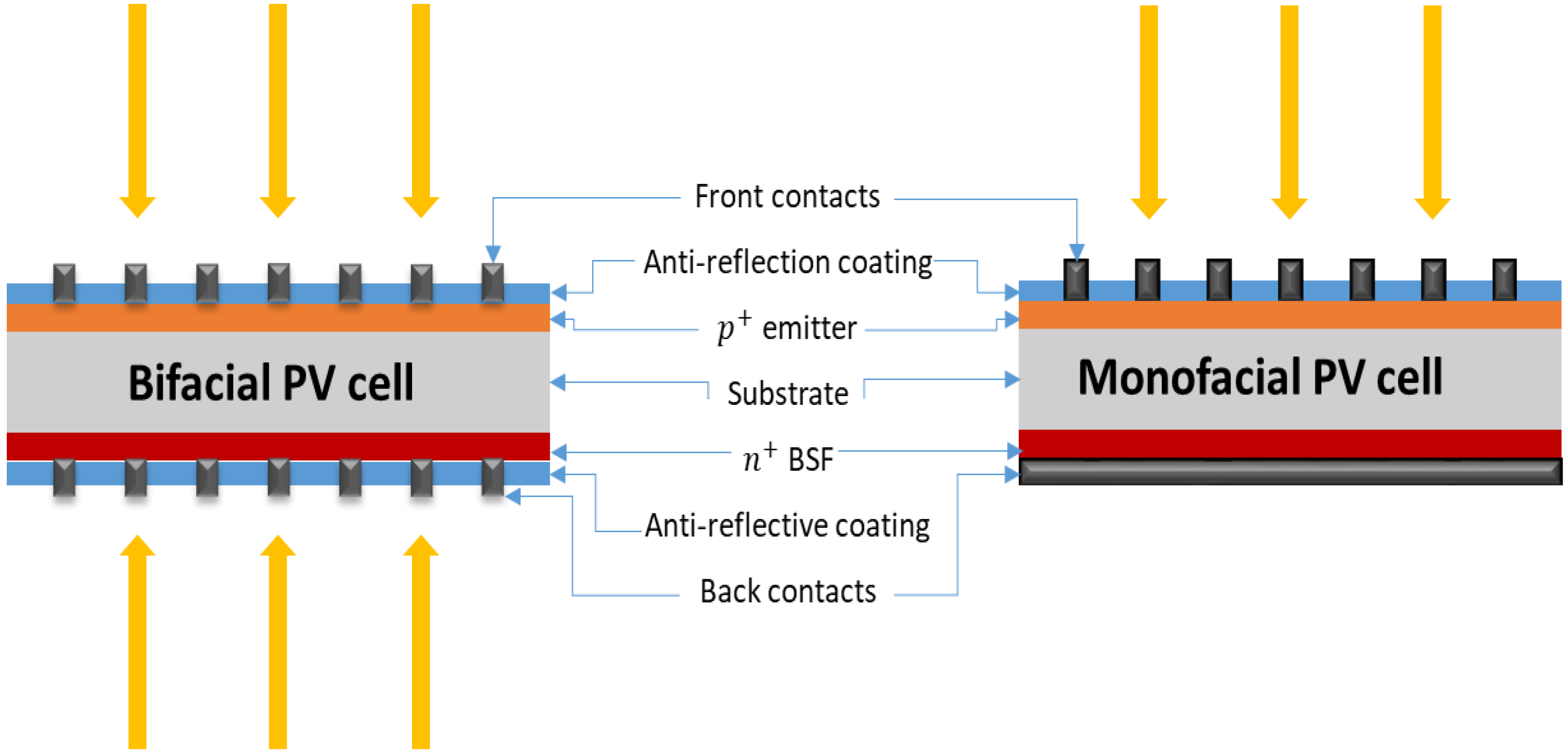
2.1. Bifacial PV Cells
2.2. Fundamental Solar Cell Losses
- Carrier transportation process losses consist mainly of: (i) series resistance losses, due to the loss in the transport of carriers in their paths due to collision with atoms or other carriers [26]; (ii) the shunt resistance loss can be associated with the recombination process, which conducts the generation of heat and is proportional to the loss of photocurrent; [27](iii) The Carnot loss is defined as the minimum energy required to separate photo-generated charges [26]; and (iv) the angular mismatch loss referred to the energy loss caused by the mismatch between the absorption and emission solid angles [24].
- Carrier recombination process losses: emission loss corresponds to the photons emitted by the cells resulting from radiative recombination and non-radiative recombination loss [24].
2.3. Bifacial Technology Performance Parameters
- The power conversion efficiency () is the ratio of the generated electrical power Pm (W) to the incident light power E (W/m2) under one sun with a ( = 1000 W/m2) or more. It is measured separately for the front and rear faces. In general, it is calculated at the maximum power point, Pm, in W, using the area of the solar cell (A, in m2). This definition can extend to define the bifacial module efficiency as the power produced divided by the total irradiance power received by the working surfaces of the module. The efficiency of the bPV cell can go from 19.4% for PERC to 24.7% for HIT at the front side, and from 16.7% for PERC to 19% for PERT at the rear side (Figure 2) [5].
- The bifaciality factor () defines the ratio of the device’s front and rear responses under the same conditions. This parameter essentially determines the additional power that can be generated by the rear irradiance. In the literature, there are different approaches to defining the bifaciality factor, based on power, current density, voltage, or efficiency. The most common one is the ratio between the power of the rear of the module and the front under STC conditions [8]. The main equations to define bifaciality are as follows:where is the current density, the voltage, and the power and ƞ the efficiency. The subscripts “f” and “r” indicate the front and rear surfaces, respectively. The main characteristics that determine the bifaciality factor of a bPV cell are the rear surface texture and antireflection coating (ARC) [28,29], the metal coverage of the rear side contact [30], the rear side back surface field (BSF) doping and passivation [31], and the base resistivity and lifetime of the solar cell [32]. The maximum bifaciality factor was achieved for Si heterojunction bPV cells with values ranging from 85 to 95%, followed by n-PERT from 75 to 90%, and then by the P-PERC from 65 to 80% [8].
- The bifacial gain (BG): an appropriate way to illustrate the importance of bifaciality is to analyze the bifacial gain, which is defined as the difference in energy yield when comparing bifacial and monofacial devices with identical installation configurations. Generally, this comparison is based on the energy yield, expressed in KWh/KWp [33].where is the energy yield of a PV system with bifacial modules and the energy yield with monofacial modules in the same conditions (site, configuration, and time period). A similar factor is the bifacial optical gain in Equation (7), which is defined as the ratio of the rear ( to the front () irradiances [34]. The bifacial gain depends mainly on the ground albedo and the distance between rows. The smaller the distance between the module rows, the lower the BG, and a high albedo will result in a higher BG [34].
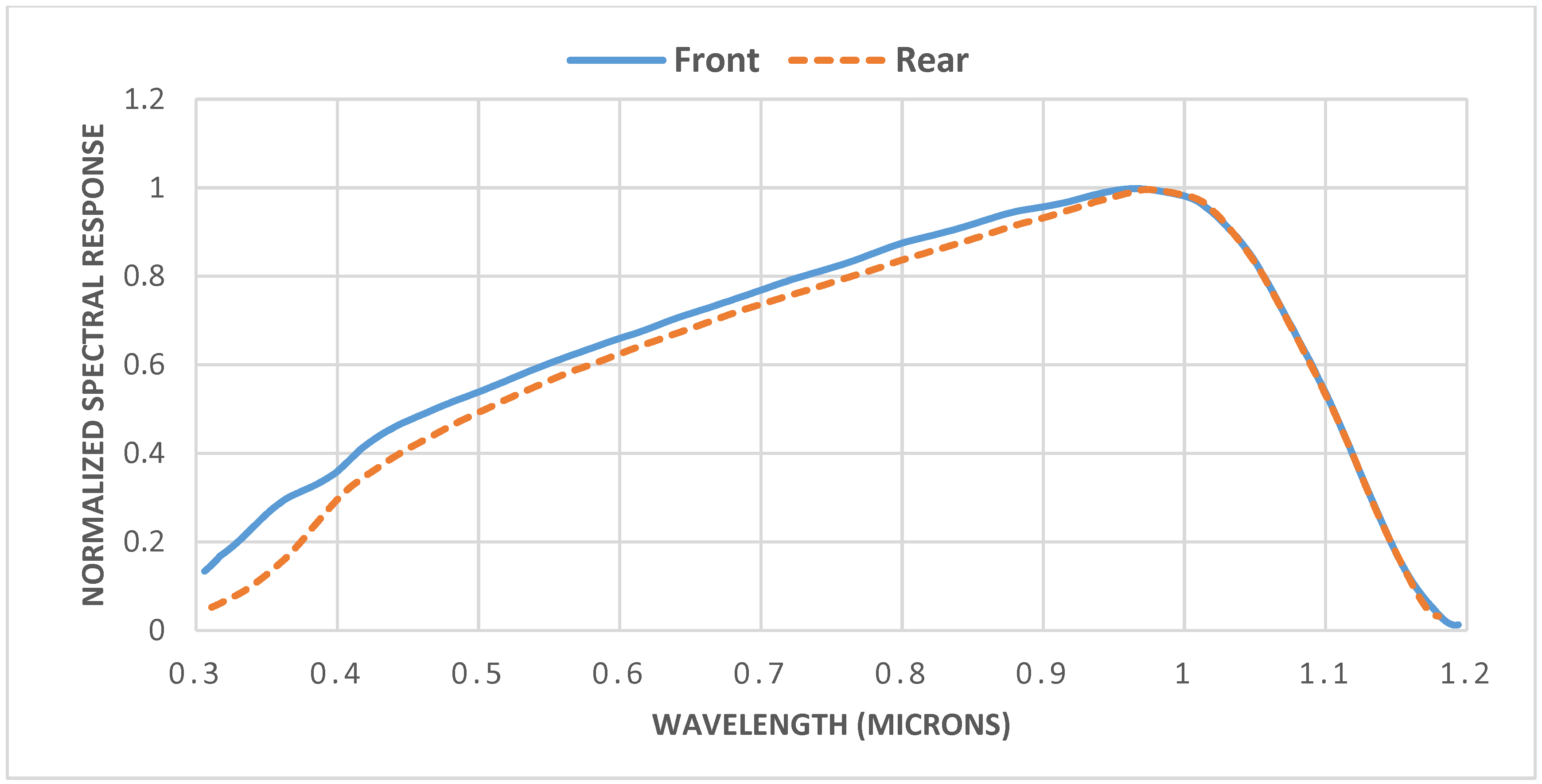
- The spectral response (SR): as the monofacial cells photovoltaic cells, bPV cells have a spectral response (SR in A/W) representing the fraction of the available irradiance that is converted to current [35]. The front and rear of the bPV cell may show a slight difference in spectral response (Figure 4) [36], mainly due to the difference between the two sides in passivation and metal contacts.
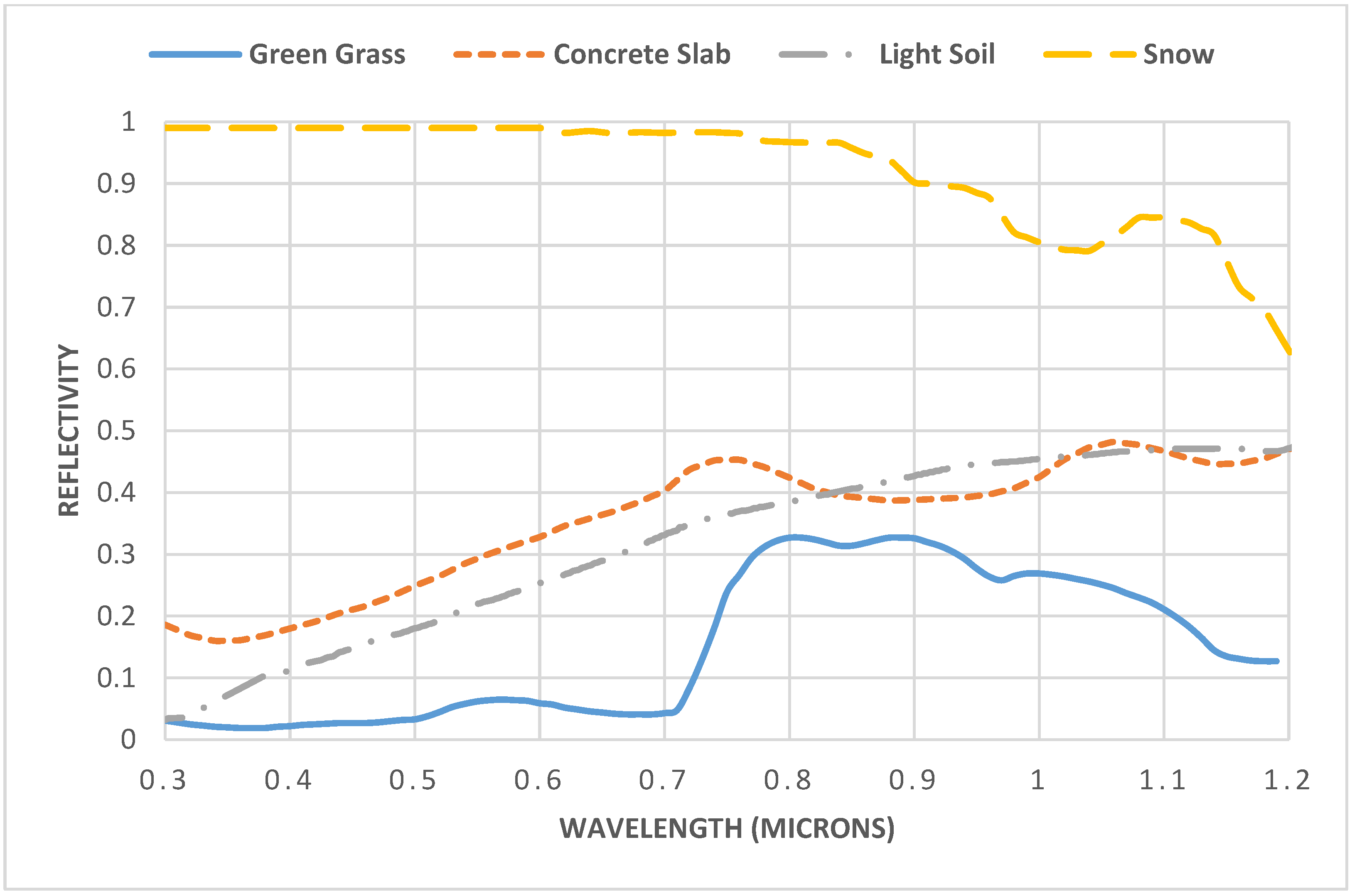
- The ground albedo (): ratio of reflected radiation to the radiation from the sky dome. It is common to assume the albedo of the ground surface as a constant for monofacial PV systems, due to the limited contribution of reflected irradiation from the ground. In general, the contribution of reflected radiation on the ground is less than 3% for most monofacial PV systems and can be less than 1% for systems with a slope of less than 25° [33]. In fact, the albedo is spectral and angle-dependent, and because of the significant rear reflected irradiance importance for bPV systems, the spectral albedo is typically adopted (Figure 5). The constant percentage of reflected light α can be calculated as a function of spectral reflectivity (λ) as [37]:where G(λ) is the spectrum incident on the surface. The reflected light can be simply calculated by multiplying the constant albedo by the broadband incident spectrum at this point.
3. b-PV Modeling Methods
3.1. Optical
3.1.1. Front-Side Irradiance
3.1.2. Rear-Side Irradiance
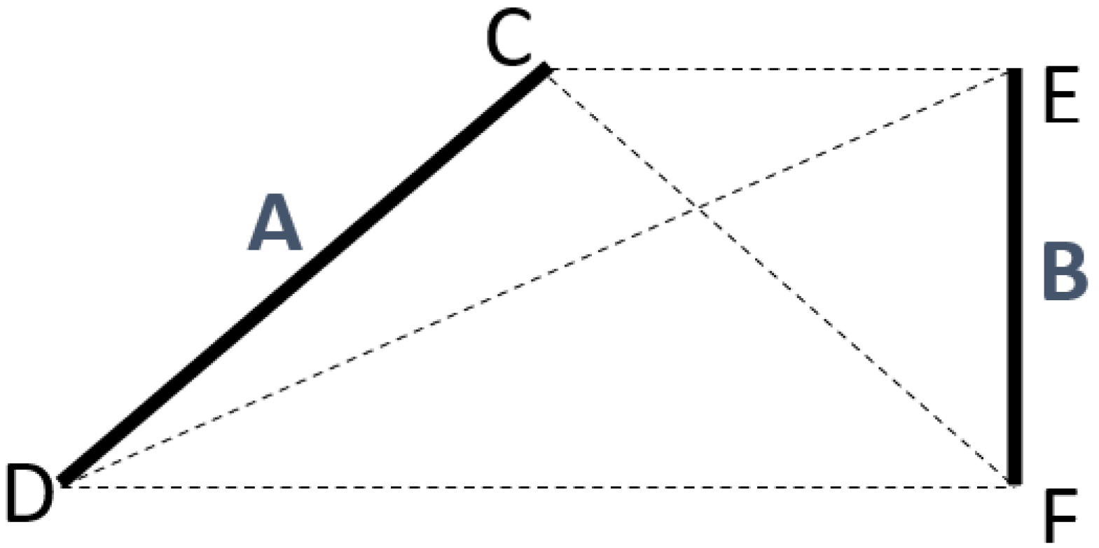
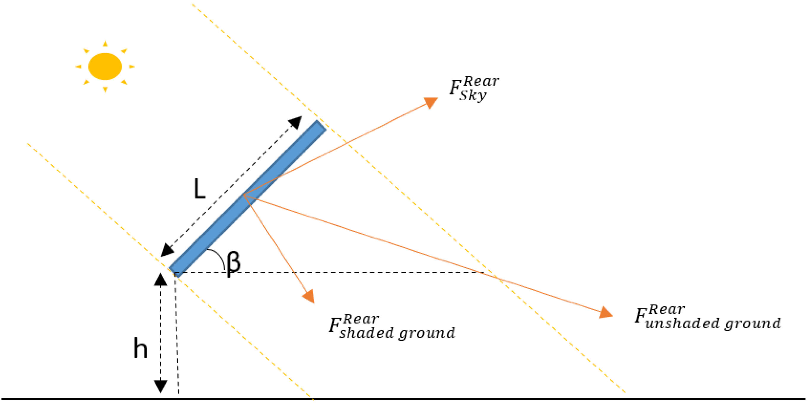
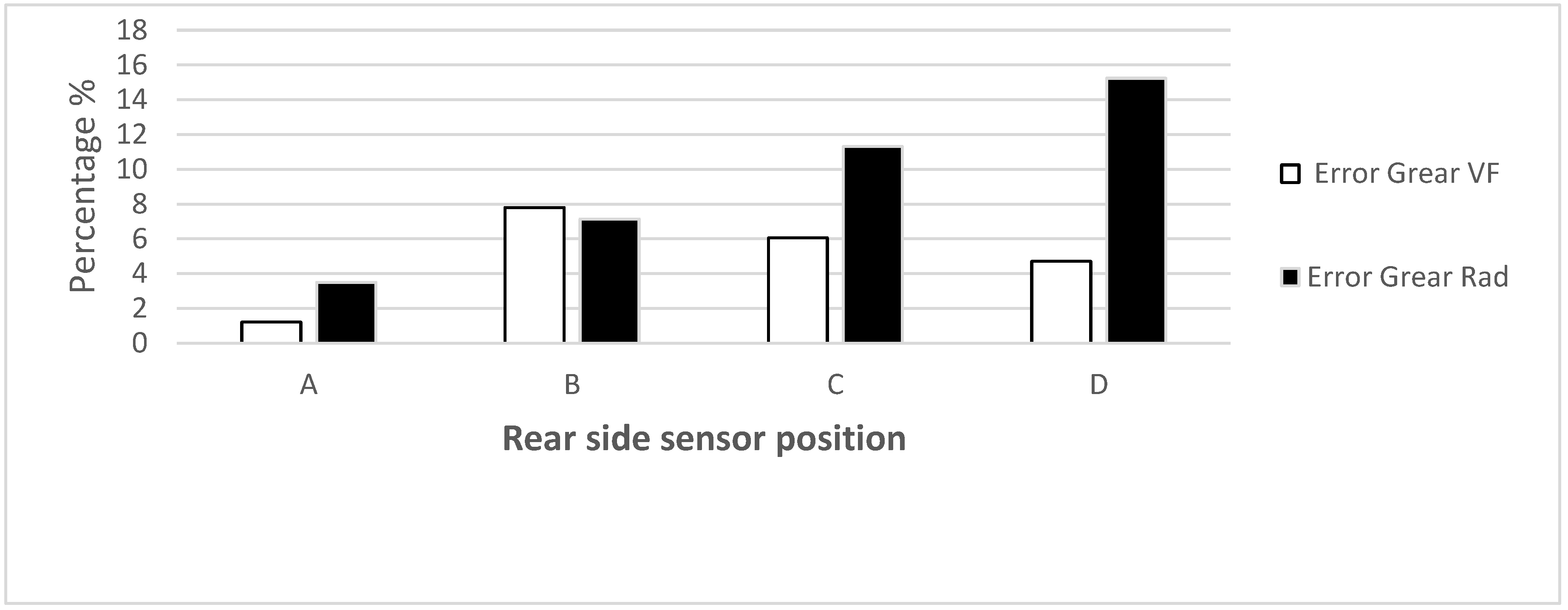
The View Factor Model
Ray Tracing Model
3.2. Electrical
3.2.1. Single Point Power Model
3.2.2. Characteristic Point Model
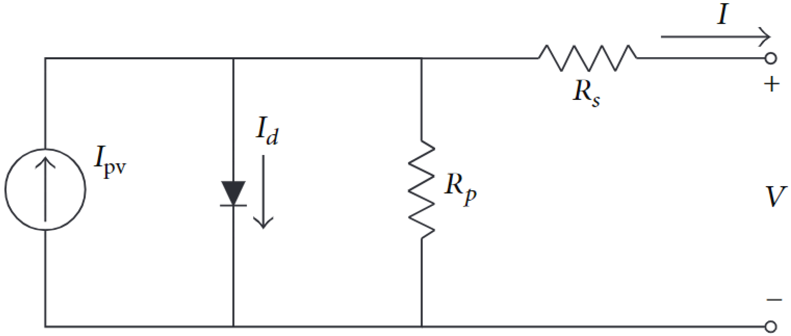
3.2.3. Equivalent Circuit Model
3.3. Thermal
3.3.1. NOCT Model
3.3.2. Sandia Model
3.3.3. PVsyst Model
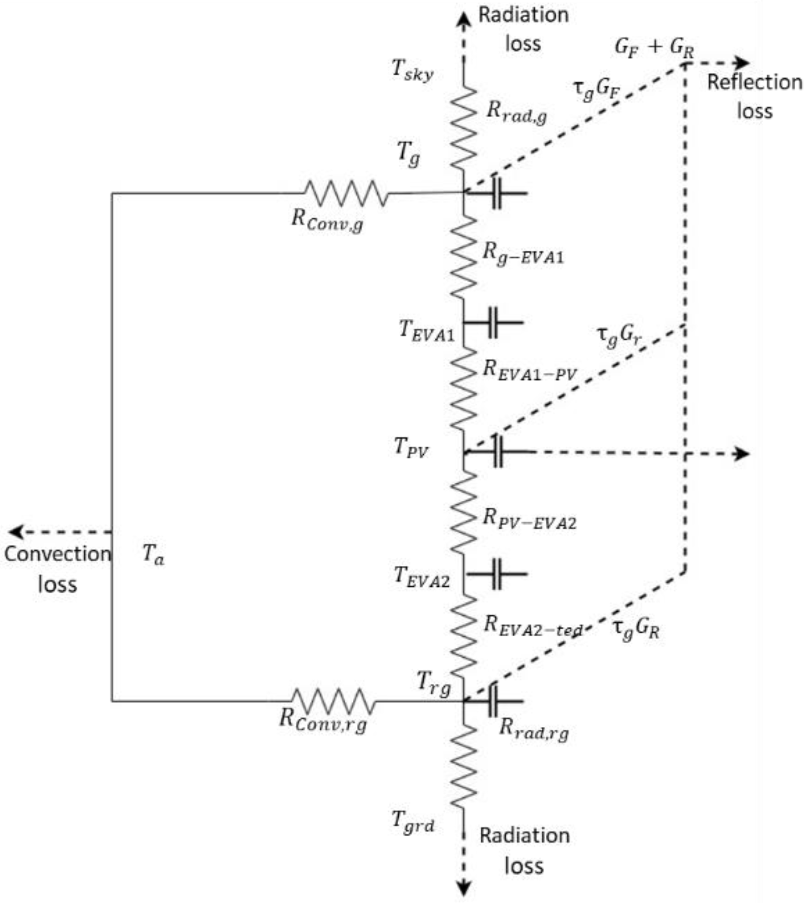
3.3.4. Equivalent Thermal Circuit Model
3.3.5. Regression Model
4. Bifacial Technology Applications
4.1. Agrivoltaic
4.1.1. APV Main Parameters
4.1.2. Bifacial APV Configurations
Single Axis Tracking Configuration
Fixed Tilt Configuration
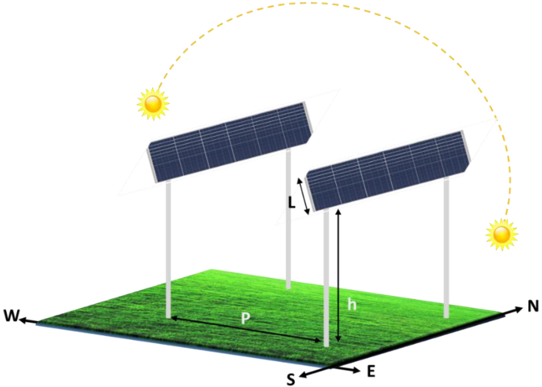
The Pitch Distance
The Elevation

| No | Location | Electricity Yield | Capacity | PV Tracking | Cultivated Crops | Technology | Further Information | Refs |
|---|---|---|---|---|---|---|---|---|
| 1 | Donaueschingen—Aasen, Germany | 4850 MWh/year | 4.1 MWp | No | Meadow used for hay and silage | N-Pert (100%) | It is the largest bifacial agrivoltaic system in Europe. Was put into operation in 2020 and supplies electricity to 1400 households. | [107] |
| 2 | Eppelborn—Saarland, Germany | 2150 MWh/year | 2 MWp | No | Meadow used for hay and silage | N-Pert (60%), Heterojunction (40%) | It is the first large-scale bifacial PV system in Europe. It was launched in 2018 and supplies electricity to 700 households. | [107] |
| 3 | Channay, France | 265 MWh/year | 237 KWp | No | Test site for different arable crops and cattle farming | n-Type PERT/Heterojunction Bifacial Frameless | It is one of the first vertical bifacial agricultural power plants in France. It was put into operation in 2021 and supplies electricity to 80 households. | [107] |
| 4 | Valpuiseaux, France | 124 MWh/year | 111 KWp | No | Test site for different arable crops and cattle farming | n-Type PERT/Heterojunction Bifacial Frameless | It was put into operation in 2021 to supply electricity to 40 households. | [107] |
| 5 | Mälardalen University, Västerås, Sweden | 37 MWh/year | 33 KWp | No | Test site for different arable crops | n-Type PERT Bifacial Frameless | It was the first bifacial agrivoltaic farm in Sweden. It was put into operation in 2021 and supplies electricity to 11 households. | [107] |
| 6 | Seongang, South Korea | 1300 KWh/year | 30 KWp | No | No information | N-Pert (100%) | This is South Korea’s first agrivoltaic plant, which started operating in 2020. | [107] |
| 7 | Saarland, Germany | 31 MWh/year | 28 KWp | No | Pastureland | Bifacial n-type cells | This is a pilot plant used for the validation of Next2Sun’s vertical assembly system; launched in 2015. | [107] |
| 8 | Guntramsdorf, Austria | 23 MWh/year | 22.5 KWp | No | Arable land for the cultivation of potatoes | N-Pert (100%) | Austria’s first ground-mounted agricultural photovoltaic-photovoltaic plants. It started in 2019. | [107] |
| 9 | Heggelbach, Germany | 245 MWh/year | 194 KWp | No | Winter wheat, potatoes, celery, and clover grass | No information | This project supplies electricity to 62 households and the preliminary result of the project showed an increase in the LER by more than 60%. | [108] |
| 10 | Bierbeek, Belgium | No information | 185 W | One-axis solar tracking and fix tilt set-ups | Orchard crops, and pear trees | C-Si cells with transparent backsheet | Started in 2021; designed to demonstrate the viability of agrivoltaics in Belgium | [109] |
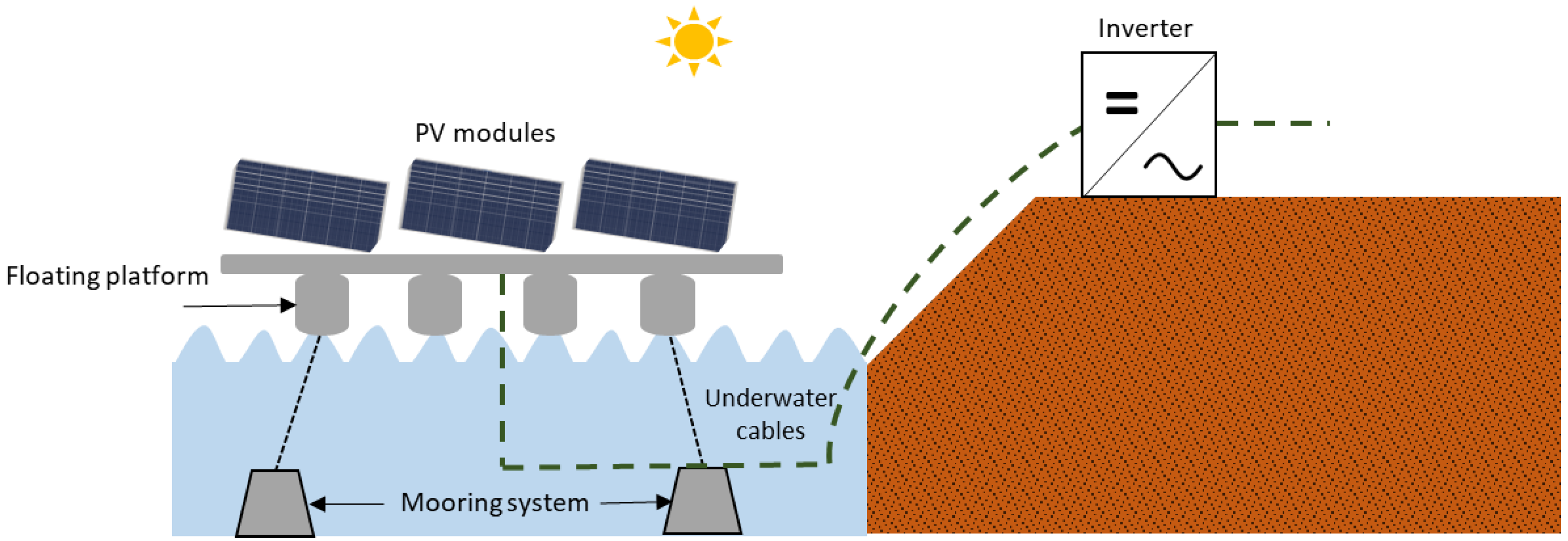
4.2. Floating (Aquavoltaic)
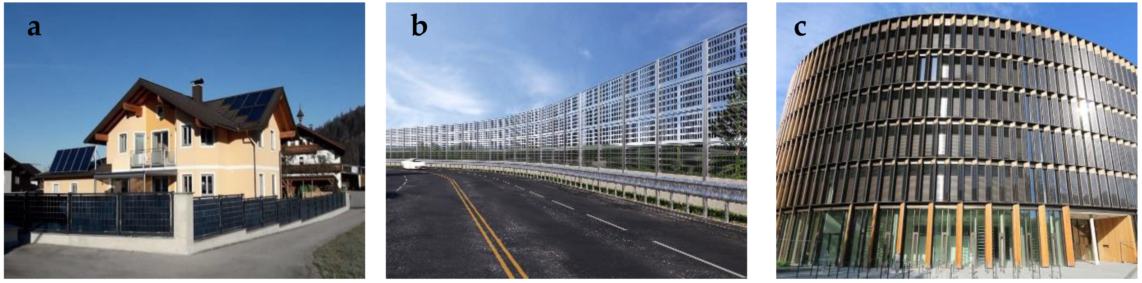
4.3. bPV Vertical Application
- as a solar fence to enclose properties and buildings and produce solar energy at the same time (Figure 15a);
- as noise barriers to reduce noise levels between noise sources and receivers (Figure 15b); and
- as a building-integrated photovoltaic (BIPV) system by integrating bPV modules into the building envelope, such as the roof or façade (Figure 15c).
5. Conclusions
Author Contributions
Funding
Data Availability Statement
Conflicts of Interest
Nomenclature
| Abbreviations | |
| bPV | Bifacial Photovoltaic |
| mono PV | Monofacial Photovoltaic |
| LCOE | Levelized Cost of Energy |
| BOS | Balance of System |
| AR | Anti-reflective |
| ARC | Antireflection Coating |
| IR | Infrared |
| PERC | Passivated Emitter Back Contact |
| PERL | Passivated Emitter Back Contact with Local Diffusion |
| PERT | Passivated Emitter Back Contact with Full Diffusion |
| HIT | Heterojunction, intrinsic thin film |
| IBC | Interdigitated Back Contact |
| DSBCSC | Double-side buried contact |
| EVA | Ethylene-Vinyl Acetate copolymer |
| C-Si | Crystalline Silicon |
| BSF | Back Surface Field |
| BG | Bifacial Gain |
| GHI | Global Horizontal Irradiance |
| AM | Air Mass |
| FF | Fill Factor |
| STC | Standard Test Conditions |
| SEM | Single Exponential Model |
| APV | Agrivoltaic |
| CPV | Concentrator Photovoltaic |
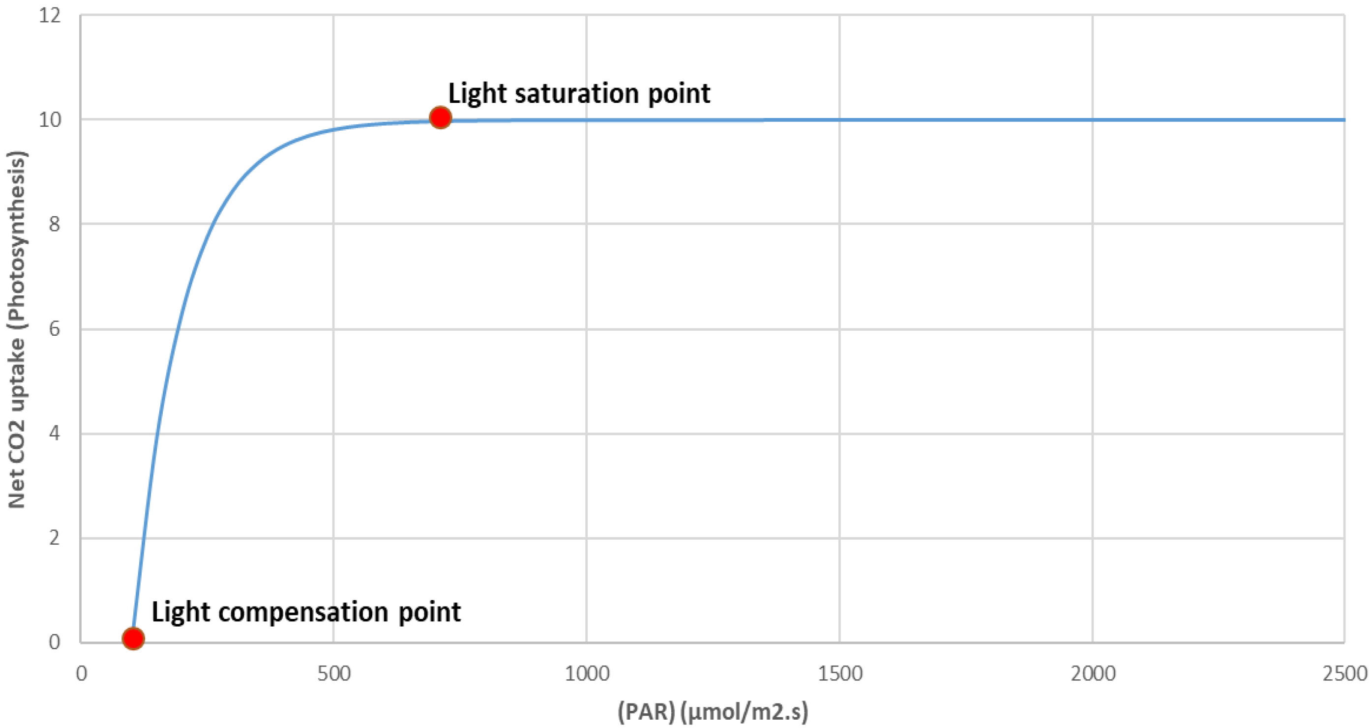
| PAR | Photosynthetically Active Radiation (μmoL m−2 s−1) |
| LCP | Light Compensation Point |
| LSP | Light Saturation Point |
| LER | Land Equivalence Ratio |
| LPF | Light Productivity Factor |
| ST | Solar Tracking |
| RT | Reverse Tracking |
| CT | Customized Tracking |
| FPV | Floating Photovoltaic |
| BIPV | Building Integrated Photovoltaic |
| Symbols | |
| Short-circuit Current Density (A/m2) | |
| Open Circuit Voltage (V) | |
| Power (W) | |
| ƞ | Power Conversion Efficiency |
| Power Conversion Efficiency for the Front/Rear in STC conditions | |
| Superscripts | |
| F and R | Front Side and Rear Side |
| Bifaciality Factor | |
| Energy Yield (KWh) | |
| Bifacial Energy Yield (KWh) | |
| Monofacial Energy Yield (KWh) | |
| Front Irradiance (W/m2) | |
| Rear Irradiance (W/m2) | |
| SR | Spectral Response (A/W) |
| Ground Albedo | |
| Spectral Reflectivity | |
| Beam Irradiance on a Horizontal Surface | |
| Ratio of Beam Radiation on the Tilted Surface to Horizontal | |
| Total Tilted Diffuse Irradiance | |
| Diffuse Horizontal Irradiance | |
| β | Photovoltaic Module Tilt Angle |
| F1 | Circumsolar Brightness Coefficient |
| F2 | Horizon Brightness Coefficient |
| Sun Zenith Angle | |
| ԑ | Sky Clearness Index |
| Δ | Brightness Index |
| L | Photovoltaic Modules Length (m) |
| h | Module-to-Ground Clearance (m) |
| Module to Sky View Factor | |
| Module to Unshaded Ground View Factor | |
| Module to Shaded Ground View Factor | |
| Total Output Power | |
| T | Temperature (K) |
| Temperature Coefficient (%/°C) | |
| Output Power at the Maximum Power Point | |
| Series Resistance | |
| Shunt Resistance | |
| Bifacial Equivalent Irradiance | |
| Band Gap Energy | |
| q | Electric Charge (1.6 × 10⁻¹⁹ C) |
| Ambient Temperature (°C) | |
| Nominal Operating Cell Temperature (°C) | |
| Irradiance under STC (1000 W/m2) | |
| ΔT | Temperature Difference (°C) |
| Module Temperature (°C) | |
| U0 | Constant Heat Transfer Coefficient (W/m2K) |
| U1 | Convective Heat Transfer Component (W/m3sK) |
| Uw | Wind Speed (m/s) |
| Specific Heat of the PV Layer | |
| Thickness of the PV Layer | |
| Density of the PV Layer | |
| Glass Transitivity (%) | |
| Lower EVA Temperature (K) | |
| Conductive Thermal Resistance Between PV Layer and Lower EVA | |
| Net Photosynthetic Rate | |
| Angle of Incidence | |
| Electrical Energy Produced by the Bifacial Modules | |
| Global Ground Irradiance (W/m2) | |
| Saturation Photosynthesis Active Radiation (μmoL m−2 s−1) | |
| Yield for a Precise Photosynthetically Active Radiation |
References
- Kreinin, L.; Bordin, N.; Karsenty, A.; Drori, A.; Eisenberg, N. Experimental Analysis of the Increases in Energy Generation of Bifacial over Mono-Facial Pv Modules. In Proceedings of the 26th European Photovoltaic Solar Energy Conference and Exhibition, Hambourg, Germany, 5–9 September 2011; pp. 3140–3143. [Google Scholar]
- Hiroshi, M. Radiation Energy Transducing Device. U.S. Patent US3278811A, 3 October 1961. [Google Scholar]
- Cuevas, A.; Luque, A.; Eguren, J.; del Alamo, J. 50 Per Cent More Output Power from an Albedo-Collecting Flat Panel Using Bifacial Solar Cells. Sol. Energy 1982, 29, 419–420. [Google Scholar] [CrossRef]
- Kasahara, N.; Yoshioka, K.; Saitoh, T. Performance Evaluation of Bifacial Photovoltaic Modules for Urban Application. In Proceedings of the 3rd World Conference on Photovoltaic Energy Conversion, Osaka, Japan, 11–18 May 2003; Volume C, pp. 2455–2458. [Google Scholar]
- Liang, T.S.; Pravettoni, M.; Deline, C.; Stein, J.S.; Kopecek, R.; Singh, J.P.; Luo, W.; Wang, Y.; Aberle, A.G.; Khoo, Y.S. A Review of Crystalline Silicon Bifacial Photovoltaic Performance Characterisation and Simulation. Energy Environ. Sci. 2019, 12, 116–148. [Google Scholar] [CrossRef]
- Kopecek, R.; Libal, J. Bifacial Photovoltaics 2021: Status, Opportunities and Challenges. Energies 2021, 14, 2076. [Google Scholar] [CrossRef]
- Dullweber, T.; Schmidt, J. Industrial Silicon Solar Cells Applying the Passivated Emitter and Rear Cell (PERC) Concept—A Review. IEEE J. Photovolt. 2016, 6, 1366–1381. [Google Scholar] [CrossRef]
- Deline, C.A.; Ayala Pelaez, S.; Marion, W.F.; Sekulic, W.R.; Woodhouse, M.A.; Stein, J. Bifacial PV System Performance: Separating Fact from Fiction; National Renewable Energy Lab.(NREL): Golden, CO, USA, 2019. [Google Scholar]
- Muehleisen, W.; Loeschnig, J.; Feichtner, M.; Burgers, A.R.R.; Bende, E.E.E.; Zamini, S.; Yerasimou, Y.; Kosel, J.; Hirschl, C.; Georghiou, G.E.E. Energy Yield Measurement of an Elevated PV System on a White Flat Roof and a Performance Comparison of Monofacial and Bifacial Modules. Renew. Energy 2021, 170, 613–619. [Google Scholar] [CrossRef]
- Rodríguez-Gallegos, C.D.; Bieri, M.; Gandhi, O.; Singh, J.P.; Reindl, T.; Panda, S.K.K. Monofacial vs Bifacial Si-Based PV Modules: Which One Is More Cost-Effective? Sol. Energy 2018, 176, 412–438. [Google Scholar] [CrossRef]
- Tina, G.M.; Bontempo Scavo, F.; Merlo, L.; Bizzarri, F. Comparative Analysis of Monofacial and Bifacial Photovoltaic Modules for Floating Power Plants. Appl. Energy 2021, 281, 116084. [Google Scholar] [CrossRef]
- Yin, H.P.P.; Zhou, Y.F.F.; Sun, S.L.L.; Tang, W.S.S.; Shan, W.; Huang, X.M.M.; Shen, X.D.D. Optical Enhanced Effects on the Electrical Performance and Energy Yield of Bifacial PV Modules. Sol. Energy 2021, 217, 245–252. [Google Scholar] [CrossRef]
- Hubner, A.; Aberle, A.; Hezel, R. Temperature Behavior of Monofacial and Bifacial Silicon Solar Cells. In Proceedings of the Conference Record of the Twenty Sixth IEEE Photovoltaic Specialists Conference, Anaheim, CA, USA, 29 September–3 October 1997; pp. 223–226. [Google Scholar]
- Ishikawa, S.N. World First Large Scale 1.25 MW Bifacial PV Power Plant on Snowy Area in Japan. In Proceedings of the 3rd bifi PV Workshop, Miyazaki, Japan, 29–30 September 2016. [Google Scholar]
- Reuters Events Renewables Giant Bifacial PV Plants Act as Springboard for Growth. Available online: https://analysis.newenergyupdate.com/pv-insider/giant-bifacial-pv-plants-act-springboard-growth (accessed on 18 January 2022).
- Burnham, L.; Riley, D.; Walker, B.; Pearce, J.M. Performance of Bifacial Photovoltaic Modules on a Dual-Axis Tracker in a High-Latitude, High-Albedo Environment. In Proceedings of the 2019 IEEE 46th Photovoltaic Specialists Conference (PVSC), Chicago, IL, USA, 16–21 June 2019; pp. 1320–1327. [Google Scholar]
- Liu, B.Y.H.; Jordan, R.C. The Long-Term Average Performance of Flat-Plate Solar-Energy Collectors. Sol. Energy 1963, 7, 53–74. [Google Scholar] [CrossRef]
- Duffie, J.A.; Beckman, W.A. Solar Engineering of Thermal Processes, 3rd ed.; Wiley: Hoboken, NJ, USA, 1982; Volume 3. [Google Scholar]
- Katsikogiannis, O.A.; Ziar, H.; Isabella, O. Integration of Bifacial Photovoltaics in Agrivoltaic Systems: A Synergistic Design Approach. Appl. Energy 2022, 309, 118475. [Google Scholar] [CrossRef]
- Assoa, Y.B.; Thony, P.; Messaoudi, P.; Schmitt, E.; Bizzini, O.; Gelibert, S.; Therme, D.; Rudy, J.; Chabuel, F. Study of a Building Integrated Bifacial Photovoltaic Facade. Sol. Energy 2021, 227, 497–515. [Google Scholar] [CrossRef]
- Pringle, A.M.; Handler, R.M.M.; Pearce, J.M.M. Aquavoltaics: Synergies for Dual Use of Water Area for Solar Photovoltaic Electricity Generation and Aquaculture. Renew. Sustain. Energy Rev. 2017, 80, 572–584. [Google Scholar] [CrossRef] [Green Version]
- Gu, W.; Ma, T.; Song, A.; Li, M.; Shen, L. Mathematical Modelling and Performance Evaluation of a Hybrid Photovoltaic-Thermoelectric System. Energy Convers. Manag. 2019, 198, 111800. [Google Scholar] [CrossRef]
- Raina, G.; Sinha, S. A Simulation Study to Evaluate and Compare Monofacial Vs Bifacial PERC PV Cells and the Effect of Albedo on Bifacial Performance. Mater. Today Proc. 2020, 46, 5242–5247. [Google Scholar] [CrossRef]
- Wang, A.; Xuan, Y. A Detailed Study on Loss Processes in Solar Cells. Energy 2018, 144, 490–500. [Google Scholar] [CrossRef]
- Chantana, J.; Horio, Y.; Kawano, Y.; Hishikawa, Y.; Minemoto, T. Spectral Mismatch Correction Factor for Precise Outdoor Performance Evaluation and Description of Performance Degradation of Different-Type Photovoltaic Modules. Sol. Energy 2019, 181, 169–177. [Google Scholar] [CrossRef]
- Dupré, O.; Vaillon, R.; Green, M.A. A Full Thermal Model for Photovoltaic Devices. Sol. Energy 2016, 140, 73–82. [Google Scholar] [CrossRef]
- Dupré, O. Physics of the Thermal Behavior of Photovoltaic Devices; INSA de Lyon: Villeurbanne, France, 2015. [Google Scholar]
- Tang, H.B.B.; Ma, S.; Lv, Y.; Li, Z.P.P.; Shen, W.Z.Z. Optimization of Rear Surface Roughness and Metal Grid Design in Industrial Bifacial PERC Solar Cells. Sol. Energy Mater. Sol. Cells 2020, 216, 110712. [Google Scholar] [CrossRef]
- Rabanal-Arabach, J.; Schneider, A. Anti-Reflective Coated Glass and Its Impact on Bifacial Modules’ Temperature in Desert Locations. Energy Procedia 2016, 92, 590–599. [Google Scholar] [CrossRef] [Green Version]
- Saive, R.; Russell, T.C.R.R.; Atwater, H.A. Enhancing the Power Output of Bifacial Solar Modules by Applying Effectively Transparent Contacts (ETCs) With Light Trapping. IEEE J. Photovolt. 2018, 8, 1183–1189. [Google Scholar] [CrossRef]
- Sepeai, S.; Sulaiman, M.Y.; Sopian, K.; Zaidi, S.H. Investigation of Back Surface Fields Effect on Bifacial Solar Cells. In AIP Conference Proceedings; American Institute of Physics: College Park, MD, USA, 2012; Volume 1502, pp. 322–335. [Google Scholar]
- Moehlecke, A.; Zanesco, I.; Luque, A. Practical High Efficiency Bifacial Solar Cells. In Proceedings of the 1994 IEEE 1st World Conference on Photovoltaic Energy Conversion—WCPEC (A Joint Conference of PVSC, PVSEC and PSEC), Waikoloa, HI, USA, 5–9 December 1994; Volume 2, pp. 1663–1666. [Google Scholar]
- Shoukry, I.; Libal, J.; Kopecek, R.; Wefringhaus, E.; Werner, J. Modelling of Bifacial Gain for Stand-Alone and in-Field Installed Bifacial PV Modules. Energy Procedia 2016, 92, 600–608. [Google Scholar] [CrossRef] [Green Version]
- Stein, J.S.; Reise, C.; Castro, J.B.; Friesen, G.; Maugeri, G.G.; Urrejola, E.E.; Ranta, S. Bifacial Photovoltaic Modules and Systems: Experience and Results from International Research and Pilot Applications; Sandia National Lab.(SNL-NM): Albuquerque, NM, USA; Livermore, CA, USA, 2021. [Google Scholar]
- Spectral Response. In Encyclopedia of Microfluidics and Nanofluidics; Springer: Boston, MA, USA, 2008; p. 1881.
- Gostein, M.; Marion, B.; Stueve, B. Spectral Effects in Albedo and Rearside Irradiance Measurement for Bifacial Performance Estimation. In Proceedings of the 2020 47th IEEE Photovoltaic Specialists Conference (PVSC), Calgary, AB, Canada, 15 June–21 August 2020; Volume 2020-June, pp. 515–519. [Google Scholar]
- Brennan, M.P.P.; Abramase, A.L.L.; Andrews, R.W.W.; Pearce, J.M.M. Effects of Spectral Albedo on Solar Photovoltaic Devices. Sol. Energy Mater. Sol. Cells 2014, 124, 111–116. [Google Scholar] [CrossRef] [Green Version]
- Myers, D.R.; Gueymard, C.A. Description and Availability of the SMARTS Spectral Model for Photovoltaic Applications. In Organic Photovoltaics V; Kafafi, Z.H., Lane, P.A., Eds.; SPIE: Bellingham, WA, USA, 2004; Volume 5520, p. 56. [Google Scholar]
- Khoo, Y.S.; Nobre, A.; Malhotra, R.; Yang, D.; Ruther, R.; Reindl, T.; Aberle, A.G. Optimal Orientation and Tilt Angle for Maximizing In-Plane Solar Irradiation for PV Applications in Singapore. IEEE J. Photovolt. 2014, 4, 647–653. [Google Scholar] [CrossRef]
- Liu, B.; Jordan, R. Daily Insolation on Surfaces Tilted towards Equator. ASHRAE J. 1961, 10, 53–59. [Google Scholar]
- Temps, R.C.; Coulson, K.L.L. Solar Radiation Incident upon Slopes of Different Orientations. Sol. Energy 1977, 19, 179–184. [Google Scholar] [CrossRef]
- Perez, R.; Seals, R.; Ineichen, P.; Stewart, R.; Menicucci, D. A New Simplified Version of the Perez Diffuse Irradiance Model for Tilted Surfaces. Sol. Energy 1987, 39, 221–231. [Google Scholar] [CrossRef] [Green Version]
- Iqbal, M. An Introduction to Solar Radiation; Elsevier: Amsterdam, The Netherlands, 1983; ISBN 9780123737502. [Google Scholar]
- Gueymard, C.A.; Lara-Fanego, V.; Sengupta, M.; Xie, Y. Surface Albedo and Reflectance: Review of Definitions, Angular and Spectral Effects, and Intercomparison of Major Data Sources in Support of Advanced Solar Irradiance Modeling over the Americas. Sol. Energy 2019, 182, 194–212. [Google Scholar] [CrossRef]
- Sandia National Laboratories. POA Ground Reflected. Available online: https://pvpmc.sandia.gov/modeling-steps/1-weather-design-inputs/plane-of-array-poa-irradiance/calculating-poa-irradiance/poa-ground-reflected/ (accessed on 1 November 2022).
- Suri, T.C.M. SOLARGIS. Available online: https://solargis.com/ (accessed on 1 November 2022).
- Meteotest Switzerland Meteonorm Software 7. Available online: http://www.meteonorm.com/ (accessed on 1 November 2022).
- PVGIS Photovoltaic Geographical Information System. Available online: http://re.jrc.ec.europa.eu/pvg_download/map_index.html%0Ahttps://re.jrc.ec.europa.eu/pvg_tools/en/%0Ahttps://re.jrc.ec.europa.eu/pvg_tools/es/#PVP%0Ahttps://ec.europa.eu/jrc/en/pvgis (accessed on 1 November 2022).
- Appelbaum, J. The Role of View Factors in Solar Photovoltaic Fields. Renew. Sustain. Energy Rev. 2018, 81, 161–171. [Google Scholar] [CrossRef]
- PV Performance Modeling Collaborative|Ray Tracing Models for Backside Irradiance. Available online: https://pvpmc.sandia.gov/pv-research/bifacial-pv-project/bifacial-pv-performance-models/ray-tracing-models-for-backside-irradiance/ (accessed on 1 November 2022).
- Radiance Software. Available online: https://floyd.lbl.gov/radiance/framed.html (accessed on 28 March 2022).
- Trace PRO Software. Available online: https://lambdares.com/tracepro/ (accessed on 28 March 2022).
- Comsol Software. Available online: https://www.comsol.com/ray-optics-module (accessed on 28 March 2022).
- Libal, J.; Kopecek, R. Bifacial Photovoltaics: Technology, Applications and Economics; Libal, J., Kopecek, R., Eds.; Institution of Engineering and Technology: Stevenage, UK, 2018; ISBN 9781785612749. [Google Scholar]
- Pelaez, S.A.; Deline, C.; MacAlpine, S.M.; Marion, B.; Stein, J.S.; Kostuk, R.K. Comparison of Bifacial Solar Irradiance Model Predictions With Field Validation. IEEE J. Photovolt. 2019, 9, 82–88. [Google Scholar] [CrossRef]
- Castillo-Aguilella, J.E.; Hauser, P.S. Bifacial Photovoltaic Module Best-Fit Annual Energy Yield Model with Azimuthal Correction. In Proceedings of the IEEE 44th Photovoltaic Specialists Conference (PVSC 2017), Washington, DC, USA, 25–30 June 2017; pp. 195–197. [Google Scholar]
- Gu, W.; Ma, T.; Ahmed, S.; Zhang, Y.; Peng, J. A Comprehensive Review and Outlook of Bifacial Photovoltaic (BPV) Technology. Energy Convers. Manag. 2020, 223, 113283. [Google Scholar] [CrossRef]
- Tossa, A.K.; Soro, Y.M.M.; Azoumah, Y.; Yamegueu, D. A New Approach to Estimate the Performance and Energy Productivity of Photovoltaic Modules in Real Operating Conditions. Sol. Energy 2014, 110, 543–560. [Google Scholar] [CrossRef]
- Ma, J.; Man, K.L.; Ting, T.O.; Zhang, N.; Guan, S.-U.U.; Wong, P.W.H.H. Approximate Single-Diode Photovoltaic Model for Efficient I–V Characteristics Estimation. Sci. World J. 2013, 2013, 1–7. [Google Scholar] [CrossRef] [Green Version]
- Ross, R.G., Jr. Design Tech for FP PV Arrays. 1981. Available online: https://www2.jpl.nasa.gov/adv_tech/photovol/ppr_81-85/Design%20Tech%20for%20FP%20PV%20Arrays_PVSC1981.pdf (accessed on 1 November 2022).
- Leonardi, M.; Corso, R.; Milazzo, R.G.; Connelli, C.; Foti, M.; Gerardi, C.; Bizzarri, F.; Privitera, S.M.S.S.; Lombardo, S.A. The Effects of Module Temperature on the Energy Yield of Bifacial Photovoltaics: Data and Model. Energies 2021, 15, 22. [Google Scholar] [CrossRef]
- Hassanian, R.; Riedel, M.; Yeganeh, N. A Review in Context to Wind Effect on NOCT Model for Photovoltaic Panel. Crimson Publ. Wings to Res. 2022, 2, 1–3. [Google Scholar]
- King, D.L.; Boyson, W.E.; Kratochvil, J.A.; Boyson, W.E.; King, D.L. Photovoltaic Array Performance Model; Sandia National Laboratories (SNL): Albuquerque, NM, USA; Livermore, CA, USA, 2004; Volume 8. [Google Scholar]
- PVPerformance Sandia Module Temperature Model. Available online: https://pvpmc.sandia.gov/modeling-steps/2-dc-module-iv/module-temperature/sandia-module-temperature-model/ (accessed on 23 May 2022).
- Faiman, D. Assessing the Outdoor Operating Temperature of Photovoltaic Modules. Prog. Photovolt. Res. Appl. 2008, 16, 307–315. [Google Scholar] [CrossRef]
- Gu, W.; Ma, T.; Li, M.; Shen, L.; Zhang, Y. A Coupled Optical-Electrical-Thermal Model of the Bifacial Photovoltaic Module. Appl. Energy 2020, 258, 114075. [Google Scholar] [CrossRef]
- Tina, G.M.; Scavo, F.B.; Gagliano, A. Multilayer Thermal Model for Evaluating the Performances of Monofacial and Bifacial Photovoltaic Modules. IEEE J. Photovolt. 2020, 10, 1035–1043. [Google Scholar] [CrossRef]
- Barron-Gafford, G.A.; Pavao-Zuckerman, M.A.; Minor, R.L.; Sutter, L.F.; Barnett-Moreno, I.; Blackett, D.T.; Thompson, M.; Dimond, K.; Gerlak, A.K.; Nabhan, G.P.; et al. Agrivoltaics Provide Mutual Benefits across the Food–Energy–Water Nexus in Drylands. Nat. Sustain. 2019, 2, 848–855. [Google Scholar] [CrossRef]
- Dupraz, C.; Marrou, H.; Talbot, G.; Dufour, L.; Nogier, A.; Ferard, Y. Combining Solar Photovoltaic Panels and Food Crops for Optimising Land Use: Towards New Agrivoltaic Schemes. Renew. Energy 2011, 36, 2725–2732. [Google Scholar] [CrossRef]
- Sato, D.; Yamada, N. Design and Testing of Highly Transparent Concentrator Photovoltaic Modules for Efficient Dual-land-use Applications. Energy Sci. Eng. 2020, 8, 779–788. [Google Scholar] [CrossRef] [Green Version]
- Domínguez, C.; Jost, N.; Askins, S.; Victoria, M.; Antón, I. A Review of the Promises and Challenges of Micro-Concentrator Photovoltaics. In AIP Conference Proceedings; AIP Publishing LLC: Melville, NY, USA, 2017; Volume 1881, p. 080003. [Google Scholar]
- Thompson, E.P.; Bombelli, E.L.; Shubham, S.; Watson, H.; Everard, A.; D’Ardes, V.; Schievano, A.; Bocchi, S.; Zand, N.; Howe, C.J.; et al. Tinted Semi-Transparent Solar Panels Allow Concurrent Production of Crops and Electricity on the Same Cropland. Adv. Energy Mater. 2020, 10, 2001189. [Google Scholar] [CrossRef]
- Zhi, L.; Yano, A.; Marco, C.; Yoshioka, H.; Kita, I.; Ibaraki, Y. Shading and Electric Performance of a Prototype Greenhouse Blind System Based on Semi-Transparent Photovoltaic Technology. J. Agric. Meteorol. 2018, 74, 114–122. [Google Scholar] [CrossRef]
- Distler, A.; Brabec, C.J.; Egelhaaf, H.J. Organic Photovoltaic Modules with New World Record Efficiencies. Prog. Photovolt. Res. Appl. 2021, 29, 24–31. [Google Scholar] [CrossRef]
- Öner, İ.V. Operational Stability and Degradation of Organic Solar Cells. Period. Eng. Nat. Sci. 2017, 5. [Google Scholar] [CrossRef] [Green Version]
- Evans, J.R. Improving Photosynthesis. Plant Physiol. 2013, 162, 1780–1793. [Google Scholar] [CrossRef] [Green Version]
- Teskey, R.O.; Sheriff, D.W.; Hollinger, D.Y.; Thomas, R.B. External and Internal Factors Regulating Photosynthesis. In Resource Physiology of Conifers; Elsevier: Amsterdam, The Netherlands, 1995; pp. 105–140. ISBN 9780126528701. [Google Scholar]
- Maire, V.; Wright, I.J.; Prentice, I.C.; Batjes, N.H.; Bhaskar, R.; van Bodegom, P.M.; Cornwell, W.K.; Ellsworth, D.; Niinemets, Ü.; Ordonez, A.; et al. Global Effects of Soil and Climate on Leaf Photosynthetic Traits and Rates. Glob. Ecol. Biogeogr. 2015, 24, 706–717. [Google Scholar] [CrossRef]
- LEACH, J.E. Some Effects of Air Temperature and Humidity on Crop and Leaf Photosynthesis, Transpiration and Resistance to Gas Transfer. Ann. Appl. Biol. 1979, 92, 287–297. [Google Scholar] [CrossRef]
- Kuo, J.; den Hartog, C. Seagrass Taxonomy and Identification Key. In Global Seagrass Research Methods; Elsevier: Amsterdam, The Netherlands, 2001; pp. 31–58. [Google Scholar]
- Runkle, B.E. Interactions of Light, CO2 and Temperature on Photosynthesis; GNP; Michigan State University: East Lansing, MI, USA, 2015; Volume 2015. [Google Scholar]
- Hartzell, S.; Bartlett, M.S.; Porporato, A. Unified Representation of the C3, C4, and CAM Photosynthetic Pathways with the Photo3 Model. Ecol. Modell. 2018, 384, 173–187. [Google Scholar] [CrossRef] [Green Version]
- Yin, X.; Struik, P.C.C. C 3 and C 4 Photosynthesis Models: An Overview from the Perspective of Crop Modelling. NJAS Wagening. J. Life Sci. 2009, 57, 27–38. [Google Scholar] [CrossRef] [Green Version]
- Mahendra, S.; Ogren, W.L.; Widholm, J.M. Photosynthetic Characteristics of Several C3 and C4 Plant Species Grown Under Different Light Intensities 1. Crop Sci. 1974, 14, 563–566. [Google Scholar] [CrossRef]
- Weselek, A.; Bauerle, A.; Hartung, J.; Zikeli, S.; Lewandowski, I.; Högy, P. Agrivoltaic System Impacts on Microclimate and Yield of Different Crops within an Organic Crop Rotation in a Temperate Climate. Agron. Sustain. Dev. 2021, 41, 59. [Google Scholar] [CrossRef]
- Marrou, H.; Guilioni, L.; Dufour, L.; Dupraz, C.; Wery, J. Microclimate under Agrivoltaic Systems: Is Crop Growth Rate Affected in the Partial Shade of Solar Panels? Agric. For. Meteorol. 2013, 177, 117–132. [Google Scholar] [CrossRef]
- Marrou, H.; Dufour, L.; Wery, J. How Does a Shelter of Solar Panels Influence Water Flows in a Soil–Crop System? Eur. J. Agron. 2013, 50, 38–51. [Google Scholar] [CrossRef]
- Othman, N.F.; Ya’acob, M.E.; Abdul-Rahim, A.S.; Hizam, H.; Farid, M.M.; Abd Aziz, S. Inculcating Herbal Plots as Effective Cooling Mechanism in Urban Planning. Acta Hortic. 2017, 1152, 235–242. [Google Scholar] [CrossRef]
- Patel, B.; Gami, B.; Baria, V.; Patel, A.; Patel, P. Co-Generation of Solar Electricity and Agriculture Produce by Photovoltaic and Photosynthesis—Dual Model by Abellon, India. J. Sol. Energy Eng. 2019, 141, 1–9. [Google Scholar] [CrossRef]
- NREL Benefits of Agrivoltaics Across the Food-Energy-Water Nexus. Available online: https://www.nrel.gov/news/program/2019/benefits-of-agrivoltaics-across-the-food-energy-water-nexus.html (accessed on 9 June 2022).
- Al-Saidi, M.; Lahham, N. Solar Energy Farming as a Development Innovation for Vulnerable Water Basins. Dev. Pract. 2019, 29, 619–634. [Google Scholar] [CrossRef] [Green Version]
- Imran, H.; Riaz, M.H. Investigating the Potential of East/West Vertical Bifacial Photovoltaic Farm for Agrivoltaic Systems. J. Renew. Sustain. Energy 2021, 13, 033502. [Google Scholar] [CrossRef]
- Sekiyama, T.; Nagashima, A. Solar Sharing for Both Food and Clean Energy Production: Performance of Agrivoltaic Systems for Corn, A Typical Shade-Intolerant Crop. Environments 2019, 6, 65. [Google Scholar] [CrossRef] [Green Version]
- Lytle, W.; Meyer, T.K.; Tanikella, N.G.; Burnham, L.; Engel, J.; Schelly, C.; Pearce, J.M. Conceptual Design and Rationale for a New Agrivoltaics Concept: Pasture-Raised Rabbits and Solar Farming. J. Clean. Prod. 2021, 282, 124476. [Google Scholar] [CrossRef]
- Tahir, Z.; Butt, N.Z. Implications of Spatial-Temporal Shading in Agrivoltaics under Fixed Tilt & Tracking Bifacial Photovoltaic Panels. Renew. Energy 2022, 190, 167–176. [Google Scholar] [CrossRef]
- Riaz, M.H.; Imran, H.; Alam, H.; Alam, M.A.; Butt, N.Z.; Ashraful, M. Crop-Specific Optimization of Bifacial PV Arrays for Agrivoltaic Food-Energy Production: The Light-Productivity-Factor Approach. IEEE J. Photovolt. 2022, 12, 572–580. [Google Scholar] [CrossRef]
- Campana, P.E.; Stridh, B.; Amaducci, S.; Colauzzi, M. Optimisation of Vertically Mounted Agrivoltaic Systems. J. Clean. Prod. 2021, 325, 129091. [Google Scholar] [CrossRef]
- Weselek, A.; Ehmann, A.; Zikeli, S.; Lewandowski, I.; Schindele, S.; Högy, P. Agrophotovoltaic Systems: Applications, Challenges, and Opportunities. A Review. Agron. Sustain. Dev. 2019, 39, 35. [Google Scholar] [CrossRef]
- Dinesh, H.; Pearce, J.M. The Potential of Agrivoltaic Systems. Renew. Sustain. Energy Rev. 2016, 54, 299–308. [Google Scholar] [CrossRef] [Green Version]
- Imran, H.; Riaz, M.H.; Butt, N.Z. Optimization of Single-Axis Tracking of Photovoltaic Modules for Agrivoltaic Systems. In Proceedings of the 2020 47th IEEE Photovoltaic Specialists Conference (PVSC), Calgary, AB, Canada, 15 June–21 August 2020; Volume 2020-June, pp. 1353–1356. [Google Scholar]
- Ullah, A.; Imran, H.; Maqsood, Z.; Butt, N.Z. Investigation of Optimal Tilt Angles and Effects of Soiling on PV Energy Production in Pakistan. Renew. Energy 2019, 139, 830–843. [Google Scholar] [CrossRef]
- Asgharzadeh, A.; Lubenow, T.; Sink, J.; Marion, B.; Deline, C.; Hansen, C.; Stein, J.; Toor, F. Analysis of the Impact of Installation Parameters and System Size on Bifacial Gain and Energy Yield of PV Systems. In Proceedings of the 2017 IEEE 44th Photovoltaic Specialist Conference (PVSC), Washington, DC, USA, 25–30 June 2017; pp. 3333–3338. [Google Scholar]
- Riaz, M.H.; Younas, R.; Imran, H.; Alam, M.A.; Butt, N.Z.; Younas, R.; Alam, M.A.; Butt, N.Z. Module Technology for Agrivoltaics: Vertical Bifacial Versus Tilted Monofacial Farms. IEEE J. Photovolt. 2021, 11, 469–477. [Google Scholar] [CrossRef]
- Riaz, M.H.; Imran, H.; Younas, R.; Butt, N.Z. The Optimization of Vertical Bifacial Photovoltaic Farms for Efficient Agrivoltaic Systems. Sol. Energy 2021, 230, 1004–1012. [Google Scholar] [CrossRef]
- Riaz, M.H.; Imran, H.; Butt, N.Z. Optimization of PV Array Density for Fixed Tilt Bifacial Solar Panels for Efficient Agrivoltaic Systems. In Proceedings of the 2020 47th IEEE Photovoltaic Specialists Conference (PVSC), Calgary, AB, Canada, 15 June–21 August 2020; Volume 2020-June, pp. 1349–1352. [Google Scholar]
- Hassanpour Adeh, E.; Selker, J.S.; Higgins, C.W. Remarkable Agrivoltaic Influence on Soil Moisture, Micrometeorology and Water-Use Efficiency. PLoS ONE 2018, 13, e0203256. [Google Scholar] [CrossRef] [Green Version]
- Next2Sun Agrivoltaics. Available online: https://www.next2sun.de/en/references/ (accessed on 22 June 2022).
- Brohm, R.; Khanh, N.Q. Dual Use Approaches for Solar Energy and Food Production—International Experience and Potentials for Vietnam; Green Innovation and Development Centre (GreenID): Hanoi, Vietnam, 2018. [Google Scholar]
- BELLINI, E. Agrivoltaics for Pear Orchards. Available online: https://www.pv-magazine.com/2020/10/02/agrivoltaics-for-pear-orchards/ (accessed on 22 June 2022).
- Beshilas, L. Floating Solar Photovoltaics Could Make a Big Splash in the USA. Available online: https://www.nrel.gov/state-local-tribal/blog/posts/floating-solar-photovoltaics-could-make-a-big-splash-in-the-usa.html#:~:text=A floating solar photovoltaic(FPV,land or on building rooftops (accessed on 5 July 2022).
- Sharma, P.; Muni, B.; Sen, D. Design Parameters of 10 KW Floating Solar Power Plant Conference. Int. Adv. Res. J. Sci. Eng. Technol. 2016, 2, 85–89. [Google Scholar] [CrossRef]
- Rodrigues, I.S.; Ramalho, G.L.B.; Medeiros, P.H.A. Potential of Floating Photovoltaic Plant in a Tropical Reservoir in Brazil. J. Environ. Plan. Manag. 2020, 63, 2334–2356. [Google Scholar] [CrossRef]
- Sahu, A.; Yadav, N.; Sudhakar, K. Floating Photovoltaic Power Plant: A Review. Renew. Sustain. Energy Rev. 2016, 66, 815–824. [Google Scholar] [CrossRef]
- Ponce, V.M.; Lohani, A.K.; Huston, P.T. Surface Albedo and Water Resources: Hydroclimatological Impact of Human Activities. J. Hydrol. Eng. 1997, 2, 197–203. [Google Scholar] [CrossRef]
- Ziar, H.; Prudon, B.; Lin, F.Y.; Roeffen, B.; Heijkoop, D.; Stark, T.; Teurlincx, S.; Senerpont Domis, L.; Goma, E.G.; Extebarria, J.G.; et al. Innovative Floating Bifacial Photovoltaic Solutions for Inland Water Areas. Prog. Photovolt. Res. Appl. 2021, 29, 725–743. [Google Scholar] [CrossRef]
- Widayat, A.A.; Ma’arif, S.; Syahindra, K.D.; Fauzi, A.F.; Setiawan, E.A.; Adhi Setiawan, E. Comparison and Optimization of Floating Bifacial and Monofacial Solar PV System in a Tropical Region. In Proceedings of the 2020 9th International Conference on Power Science and Engineering (ICPSE), London, UK, 23–25 October 2020; pp. 66–70. [Google Scholar]
- First Floating Solar Farm in Thailand with UBE. Available online: https://www.baywa-re.es/en/company/news/details/first-floating-solar-farm-in-thailand-with-ube (accessed on 12 July 2022).
- SEAC Solar Noise Barriers. Available online: https://www.mitrex.com/noise-barriers/ (accessed on 12 July 2022).
- Building-Integrated PV. Available online: https://a2-solar.com/en/building-integrated-pv/ (accessed on 12 July 2022).
- Joge, T.; Araki, I.; Takaku, K.; Nakahara, H.; Eguchi, Y.; Tomita, T. Advanced Applications of Bifacial Solar Modelus. In Proceedings of the 3rd World Conference on Photovoltaic Energy Conversion, Osaka, Japan, 11–18 May 2003; Volume C, pp. 2451–2454. [Google Scholar]
- Araki, I.; Tatsunokuchi, M.; Nakahara, H.; Tomita, T. Bifacial PV System in Aichi Airport-Site Demonstrative Research Plant for New Energy Power Generation. Sol. Energy Mater. Sol. Cells 2009, 93, 911–916. [Google Scholar] [CrossRef]
- Joge, T.; Eguchi, Y.; Imazu, Y.; Araki, I.; Uematsu, T.; Matsukuma, K. Applications and Field Tests of Bifacial Solar Modules. In Proceedings of the Conference Record of the Twenty-Ninth IEEE Photovoltaic Specialists Conference, New Orleans, LA, USA, 19–24 May 2002; pp. 1549–1552. [Google Scholar]
- de Jong, M.M.; van den Donker, M.N.; Verkuilen, S.; Folkerts, W. Self-Shading in Bifacial Photovoltaic Noise Barriers. In Proceedings of the 32nd European Photovoltaic Solar Energy Conference and Exhibition, Munich, Germany, 20–24 June 2016; Volume 53, pp. 2732–2734. [Google Scholar]
- Faturrochman, G.J.J.; de Jong, M.M.M.; Santbergen, R.; Folkerts, W.; Zeman, M.; Smets, A.H.M.H.M. Maximizing Annual Yield of Bifacial Photovoltaic Noise Barriers. Sol. Energy 2018, 162, 300–305. [Google Scholar] [CrossRef]
- Tina, G.M.; Scavo, F.B.; Aneli, S.; Gagliano, A. Assessment of the Electrical and Thermal Performances of Building Integrated Bifacial Photovoltaic Modules. J. Clean. Prod. 2021, 313, 127906. [Google Scholar] [CrossRef]
- Attoye, D.E.; Hassan, A. A Review on Building Integrated Photovoltaic Façade Customization Potentials. Sustainability 2017, 9, 2287. [Google Scholar] [CrossRef] [Green Version]
- Baumann, T.; Nussbaumer, H.; Klenk, M.; Dreisiebner, A.; Carigiet, F.; Baumgartner, F. Photovoltaic Systems with Vertically Mounted Bifacial PV Modules in Combination with Green Roofs. Sol. Energy 2019, 190, 139–146. [Google Scholar] [CrossRef]
- Corfield, L. Photovoltaic Noise Barriers. Available online: https://sunenergysite.eu/en/pvpowerplants/noisebarriers.php (accessed on 15 July 2022).
- Mishra, A. Delhi Metro To Install Bifacial Vertical Solar Panels. Available online: https://swarajyamag.com/infrastructure/delhi-metro-to-install-bifacial-vertical-solar-panels (accessed on 15 July 2022).


| Advantages | Disadvantages | |
|---|---|---|
| View Factors |
|
|
| Ray-Tracing |
|
|
| No | Location | Capacity | Further Information | Reference | |
|---|---|---|---|---|---|
| Solar Fence | 1 | St. Martin bei Lofer, Austria | 52.55 kWp | This solar fence serves as an enclosure for the chicken farm and for the self-consumption of energy, with a yield of 50 MWh/year. | [107] |
| 2 | Maishofen, Austria | 3.42 kWp | The solar fence serves as a housing enclosure and for self-consumption of energy, with a yield of 3500 KWh/year. | [107] | |
| Noise barriers | 4 | Switzerland, Zürich, Aurugg | 10 KWp | The first bifacial PV noise barrier in the world. | [128] |
| 5 | Delhi, India | 100 KWp | Noise barriers bifacial vertical panels for the Delhi Metro. | [129] |
Publisher’s Note: MDPI stays neutral with regard to jurisdictional claims in published maps and institutional affiliations. |
© 2022 by the authors. Licensee MDPI, Basel, Switzerland. This article is an open access article distributed under the terms and conditions of the Creative Commons Attribution (CC BY) license (https://creativecommons.org/licenses/by/4.0/).
Share and Cite
Mouhib, E.; Micheli, L.; Almonacid, F.M.; Fernández, E.F. Overview of the Fundamentals and Applications of Bifacial Photovoltaic Technology: Agrivoltaics and Aquavoltaics. Energies 2022, 15, 8777. https://doi.org/10.3390/en15238777
Mouhib E, Micheli L, Almonacid FM, Fernández EF. Overview of the Fundamentals and Applications of Bifacial Photovoltaic Technology: Agrivoltaics and Aquavoltaics. Energies. 2022; 15(23):8777. https://doi.org/10.3390/en15238777
Chicago/Turabian StyleMouhib, Elmehdi, Leonardo Micheli, Florencia M. Almonacid, and Eduardo F. Fernández. 2022. "Overview of the Fundamentals and Applications of Bifacial Photovoltaic Technology: Agrivoltaics and Aquavoltaics" Energies 15, no. 23: 8777. https://doi.org/10.3390/en15238777