Prediction of Mixing Uniformity of Hydrogen Injection inNatural Gas Pipeline Based on a Deep Learning Model

Abstract

It is economical and efficient to use existing natural gas pipelines to transport hydrogen. The fast and accurate prediction of mixing uniformity of hydrogen injection in natural gas pipelines is important for the safety of pipeline transportation and downstream end users. In this study, the computational fluid dynamics (CFD) method was used to investigate the hydrogen injection process in a T-junction natural gas pipeline. The coefficient of variation (COV) of a hydrogen concentration on a pipeline cross section was used to quantitatively characterize the mixing uniformity of hydrogen and natural gas. To quickly and accurately predict the COV, a deep neural network (DNN) model was constructed based on CFD simulation data, and the main influencing factors of the COV including flow velocity, hydrogen blending ratio, gas temperature, flow distance, and pipeline diameter ratio were taken as input nodes of the DNN model. In the model training process, the effects of various parameters on the prediction accuracy of the DNN model were studied, and an accurate DNN architecture was constructed with an average error of 4.53% for predicting the COV. The computational efficiency of the established DNN model was also at least two orders of magnitude faster than that of the CFD simulations for predicting the COV.

1. Introduction

As a green and clean energy with zero carbon emissions, hydrogen has attracted much attention in the energy industry in recent years. As the development of natural gas pipelines is mature, many countries have tried to blend a certain proportion of hydrogen in natural gas pipelines to transport the hydrogen and reduce household carbon emissions, and the mixture of hydrogen and natural gas is called hydrogen-enriched natural gas (HENG). Therefore, the large-scale use of HENG can not only effectively reduce the carbon emissions of end users, but also avoid the high cost of newly constructed hydrogen pipelines for pure hydrogen transportation [1,2,3]. Many studies have shown that when the hydrogen blending ratio (HBR) is less than 20% (volume fraction), it will not cause hydrogen failure in the pipelines or affect the use of the end devices obviously; thus, the HBR of common natural gas pipelines is usually between 5–20% [4,5,6]. However, due to the significant density difference between hydrogen and natural gas, there may be gas stratification in the mixing process. There are two main concerns of a high local hydrogen concentration caused by gas stratification: one is that it affects the gas supply stability of the end users and may cause the gas burner to backfire, and the other is that a high local hydrogen concentration in steel pipelines may cause hydrogen embrittlement, resulting in the leakage and explosion of HENG [7,8]. Therefore, it is of great significance to ensure the safe transportation and use of HENG by accurately and quickly predicting the hydrogen concentration distribution in the mixing process and putting forward measures to improve the mixing uniformity of hydrogen and natural gas.

The branch pipeline is usually used to mix the fluid of different components or different temperatures. For example, to ensure the fluctuations of calorific value of a natural gas pipe network within a reasonable range, the branch pipeline is used to mix different kinds of natural gas before it is injected into urban pipe networks [9,10,11]. Whether different kinds of natural gases are mixed uniformly is a key factor that affects the measurement accuracy and ensures the fair trade. In the nuclear power industry, the branch pipeline is usually used for the thermal mixing of fluids at different temperatures. A high-frequency temperature fluctuation can cause thermal fatigue of the pipeline materials; thus, many scholars carried out a series of research on thermal mixing using a branch pipeline [12,13,14,15].

The angle between the branch pipeline and the main pipeline has a great influence on the gas mixing process. The mixing efficiency of a T-junction pipeline (the angle between the branch pipeline and main pipeline is 90°) is usually higher than that of a Y-junction pipeline (the angle between the branch pipeline and main pipeline is smaller or larger than 90°). This is because when the velocity direction of two kinds of fluids is perpendicular, the collision and shear effects are more intense, and the mutual diffusion between the fluids is much stronger. The injection branch pipeline can be arranged at the bottom or top of the T-junction pipeline. Because the density of hydrogen is much less than that of natural gas, the buoyancy effect will force it to flow toward the top of the main pipeline. When the branch pipeline is located at the bottom of the main pipeline, the buoyance effect is more beneficial to the diffusion and mixing between hydrogen and natural gas [16].

The mixing uniformity is an important index to evaluate the mixing effect of hydrogen and natural gas in a T-junction pipeline. The most commonly used parameter to describe the mixing uniformity is the coefficient of variation (COV) of a hydrogen concentration on a pipeline cross section. The calculation accuracy of COV is closely related to the number of concentration measurement points, and more measurement points can better reflect the real mixing state of the gases. However, limited by the experimental condition, it is impossible to arrange too many concentration sensors on a pipeline cross section. In addition, too many concentration sensors can affect the gas flow state in the pipeline. To avoid this problem, Jegatheeswaran [17] adopted noninvasive electrical resistance tomography (ERT) to measure the gas concentration in the pipeline in order to calculate the COV. However, this method still has the shortcoming of a low measurement resolution. In addition to the limitation of concentration measurement methods, experimental safety is also an important issue. Because both natural gas and hydrogen are flammable and explosive gases, it is easy to cause explosions once a gas leakage occurs in indoor mixing experiments. Compared with experiments, the numerical simulation has advantages of safety and reliability, low cost, flexible variable control, etc. It has been widely used in the research of gas mixing. However, the mixing of hydrogen and natural gas in pipelines often requires a flow distance of tens or even hundreds of times the pipeline diameter length to achieve uniform mixing [18,19]; thus, the grid number of a geometric CFD model is often large, and the computational cost is high. In addition, the working conditions of different natural gas pipelines vary largely; for example, the flow rate, pipeline diameter, and gas temperature maybe quite different. The CFD method under specific conditions can only simulate the gas mixing process of a certain pipeline. Because the CFD simulation of multiple working conditions is time-consuming, it is difficult to realize the fast prediction of hydrogen mixing process in different natural gas pipelines.

The deep neural network (DNN) has been widely used in natural gas pipeline transportation technology in recent years, such as the prediction of failure pressure of defective pipelines [20,21], leak detection of buried pipelines [22,23], optimization of gas supply reliability [24], intelligent pipeline control [25], etc. To solve the problem of computational efficiency of the CFD simulation in predicting the mixing uniformity of hydrogen and natural gas under different working conditions of a natural gas pipeline, in this work, the result data obtained from the CFD simulations were collected as the sample data, and an accurate and efficient DNN model was established to quickly and accurately predict the mixing uniformity of hydrogen injection and mixing in a natural gas pipeline under different working conditions. In this study, the pipeline mixing conditions, including flow velocity, HBR, gas temperature, pipeline diameter ratio, and flow distance, were taken as the input layer nodes of the DNN, and the COV of the hydrogen concentration was taken as the output layer node. The architecture of the DNN was constructed by a reasonable selection of the hidden layer number, node number, activation function, and learning rate. It should be noted that the transportation of HENG using a pipeline is a relatively new issue, and the experimental research on the mixing mechanism of natural gas and hydrogen in the natural pipeline is still rarely reported in the literature. Thus, this paper is a preliminary work that mainly focuses on the simulation study and is not compared with the real experimental data and measurements due to a lack of relevant research within the literature.

The structure of this paper is organized as follows: in Section 2, the physical and mathematical models of hydrogen mixing in the natural gas pipeline are established; in Section 3, the numerical methods, including mesh generation and parameter settings of the CFD simulation, are briefly introduced; in Section 4, the influences of the main factors on the COV or mixing uniformity of hydrogen and natural gas are discussed; in Section 5, the DNN model is established based on the CFD simulation data, and the accuracy and efficiency for COV prediction are analyzed and compared; in Section 6, the concluding remarks of this study are summarized.

2. Physical and Mathematical Models

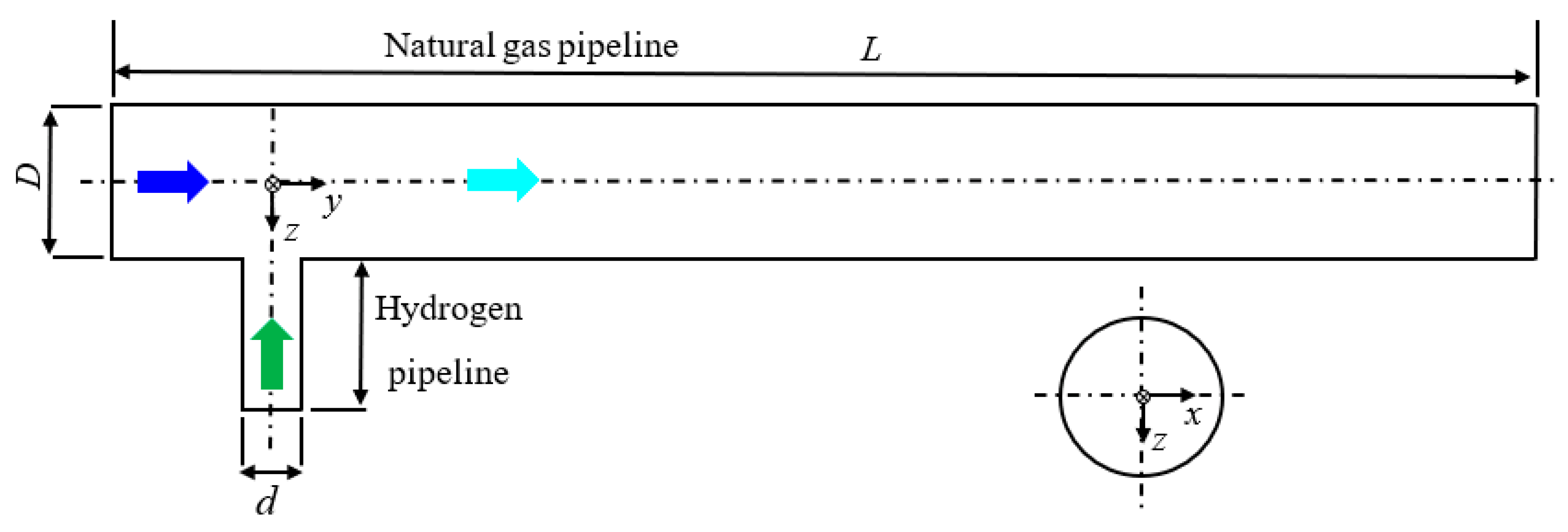
2.1. Physical Model

In this study, the hydrogen was injected into a natural gas pipeline (main pipeline) through a T-junction branch pipeline, as shown in Figure 1. The diameter of the natural gas pipeline is D; the diameter of the branch pipeline for the hydrogen injection is d, and the total length of the natural pipeline is L. The branch pipeline for the hydrogen injection was arranged at the bottom of the natural gas pipeline. The flow direction of the hydrogen was perpendicular to that of the natural gas, which can enhance the mixing of hydrogen and natural gas in a natural gas pipeline.

2.2. Mathematical Model

The composition of natural gas contains a variety of hydrocarbon and nonhydrocarbon components, among which methane is the main component. Generally, the volume fraction of methane is usually above 90%. To simplify the simulation, in this study, the natural gas was simplified as methane, and the mixing process was simplified as the mixing of hydrogen and methane.

The three-dimensional general mathematical model of the hydrogen and natural gas mixing process in the T-junction pipeline included the continuity equation, momentum equation, component transport equation, energy equation, and k-ε turbulence model, which are introduced below.

The continuity equation of the hydrogen–methane mixture reads,

$$\frac{\partial \rho }{\partial t}+\frac{\partial (\rho u_i)}{\partial x_i}=0$$

(1)

where ρ is the density of gas mixture; t is the time; u_i is the velocity component along the i direction, and i = x, y, z.

The momentum equation can be written as,

$$\frac{\partial \left(\rho u_i\right)}{\partial t}+\frac{\partial \left(\rho u_i{u}_j\right)}{\partial x_j}=-\frac{\partial p}{\partial x_i}+\frac{\partial }{\partial x_j}\left[\mu \left(\frac{\partial u_i}{\partial x_j}+\frac{\partial u_j}{\partial x_i}\right)\right]+\rho f_i$$

(2)

where p is the pressure; μ is the effective dynamic viscosity; f_i is the gravitational body force acting on the gas flow, which represents the buoyancy effect of hydrogen and methane due to the difference in density.

The mixing of hydrogen and methane is a multicomponent fluid flow process, and the mass transfer process can be described by the species transport equation,

$$\frac{\partial \left(\rho c_{\mathrm{s}}\right)}{\partial t}+\frac{\partial }{\partial x_j}\left(\rho u_j{c}_{\mathrm{s}}\right)=\frac{\partial }{\partial x_j}\left(D_{\mathrm{s}}\rho \frac{\partial c_{\mathrm{s}}}{\partial x_j}\right)$$

(3)

where c_s is the volume concentration of the gas component s; D_air-s is the diffusion coefficient of the gas component s in the air, $D_{{\mathrm{air}-\mathrm{H}}_2}=7.6\times {10}^{-5} {\mathrm{m}}^2/\mathrm{s}$ and $D_{{\mathrm{air}-\mathrm{CH}}_4}=1.6\times {10}^{-5} {\mathrm{m}}^2/\mathrm{s}$ [26].

The temperature variation of the mixing process of hydrogen and methane can be described by the following simplified energy equation:

$$\frac{\partial \left(\rho c_{p}T\right)}{\partial t}+\frac{\partial \left(\rho c_p{u}_{j}T\right)}{\partial x_j}=\frac{\partial }{\partial x_j}\left(\lambda \frac{\partial T}{\partial x_j}\right)+S$$

(4)

where T is the gas temperature; λ is the heat conductivity coefficient; c_v is the specific heat at constant volume; S is the source term.

The standard k-ε turbulence model was applied in this study to describe the turbulent state of the gas mixing process [27,28],

$$\frac{\partial }{\partial t}\left(\rho k\right)+\frac{\partial }{\partial x_i}\left(\rho u_{i}k\right)=\frac{\partial }{\partial x_j}\left[\left(\mu +\frac{{\mu }_t}{{\sigma }_k}\right)\frac{\partial k}{\partial x_j}\right]+G_K+G_b-\rho \epsilon -Y_M+S_k$$

(5)

$$\frac{\partial }{\partial t}\left(\rho \epsilon \right)+\frac{\partial }{\partial x_i}\left(\rho u_i\epsilon \right)=\frac{\partial }{\partial x_j}\left[\left(\mu +\frac{{\mu }_t}{{\sigma }_{\epsilon }}\right)\frac{\partial \epsilon }{\partial x_j}\right]+C_{1\epsilon }\frac{\epsilon }{k}\left(G_K+C_{3\epsilon }{G}_b\right)-C_{2\epsilon }\rho \frac{{\epsilon }^2}{k}+S_{\epsilon }$$

(6)

where G_k is the generation of turbulent kinetic energy due to the mean velocity gradients; G_b is the generation of turbulent kinetic energy due to buoyancy; Y_M is the contribution of fluctuating dilatation in compressible turbulence to the overall dissipation rate; the constants are $C_{1\epsilon }$ = 1.44, $C_{2\epsilon }$ = 1.92, ${\sigma }_k=1.0$, and ${\sigma }_{\epsilon }=1.3$.

3. Numerical Methods

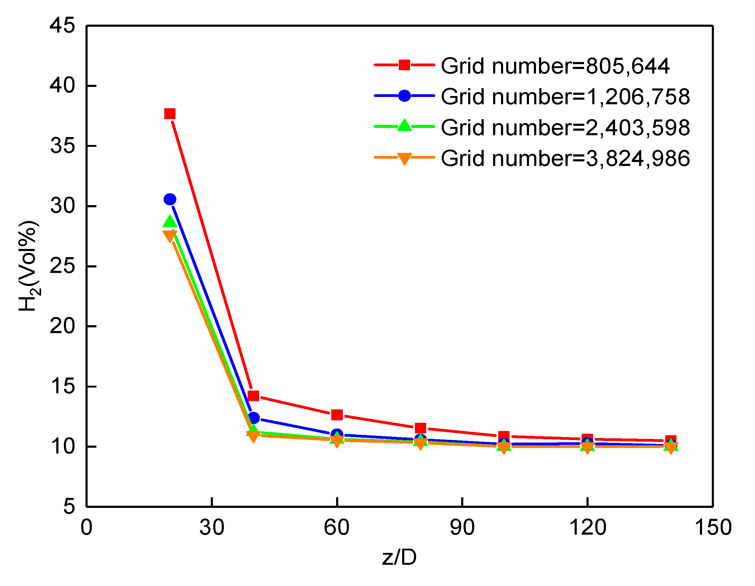
3.1. Mesh Generation

In this study, ICEM 19.2 was used to generate the mesh, and the computational domain was divided by structured grids. The overlapping part of the branch pipeline and the natural gas pipeline was connected by Interface. The mesh generation result of the computational domain is shown in Figure 2. To test the grid-independent solution, Figure 3 shows the variation of the hydrogen concentration on different pipeline cross sections along the central axis of the natural gas pipeline by using different grid numbers. When the grid number is 2,403,598, the change in hydrogen concentration is basically consistent with that by using 3,824,986 grids. Therefore, we considered that the grid-independent solution can be obtained when 2,403,598 grids were adopted; thus, the mesh generation scheme of 2,403,598 grids was used in this study.

3.2. CFD Solution Methods

In this study, the model and scheme settings for the CFD simulation by using ANSYS Fluent are shown in

Table 1. Model and discrete scheme settings.

Item	Settings in ANSYS Fluent
The turbulence model	Standard k-ε; full buoyancy effects
Near-wall treatment	Standard wall functions
Pressure–velocity coupling	SIMPLE
The spatial discretization of gradient	Least squares cell-based
The spatial discretization of pressure	Second order
The spatial discretization of momentum	Second-order upwind
The spatial discretization of energy	Second-order upwind
The spatial discretization of turbulent dissipation rate	First-order upwind
The spatial discretization of turbulent kinetic energy	First-order upwind

.

4. Analysis of Different Factors

The coefficient of variation (COV) reflects the degree of data dispersion, and it is the ratio of the standard deviation of the original data to their mean, regardless of the influence of the measurement scale and dimension. The COV has been widely used in the study of various fluid mixing [29]. In this study, the COV of the hydrogen concentration on the pipeline cross section was used to quantitatively characterize the mixing uniformity of hydrogen and natural gas, which is defined as,

$$\mathrm{COV}=\frac{1}{\overline{c}}\sqrt{\frac{{\displaystyle \sum _{i=1}^n{\left(c_i-\overline{c}\right)}^2}}{n-1}}$$

(7)

where c_i is the volume fraction of the hydrogen concentration at the sampling point; $\overline{c}$ is the average volume fraction of the hydrogen concentration at all sampling points; n is the number of sampling points, the larger the value of n, the more accurate the COV. In this study, all grid nodes on a pipeline cross section were set as sampling points. In engineering practice, hydrogen and natural gas can be considered completely mixed and uniform when the COV ≤ 0.05.

4.1. Influence of Gas Flow Velocity

In this part, the influence of the flow velocity of hydrogen and methane on the variation of the mixing uniformity of the gas mixture in the T-junction pipeline was explored. In order to control the variables for convenient discussion, the calculation parameters except the flow velocity were kept the same in the CFD simulations. In the simulation, the hydrogen blending ratio HBR was set as 10%; the pipeline pressure p was set as 0.3 MPa; the gas temperature T was set as 300 K, and the diameter ratio between the branch pipeline and the natural gas pipeline d/D was set as 0.2.

When the HBR was fixed, the ratio of the flow velocity between hydrogen and methane can be calculated by the following equation:

$$\frac{v_{{\mathrm{H}}_2}}{v_{{\mathrm{CH}}_4}}={\left(\frac{D}{d}\right)}^2\cdot \frac{\mathrm{HBR}}{1-\mathrm{HBR}}$$

(8)

where $v_{{\mathrm{H}}_2}$ is the flow velocity of hydrogen; $v_{{\mathrm{CH}}_4}$ is the flow velocity of methane; $D$ is the diameter of the natural gas pipeline; $d$ is the diameter of the branch pipeline; HBR is the hydrogen blending ratio.

Figure 4 shows the variation of the hydrogen concentration in the T-junction pipeline at the flow velocity of $v_{{\mathrm{CH}}_4}=1 \mathrm{m}/\mathrm{s}$ and $v_{{\mathrm{H}}_2}=2.78 \mathrm{m}/\mathrm{s}$. When hydrogen flows into the natural gas pipeline through the branch pipeline, the hydrogen will flow to the top of the natural gas pipeline under the effect of its original flow direction and buoyancy force, as shown in Figure 4a. At the same time, driven by the flow of methane, the hydrogen flows forward along the natural gas pipeline. As the flow progresses, the mixing of hydrogen and methane in the natural gas pipeline becomes more and more uniform. As can be seen from Figure 4b, at the pipeline cross section of z = 13 D, hydrogen and methane are basically mixed uniformly in the natural gas pipeline.

For further analysis, the hydrogen concentration at the top, bottom, and middle of the natural gas pipeline and the change of the COV along with the flow distance (different pipeline cross sections) are demonstrated in Figure 5. As the flow distance increases, the hydrogen concentration at the top of the natural gas pipeline increases and the hydrogen concentration at the bottom of the natural gas pipeline decreases, and at the middle of natural gas pipeline, it increases first and then decreases. The reason for this interesting phenomenon can be attributed to the fact that under the effect of buoyancy force, hydrogen gas flows to the top of the natural gas pipeline. Figure 5 also illustrates that the COV of the hydrogen concentration is smaller than 0.05 when z/D > 21 (21st pipeline cross section), which indicates that the hydrogen and methane have been mixed uniformly.

Figure 6 displays the change of the hydrogen concentration in the T-junction pipeline at the flow velocity $v_{{\mathrm{CH}}_4}=10 \mathrm{m}/\mathrm{s}$ and $v_{{\mathrm{H}}_2}=27.78 \mathrm{m}/\mathrm{s}$. As can be seen from Figure 6a, it is more difficult to change the velocity direction of hydrogen due to the increase in the flow velocity; thus, the hydrogen mainly accumulates at the bottom of the natural gas pipeline and slowly diffuses to the top of the natural gas pipeline. Figure 6b demonstrates that with the increase in the flow distance, the hydrogen and methane are basically mixed uniformly in the natural gas pipeline. Figure 7 presents the variation of the hydrogen concentration and the COV at different positions (cross sections) along the natural gas pipeline. When we compared Figure 7 with Figure 5, we found that in Figure 7, the hydrogen concentration and variation trend of the COV along with the flow distance were basically consistent with Figure 5 at the flow velocity of $v_{{\mathrm{CH}}_4}=1 \mathrm{m}/\mathrm{s}$ and $v_{{\mathrm{H}}_2}=2.78 \mathrm{m}/\mathrm{s}$; the main difference was that a longer flow distance was needed to achieve uniform mixing in Figure 7. Figure 7 shows that when z > 178 D and the COV ≤ 0.05 uniform mixing of hydrogen and methane has been achieved.

From the above analysis, it can be inferred that the gas flow velocity has a great influence on the mixing uniformity of hydrogen and methane in the natural gas pipeline. As the gas flow velocity increases, it becomes more difficult for the buoyancy to change the flow direction of hydrogen, which results in a longer flow distance for hydrogen and methane to fully mix. Figure 8 shows the variation of the COV under different gas flow velocities of methane at a flow distance of z = 40 D; we found that the COV was positively correlated with the gas flow velocity. When $v_{{\mathrm{CH}}_4}=1 \mathrm{m}/\mathrm{s}$ and the COV = 0.049, and it was smaller than 0.05, the hydrogen and methane were mixed uniformly. When $v_{{\mathrm{CH}}_4}=10 \mathrm{m}/\mathrm{s}$ and the COV = 0.673, the hydrogen and methane were essentially dispersed.

4.2. Influence of Gas Temperature

In this part, the influence of the pipeline transportation temperature on gas mixing is analyzed and discussed. In the CFD simulation, the gas temperature T was set between 253–313 K; the flow velocity of methane was set as $v_{{\mathrm{CH}}_4}=1 \mathrm{m}/\mathrm{s}$; the hydrogen blending ratio HBR was set as 10%; the diameter ratio between the branch pipeline and the natural gas pipeline was set as d/D = 0.2, and the pipeline pressure p was set as p = 0.3 MPa. Figure 9 shows the variation of the COV and hydrogen concentration at the flow distance of z = 40 D (40th cross section) under different gas temperatures. With the increase in gas temperature, the COV gradually decreases and the gas mixing uniformity increases. The reason is that the increase in gas temperature makes the irregular thermal motion of the molecules more violent, which enhances the molecular diffusion between hydrogen and methane and then improves the mixing uniformity.

4.3. Influence of Hydrogen Blending Ratio

The influence of the hydrogen blending ratio on the mixing uniformity of hydrogen and methane is analyzed in this part. According to the literature, when the HBR is lower than 20%, the blending of hydrogen into natural gas has tiny effects on the compatibility of the pipeline and the ignition stability of the burner. Therefore, the upper limit of the HBR was set as 20% in this study. In the CFD simulations, four groups of HBRs, 5%, 10%, 15%, and 20%, were considered, and the other calculation parameters were set as $v_{{\mathrm{CH}}_4}=1 \mathrm{m}/\mathrm{s}$, T = 300 K, d/D = 0.2, and p = 0.3 MPa. Figure 10 demonstrates the COV and distribution of the hydrogen concentration at the flow distance of z = 40 D (40th cross section) under different HBRs. The figure indicates that with the increase in HBR, the COV gradually decreases and the gas mixing tends to be more uniform.

4.4. Influence of Pipeline Diameter Ratio

In this part, the effects of the diameter ratio of the hydrogen injection branch pipeline to the main natural gas pipeline on the mixing uniformity are investigated. In the CFD simulation, the diameter ratio d/D was set as between 0.15 and 0.4, and the other calculation parameters were set as $v_{{\mathrm{CH}}_4}=1 \mathrm{m}/\mathrm{s}$, T = 300 k, HBR = 10%, and p = 0.3 MPa. Figure 11 demonstrates the COV and distribution of the hydrogen concentration at the flow distance of z = 40 D (40th cross section) under different diameter ratios d/D. As can be seen from Figure 11, with the increase in the branch pipeline diameter, the COV gradually decreases and the hydrogen and methane are mixed more uniformly. There are two main reasons for this result. First, the increase in the branch pipeline diameter enlarges the contact area between the hydrogen and methane, thus enhancing the mass transfer of the mixed gas. Second, when the HBR and flow velocity of methane are fixed, the flow velocity of hydrogen decreases with an increase in the branch pipeline diameter. Therefore, the increase in the branch pipeline diameter can improve the mixing uniformity.

5. COV Prediction Based on a Deep Neural Network Model

The mixing uniformity of hydrogen and natural gas can affect the safety of pipeline transportation and downstream end users. Through CFD simulations in Section 4, a series of qualitative analysis were carried out to reveal the influence of different factors on mixing uniformity. However, in real engineering practice, the full-scale CFD simulation is usually time-consuming and cannot meet the requirements of a quick response and fast calculation of the mixing uniformity under various working conditions. To solve this issue and predict the mixing uniformity of hydrogen and natural gas quickly and accurately in engineering practice, in this Section, a deep neural network (DNN) model is established based on the data obtained from CFD simulations.

5.1. Establishment of DNN Model

The DNN model is derived from the traditional Back Propagation (BP) neural network. A complete BP neural network includes input layer, hidden layer, and output layer, and the DNN model is a neural network model containing multiple hidden layers [30,31]. Thus, the DNN model can overcome the limitation of a traditional BP neural network by deep nonlinear network structures. The calculation process of the DNN model mainly includes two stages: forward propagation and error back propagation. For forward propagation, each node has input and output values. Except for the input and output values in the input layer, the output values of other nodes are calculated by,

$$\mathit{O}=f(\mathit{x})$$

(9)

where O is the output vector of each layer node; x is the input vector of each layer node; f is the active function, and the commonly used activation function includes Sigmoid, Tanh, Relu, LeakyRelu, Prelu, Softplus, etc. [32,33].

The input value x of each node (except the input layer) is obtained by adding the bias b to the inner product of the output value O of the node at the previous layer and the weight w of the connection between the node at the previous layer and that layer. Assuming the current node is j th node in l th layer and the node number in the previous layer l-1 is n, the input value of the current node can be written as,

$$x_j^l={\displaystyle \sum _{i=1}^n\left(w_{ij}^{l-1}{O}_i^{l-1}+b_{ij}^{l-1}\right)}$$

(10)

where w is the weight of the node connected to the upper layer; b is the bias.

In the forward propagation process, the input values of the nodes at each layer are derived from the output values of the nodes at the previous layer. Assuming that there are m hidden layers, the relationship between the input values and output values can be formulated as,

$$\mathit{O}=f_m({\mathit{w}}_m{f}_{m-1}({\mathit{w}}_{m-1}{f}_{m-2}(\dots f_1({\mathit{w}}_1{\mathit{x}}_1+{\mathit{b}}_1)\dots +{\mathit{b}}_{m-2})+{\mathit{b}}_{m-1})+{\mathit{b}}_m)$$

(11)

The error back propagation process is that when the output layer is inconsistent with the expected output, the adjustment amount of the weight w and bias b are calculated according to the error value to modify the values of w and b. The mean square deviation of the output layer can be written as,

$$Err=\frac{1}{N}{{\displaystyle \sum _{p=1}^N‖\mathit{O}-\widehat{\mathit{O}}‖}}^2$$

(12)

To iteratively adjust the weights, the gradient descent method was adopted in this work. The expression of the connection weights between l layers after m iterations is,

$${\mathit{w}}^l(m+1)={\mathit{w}}^l(m)-\alpha \frac{\partial Err}{\partial {\mathit{w}}^l}$$

(13)

where α denotes the learning rate to prevent the neural network from failing into the saturation zone when the input value of the neuron is too large. Generally, the value of α is between 0 and 1.

The calculation of the DNN model is a process of repeatedly tuning and improving weights. Unlike shallow neural networks, the number of hidden layers in the DNN model is greater than 1. To establish an accurate DNN model [34] in this study, the input layer consisted of five nodes, which were HBR, gas temperature T, ratio of flow distance to pipeline diameter z/D, flow velocity of methane v, and diameter ratio of branch pipeline to natural gas pipeline d/D. The output layer had only one node, the COV of the hydrogen concentration on the pipeline cross section that represented the mixing uniformity of hydrogen and methane. The architecture of the established DNN model for predicting COV is shown in Figure 12.

(1)

Determination of hidden layer number and node number

The selection of the appropriate hidden layer number and node number is significant for constructing an efficient and accurate DNN model. First, a series of trial calculations were carried out to train and test the DNN model under different hidden layer numbers and node numbers. Among the 1016 groups of sample data obtained from the CFD simulations in Section 4, 10 groups of data were randomly collected as the test sets, and the remaining 1006 groups of data were used as the training sets.

When the node number in one hidden layer was set as 10, the average relative error of the predicted COV compared with the 10 test sets under different hidden layer numbers is shown in Figure 13a. The relative error gradually decreased with the increase in the hidden layer number, and reached the lowest average relative error of 1.68% when the hidden layer number l = 11. Since then, the number of hidden layers continued to increase, and the average relative error fluctuated upward. Therefore, the number of hidden layers in the DNN model was selected as 11 in this study. With the hidden layer number l = 11, Figure 13b depicts the average relative error of the predicted COV compared with the 10 test sets under different node numbers and shows that the average relative error declined with the increase in node numbers. It is apparent that selecting more nodes can help to gain good prediction accuracy, but this deteriorated the prediction efficiency at the same time. In addition, a large node number may cause overfitting of the DNN model [35,36]. Because the average relative error when the node number was 40 was close to that when the node number was 50, the node number in the hidden layer was set as 40 in this study to strike a balance between prediction efficiency and overfitting.

(2)

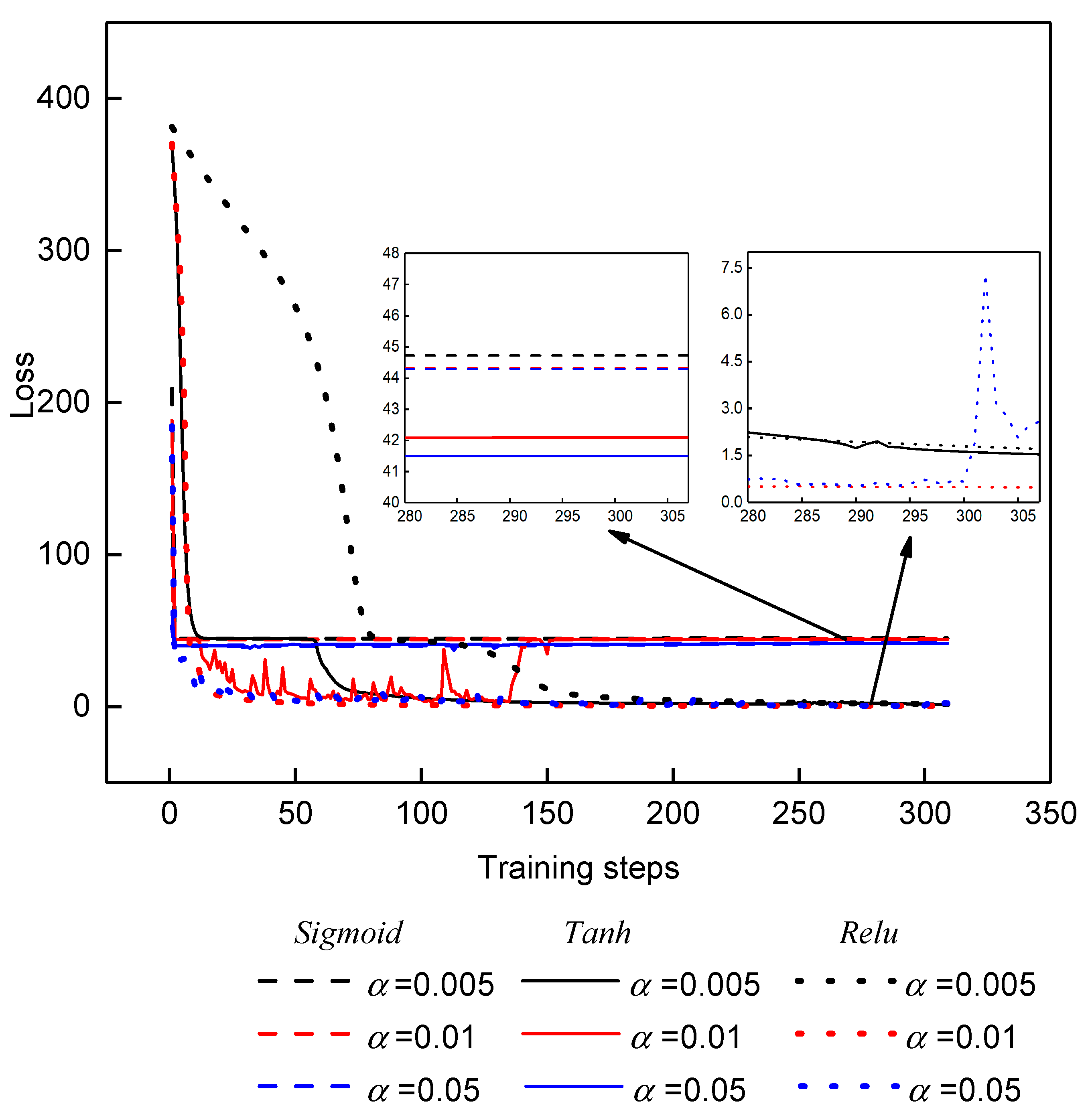
Determination of activation function and learning rate

The activation function is an important parameter in the DNN model, which can perform nonlinear mapping between input variables and output variables to improve the prediction capability of the DNN model. In this study, the iterative loss of the DNN model using three commonly used activation functions Sigmoid, Tanh, and Relu with the learning rates α = 0.005, α= 0.01, and α= 0.05 was calculated, as shown in Figure 14.

Figure 14 indicates the DNN model using the Sigmoid function and shows a phenomenon of vanishing gradient, and the iterative loss was between 44 and 45 and did not change with the increase in training number, resulting in the divergence. The reason for the vanishing gradient was mainly because of the saturation zone of the Sigmoid function, and the gradient of the inactive area tended to be 0. When the input value of the neuron node fell in this zone, if the number of hidden layers deepened, the input layer node had less and less influence on the deep node. As a result, the weight update was slow and the back-propagation process ended early with the increase in iteration. The Sigmoid function has been commonly used in traditional shallow artificial neural networks, but with the increase in the layer number, the vanishing gradient will become more serious. The Tanh function with learning rates of α = 0.01 and α = 0.05 also generated a vanishing gradient, and the calculation only converged when α = 0.005. For the vanishing gradient problem, the Tanh function performed slightly better than the Sigmoid function. The Relu function is a linear function when the input value is greater than 0, and the output is 0 when the input value is less than 0, which solves the problem of the vanishing gradient well. The iterative loss converged under the three learning rates, and the loss was the minimum value when α = 0.01; thus the Relu function was selected as the activation function and the learning rate of α = 0.01 in the DNN model.

5.2. Results and Discussion

(1)

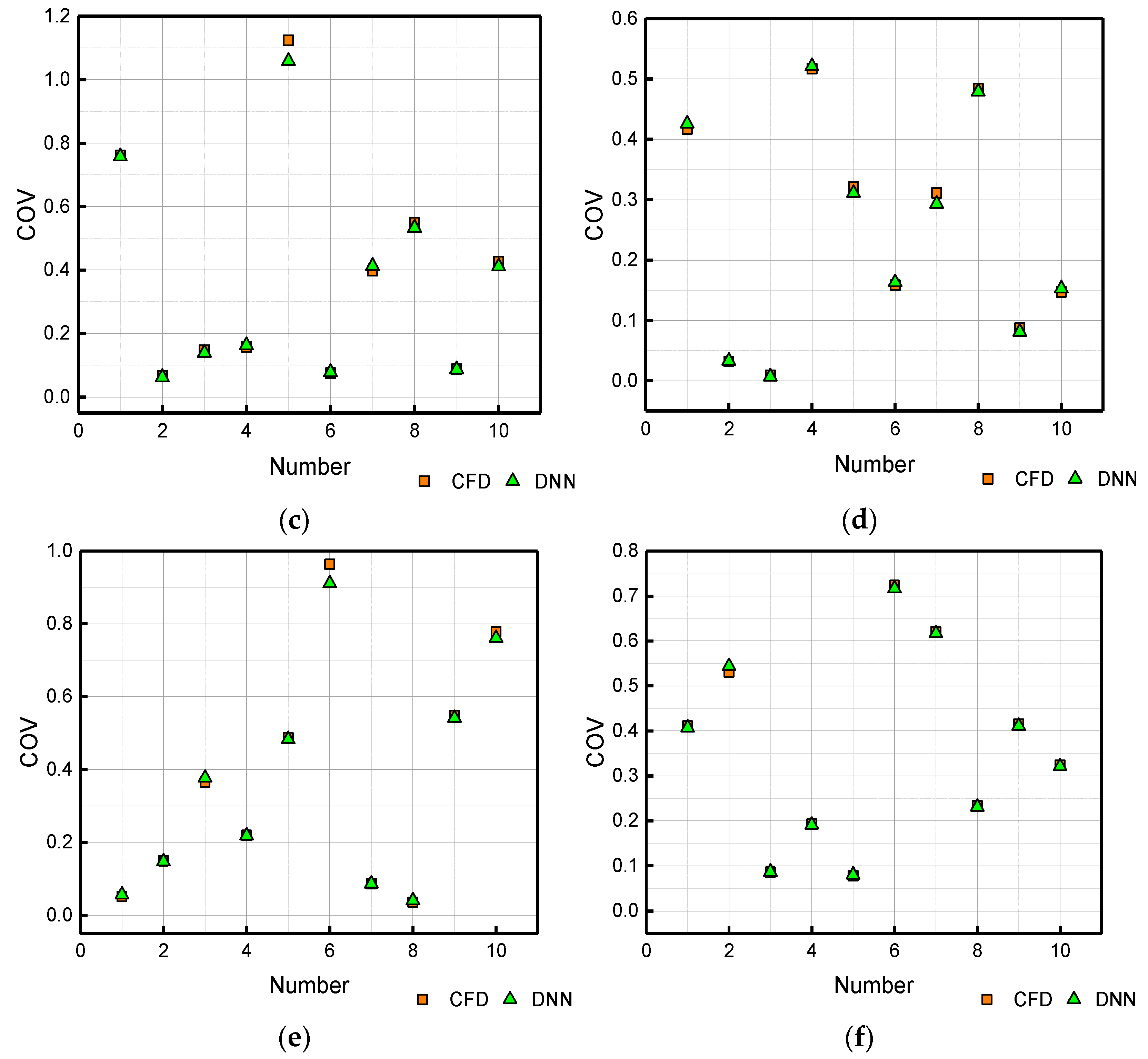
Prediction accuracy

When the hidden layer number, node number, activation function, and learning rate were determined, the architecture of the DNN model was constructed. Then, the DNN model was trained to improve the perdition performance. Each training set and test set were randomly selected from the total sample set, and 10 groups of data were selected as the test sets, and the remaining 1006 groups of data were the training sets. To ensure that the extracted test sets were representative, there was a total of six random data extractions, and six test sets including 10 groups of data were generated.

Figure 15 shows the comparison of the predicted COV by the DNN model and the COV from six randomly selected test sets calculated by CFD simulations. The predicted COV and the COV by CFD simulations agree well with each other. The comparison indicates that the average error between the DNN-predicted COV and the COV from six randomly selected test sets is 5.05%, 5.68%, 3.65%, 7.46%, 3.85%, and 1.29%, and the overall average error is only 4.53%. The comparison results illustrate that the proposed DNN model is capable of accurately predicting the COV of mixing uniformity.

(2)

Comparison of computational efficiency

To compare the computational efficiency of the DNN model and the CFD simulations,

Table 2. CPU time cost of CFD simulations.

No.	Grid Number	CPU Time (s)
1	2,403,598	18,654
2	2,403,598	18,570
3	2,403,598	19,245
4	2,205,874	16,357
5	2,804,592	20,548
6	2,804,592	21,576
7	2,403,598	19,354
8	2,584,256	18,946
Total		153,250 (1.73 day)

presents the CPU time cost for the CFD simulations of eight groups of data, and

Table 3. Comparison of CPU time cost.

Method	CPU Time (s)	Acceleration
CFD	153,250	1
DNN (offline + online)	351 + 0.01	436
DNN (online)	=0.01	=1.5 × 107

shows the comparison of the CPU time cost between the DNN model and the CFD simulations. It should be noted that in Table 3, the “offline + online” calculation using the DNN model includes the training process and prediction process, but the online calculation using the DNN model only refers to the prediction process.

Table 2 indicates that the total CPU time cost for the CFD simulations of eight groups of COV is 153,250 s, while Table 3 shows that the CPU time consumption for the DNN model to predict eight groups of the COV is only 0.01 s. From this perspective, the DNN model can accelerate the calculation by 1.5 × 10⁷ times compared with the CFD simulations. However, it is worth noting that the main time consumption of the DNN model lies in the offline training process. For the established 11-layer, 40-node DNN model in this study, the training time was approximately 351 s. Therefore, the computational efficiency of the DNN model was still 436 times higher than that of the CFD simulations, even considering the CPU time cost of the offline training time in the DNN model. However, compared with the CFD simulations, the acceleration of the DNN model developed in this study was much larger than this value. This is because with the increase in calculation conditions, the time consumption of the CFD simulations increased continuously, while the time consumption of the DNN prediction can be neglected, and the offline training time was only considered one time during the whole calculation. In addition, only the time consumption of the online computation of the CFD simulation was considered in this study, and the CPU time consumption of geometric modeling, mesh generation and parameter setting in the CFD calculation were ignored. Through the above analysis, the CPU time cost of the DNN model was far less than that of the CFD simulations for predicting the COV.

6. Conclusions

In this study, the mixing process of hydrogen and methane in a T-junction natural gas pipeline was investigated by CFD simulations, and the influences of various factors on the mixing uniformity were discussed. To quickly predict the COV of a hydrogen concentration under different working conditions, a DNN model was established based on CFD simulation data. The main conclusions are summarized as follows:

(1)

When hydrogen is injected into the natural gas pipeline, the distribution of the mixed gases gradually becomes uniform with the increase in flow distance. The gas velocity is negatively correlated with the mixing uniformity, while the gas temperature, HBR, pipeline diameter ratio, and flow distance are positively correlated with the mixing uniformity. The hydrogen injection under low flow velocity, high gas temperature, and large branch pipeline diameter are recommended in engineering practice, and a sufficient flow distance should be ensured to fully mix the gas.

(2)

The input layer of the established DNN model contained five variables, namely flow velocity, HBR, gas temperature, pipeline diameter ratio, and flow distance. The output layer is the COV of the hydrogen concentration. The optimal hidden layer number, node number, activation function, and learning rate of the DNN model were determined by trial calculations. The accuracy of the DNN model was verified, and the average error for predicting the COV was 4.53%, which can meet the requirements of engineering practice well.

(3)

The computational efficiency for predicting the COV by the established DNN model and CFD simulations was compared in detail. The results indicate that the CPU time cost of the CFD simulations was far higher than that of the DNN model whether it was an online prediction or an offline calculation. The computational efficiency of the DNN model was at least two orders of magnitude faster than that of the CFD simulations for predicting the COV.

It should be noted that due to the lack of experimentally measured data of hydrogen concentrations in natural gas mixtures during the pipeline transportation, in future work, the experiments on the measurement of the real hydrogen concentration within the natural gas mixture will be designed, and in-depth research will be conducted continually to improve the CFD simulations and DNN prediction accuracy.

References

- Zhang, H.; Tian, Z.G. Failure analysis of corroded high-strength pipeline subject to hydrogen damage based on FEM and GA-BP neural network. Int. J. Hydrogen Energ. 2022, 44, 4741–4758. [Google Scholar] [CrossRef]
- Mohtadi-Bonab, M.A. Effect of different parameters on hydrogen affected fatigue failure in pipeline steels. Eng. Fail. Anal. 2022, 137, 106262. [Google Scholar] [CrossRef]
- Chen, Z.-F.; Chu, W.-P.; Wang, H.-J.; Li, Y.; Wang, W.; Meng, W.-M.; Li, Y.-X. Structural integrity assessment of hydrogen-mixed natural gas pipelines based on a new multi-parameter failure criterion. Ocean Eng. 2022, 247, 110731. [Google Scholar] [CrossRef]
- Li, J.F.; Su, Y.; Zhang, H. Research progresses on pipeline transportation of hydrogen-blended natural gas. Nat. Gas Ind. 2021, 41, 137–152. [Google Scholar] [CrossRef]
- Li, J.; Su, Y.; Yu, B.; Wang, P.; Sun, D. Influences of Hydrogen Blending on the Joule–Thomson Coefficient of Natural Gas. ACS Omega 2021, 6, 1672216735. [Google Scholar] [CrossRef] [PubMed]
- Zhao, Y.; McDonell, V.; Samuelsen, S. Influence of hydrogen addition to pipeline natural gas on the combustion performance of a cooktop burner. Int. J. Hydrogen Energ. 2019, 44, 12239–12253. [Google Scholar] [CrossRef]
- Briottet, L.; Moro, I.; Lemoine, P. Quantifying the hydrogen embrittlement of pipeline steels for safety considerations. Int. J. Hydrogen Energ. 2012, 37, 17616–17623. [Google Scholar] [CrossRef]
- Bouledroua, O.; Zahreddine, H.; Milos, B.D. The synergistic effects of hydrogen embrittlement and transient gas flow conditions on integrity assessment of a precracked steel pipeline. Int. J. Hydrogen Energ. 2020, 45, 18010–18020. [Google Scholar] [CrossRef]
- Wang, G.P.; Guo, K.H.; Pan, G.J. Research on natural gas pipeline mixing-flow properties based on computational fluid dynamics. J. Therm. Sci. Technol. 2015, 14, 484–491. [Google Scholar]
- Yan, W.C.; Pei, Q.B.; Xia, B.D.; Shen, C.; Jiang, C.; Li, R. A method for determining the installation location of an on-line gas chromatograph in the mixed transportation pipelines with multiple sources. Natural Gas Ind. 2017, 37, 87–92. [Google Scholar] [CrossRef]
- Peng, S.N.; Jiang, X.C. Security analysis of natural gas mixed transmission system with multiple gas sources. Gas Heat 2014, 34, 1–3. [Google Scholar]
- Zhou, M.; Wiltschko, F.; Kulenovic, R.; Laurien, E. Large-eddy simulation on thermal-mixing experiment at horizontal T-junction with varied flow temperature. Nucl. Eng. Des. 2022, 388, 111644. [Google Scholar] [CrossRef]
- Su, B.; Zhu, Z.; Wang, X.; Ke, H.; Lin, M.; Wang, Q. Effect of temperature difference on the thermal mixing phenomenon in a T-junction under inflow pulsation. Nucl. Eng. Des. 2020, 363, 110611. [Google Scholar] [CrossRef]
- Zhang, Y.; Lu, T. Study of the quantitative assessment method for high-cycle thermal fatigue of a T-pipe under turbulent fluid mixing based on the coupled CFD-FEM method and the rain flow counting method. Nucl. Eng. Des. 2016, 309, 175–196. [Google Scholar] [CrossRef]
- Chen, M.-S.; Hsieh, H.-E.; Ferng, Y.-M.; Pei, B.-S. Experimental observations of thermal mixing characteristics in T-junction piping. Nucl. Eng. Des. 2014, 276, 107–114. [Google Scholar] [CrossRef]
- Eames, I.; Austin, M.; Wojcik, A. Injection of gaseous hydrogen into a natural gas pipeline. Int. J. Hydrogen Energy 2022, 47, 25745–25754. [Google Scholar] [CrossRef]
- Jegatheeswaran, S.; Ein-Mozaffari, F.; Wu, J.N. Process intensification in a chaotic SMX static mixer to achieve an energy-efficient mixing operation of non-newtonian fluids. Chem. Eng. Process 2018, 124, 1–10. [Google Scholar] [CrossRef]
- Liu, J.; Teng, L.; Liu, B.; Han, P.; Li, W. Analysis of hydrogen gas injection at various compositions in an existing natural gas pipeline. Front. Energy Res. 2021, 16, 685079. [Google Scholar] [CrossRef]
- Wahl, J.; Kallo, J. Quantitative valuation of hydrogen blending in European gas grids and its impact on the combustion process of large-bore gas engines. Int. J. Hydrogen Energy 2020, 45, 32534–32546. [Google Scholar] [CrossRef]
- Su, Y.; Li, J.; Yu, B.; Zhao, Y.; Yao, J. Fast and accurate prediction of failure pressure of oil and gas defective pipelines using the deep learning model. Reliab. Eng. Syst. Saf. 2021, 216, 108016. [Google Scholar] [CrossRef]
- Zheng, J.; Wang, C.; Liang, Y.; Liao, Q.; Li, Z.; Wang, B. Deeppipe: A deep-learning method for anomaly detection of multi-product pipelines. Energy 2022, 259, 125025. [Google Scholar] [CrossRef]
- Ahmad, S.; Ahmad, Z.; Kim, C.-H.; Kim, J.-M. A method for pipeline leak detection based on acoustic imaging and deep learning. Sensors 2022, 22, 1562. [Google Scholar] [CrossRef] [PubMed]
- Kim, J.; Chae, M.; Han, J.; Park, S.; Lee, Y. The development of leak detection model in subsea gas pipeline using machine learning. J. Nat. Gas. Sci. Eng. 2021, 94, 104134. [Google Scholar] [CrossRef]
- Fan, L.; Su, H.; Wang, W.; Zio, E.; Zhang, L.; Yang, Z.; Peng, S.; Yu, W.; Zuo, L.; Zhang, J. A systematic method for the optimization of gas supply reliability in natural gas pipeline network based on Bayesian networks and deep reinforcement learning. Reliab. Eng. Syst. Safe. 2022, 225, 108613. [Google Scholar] [CrossRef]
- Su, H.; Zio, E.; Zhang, J.J. A systematic hybrid method for real-time prediction of system conditions in natural gas pipeline networks. J. Nat. Gas. Sci. Eng. 2018, 57, 31–44. [Google Scholar] [CrossRef] [Green Version]
- Su, Y.; Li, J.F.; Yu, B. Numerical investigation on the leakage and diffusion characteristics of hydrogen-blended natural gas in a domestic kitchen. Renew. Energy 2022, 189, 899–916. [Google Scholar] [CrossRef] [PubMed] [Green Version]
- Bartzis, J.G. Turbulence modeling in the atmospheric boundary layer: A review and some recent developments. WIT Trans. Ecol. Environ. 2006, 86, 3–12. [Google Scholar]
- Choi, S.K.; Kim, S.O. Turbulence modeling of natural convection in enclosures: A review. Sci. Technol. 2012, 26, 283–297. [Google Scholar] [CrossRef]
- Zhuang, Z.; Yan, J.; Sun, C.; Wang, H.; Wang, Y.; Wu, Z. The numerical simulation of a new double swirl static mixer for gas reactants mixing. Chin. J. Chem. Eng. 2020, 28, 2438–2446. [Google Scholar] [CrossRef]
- Canziani, A.; Paszke, A.; Culurciello, E. An Analysis of Deep Neural Network Models for Practical Applications. arXiv 2018, arXiv:1605.07678. Chapter3, 37–73, 37–73. [Google Scholar] [CrossRef]
- Montavon, G.; Samek, W.; Muller, K.R. Methods for interpreting and understanding deep neural networks. Digit. Signal. Process. 2018, 73, 1–15. [Google Scholar] [CrossRef]
- Tanaka, M. Weighted sigmoid gate unit for an activation function of deep neural network. Pattern Recognit. Lett. 2020, 135, 354–359. [Google Scholar] [CrossRef]
- Wang, X.; Qin, Y. ReLTanh: An activation function with vanishing gradient resistance for SAE-based DNNs and its application to rotating machinery fault diagnosis. Neurocomputing 2019, 363, 88–98. [Google Scholar] [CrossRef]
- Grimstad, B.; Andersson, H. ReLU networks as surrogate models in mixed-integer linear programs. Comput. Chem. Eng. 2019, 131, 106580. [Google Scholar] [CrossRef] [Green Version]
- Mutasa, S.; Sun, S. Understanding artificial intelligence based radiology studies: What is overfitting? Clin. Imaging 2020, 65, 96–99. [Google Scholar] [CrossRef]
- Xue, Y. An overview of overfitting and its solutions. J. Phys. Conf. Ser. 2019, 1168, 022022. [Google Scholar]