Development and Research of Method in the Calculation of Transients in Electrical Circuits Based on Polynomials

Abstract

Long electromagnetic transients occur in electrical systems because of switching and impulse actions As a result, the simulation time of such processes can be long, which is undesirable. Simulation time is significantly increased if the circuit in the study is complex, and also if this circuit is described by a rigid system of state equations. Modern requests of design engineers require an increase in the speed of calculations for realizing a real-time simulation. This work is devoted to the development of a unified spectral method for calculating electromagnetic transients in electrical circuits based on the representation of solution functions by series in algebraic and orthogonal polynomials. The purpose of the work is to offer electrical engineers a method that can significantly reduce the time for modeling transients in electrical circuits. Research methods. Approximation of functions by orthogonal polynomials, numerical methods for integrating differential equations, matrix methods, programming and theory of electrical circuits. Obtained results. Methods for calculating transients in electrical circuits based on the approximation of solution functions by series in algebraic polynomials as well as in the Chebyshev, Hermite and Legendre polynomials, have been developed and investigated. The proposed method made it possible to convert integro-differential equations of state into linear algebraic equations for images of time-dependent functions. The developed circuit model simplifies the calculation method. The images of true current functions are interpreted as direct currents in the proposed equivalent circuit. A computer program for simulating the transient process in an electrical circuit was developed on the basis of the described methods. The performed comparison of methods made it possible to choose the best method and a way to use it. The advantages of the presented method over other known methods are to reduce the simulation time of electromagnetic transients (for the considered examples by more than 6 times) while ensuring the required accuracy. The calculation of the process in the circuit over a long time interval showed a decrease and stabilization of errors, which indicates the prospects for using research methods for calculating complex electrical circuits.

1. Introduction

Electromagnetic transients occur in electrical systems because of switching and impulse actions. This leads to dangerous current surges and overvoltages representing a significant danger to the equipment, and also reduces the reliability of the protection system. This leads to dangerous current surges and overvoltages, which pose a significant danger to equipment, and also reduce the reliability of used protection. Until now, the development and improvement of methods for studying transients have not lost their relevance. A number of well-known commercial software systems, such as EMTP [1], PSpice [2], Simulink [3], and others are currently used for modeling transients in electrical circuits. The equations of state in these software systems are compiled automatically based on the circuit diagram. These equations are integro-differential algebraic equations. The investigated electrical circuits of real devices usually contain a great number of elements. The duration of transients in complex circuits can be large. As a result, the simulation time of such processes can be long, which is undesirable. Modern requests of design engineers are required to increase the speed of calculations for realizing a real-time simulation. Therefore, the actual scientific task is the development of improved numerical methods for calculating electromagnetic transients that are faster than existing methods.

Analysis of publications. Multi-step methods of numerical integration of differential equations are widely used to solve systems of equations of state in well-known software complexes. As a result, various difference schemes [4,5] have been obtained that make it possible to calculate the value of the desired function at one time point from the known values of the function (or its derivatives) at several previous points. The problem of increasing the speed of simulation of transients in electrical equivalent circuits has led to the search for new methods for the numerical calculations of integro-differential equations of state.

The perspective of using orthogonal polynomials for integrating differential equations is shown in [6]. Orthogonal functions are a set of functions for which the scalar product of each pair is zero. The set of orthogonal functions constitutes the basis over which an arbitrary continuous function can be decomposed. The method of decomposing functions into a series of orthogonal polynomials is called the spectral method in this work. This is due to the analogy of the function’s expansion into Fourier series of trigonometric functions, where the set of expansion coefficients is the frequency spectrum. The investigation of the convergence speed of the series is presented in this paper. The author considers the terms “interpolation” and “collocation” to be identical, but the term “interpolation” is used to represent a known function, and the term “collocation” is used for expansion into the series of a function resulting from solving a differential equation. The fundamentals of the spectral method using the Chebyshev polynomials for integrating differential equations are given, and the advantages of this method over the finite difference method are shown in [5]. The bases of the spectral method for the solution of differential equations in partial derivatives for the problems of hydrodynamics are investigated in [7]. The best effectiveness of this method, compared to the methods of finite differences, was noted. The fundamentals of the spectral method are briefly outlined in [8]. The Chebyshev and Legendre polynomials are considered basic functions. The application of the method to the solution of equations in partial derivatives is shown. The bases of the spectral method for solving partial differential equations are also outlined in [9]. The presentation is presented without unnecessary abstract mathematics and trifles. The author tried to show that spectral methods are not as difficult as some experts believe. Work [10] is one of a few books on spectral methods based on MATLAB programs. This practical introduction is built around forty short and powerful MATLAB programs that a reader can download from the World Wide Web. The author argues that if one wants to solve ordinary differential equations with high accuracy, and if the data defining the problem is smooth, then spectral methods are usually the best tools. In this case, ten-digit accuracy can be achieved when the finite difference or finite element method gives two or three digits. Spectral methods require less computer memory than alternative methods. The approximation of the solution of transients for the current function in an electric circuit by series in the Chebyshev polynomials was used in [11]. It is shown by the transformation of the integro-differential equation of state into an algebraic equation for images of current. Kirchhoff’s rules for images of current have been proven. As a result, a method has been obtained that can significantly increase the speed of modeling. However, this work does not address the use of other orthogonal polynomials. The convergence of series in the Chebyshev polynomials and other orthogonal polynomials was compared in [12]. In many cases, though not always, the Chebyshev polynomials are preferred. The systematic presentation of the properties of the Chebyshev polynomials is devoted to [13]. The paper [13] is devoted to a systematic presentation of the properties of the Chebyshev polynomials. Methods for solving differential and integral equations are considered in this work.

In work [14], the approximation of transient solutions is used for current and magnetic flux functions in magneto-electric equivalent circuits of transformers by a series of Chebyshev polynomials. In [15], this method is used to model transients in asynchronous motors. The multi-step Gere method was used for comparison, as well as the Dommel method, and the efficiency of using the Chebyshev polynomials was shown in these works. However, these papers do not address the application of other orthogonal polynomials. In work [16], the approximation of the solution of transient processes for the derivative of the current function in the electric circuit by the Chebyshev polynomials is used. This is done in order to reduce the error in the approximation of the solution. However, these papers do not address the use of other orthogonal polynomials.

Conclusion. Orthogonal polynomials are successfully used to integrate differential and integral equations. However, there are few publications showing the application of spectral methods for calculating transients in electrical circuits. Until now, a comparative analysis of the effectiveness of using various orthogonal polynomials for modeling transients in electrical circuits has not been carried out.

The purpose of the work is

• development of a unified method for calculating electromagnetic transients in electrical circuits based on the representation of solution functions in different polynomials;
• development of a circuit model of the spectral method leading to the visibility of engineering calculation methods;
• study of a method using algebraic polynomials, the Chebyshev, Hermite and Legendre polynomials.

2. Materials and Methods

Let us consider, as in [11], a simple linear electrical circuit containing series-connected resistive R, inductive L and capacitive C elements.

Let us suppose that before switching, the capacitor is charged to the voltage value u_c(t₀). If at the moment t = t₀, the alternating voltage source u(t) is switching on, then the transient of i(t) occurs in the circuit. This process is described by a linear integro-differential equation:

$$L\frac{di}{dt}+Ri+\frac{1}{C}{{\displaystyle \int }}_{t_0}^{t}i\left(t\right)dt+u_C\left(t_0\right)=u\left(t\right)$$

(1)

Let us set the condition that equation (1), compiled according to Kirchhoff’s voltages rule, is observed exactly in a given series of n time reference points t₀, t₁, …, t_N−1 for the function i(t), which describes the dependence of current on time. These points are called collocation points. Kirchhoff’s voltages rule is approximated with some error at other points. The function i(t) is not known in advance.

It seems relevant to fulfill research and compare the features of the use of various orthogonal polynomials for calculating transients. The most popular polynomials of the Chebyshev, Hermite, Legendre, as well as algebraic polynomials, were selected for research.

The Weierstrass theorem states: “A function that is continuous on a finite closed interval can be approximated with a given accuracy by polynomials” [17]. Thus, the functions of varying current of time can be expanded into a series in terms of polynomials:

$$i\left(t\right)\approx p\left(t\right)=c_0{P}_0\left(t\right)+c_1{P}_1\left(t\right)+\cdots c_{N-1}{P}_{N-1}\left(t\right)$$

where the argument is t ∈ [a, b], $P_0(t),P_1(t),\cdots P_{N-1}(t)$—basis functions that can be orthogonal polynomials or members of an algebraic polynomial.

The Chebyshev and Legendre polynomials have the range of the argument $x\in \left[-1,1\right]$. In this case, for convenience, argument t ∈ [a, b] is replaced by a dimensionless argument  for convenience, where x = ((2t − (a + b)))/((b − a)). Algebraic polynomials have the domain of the argument t ∈ [0, ∞], and Hermite’s polynomials have t ∈ [−∞, ∞]. To improve the accuracy of calculations, it is advisable to normalize the values of the argument in real time: x = t·K_n, Normalization factor is $K_n=2/\tau$, τ = b − a.

Then the expansion series takes the form:

$$i\left(x\right)\approx p\left(x\right)=c_0{P}_0\left(x\right)+c_1{P}_1\left(x\right)+c_2{P}_2\left(x\right)+\cdots c_{N-1}{P}_{N-1}\left(x\right)$$

(2)

A series on orthogonal polynomials can be differentiated

$$i^{\prime }\left(t\right)\approx p^{\prime }\left(t\right)=c_0{P}_0^{\prime }\left(t\right)+c_1{P}_1^{\prime }\left(t\right)+\cdots c_{N-1}{P}_{N-1}^{\prime }\left(t\right)$$

$$\frac{dp}{dt}=\frac{dp}{dx}\cdot \frac{dx}{dt}=\left[c_1{P^{\prime }}_1(x)+c_2{P^{\prime }}_2(x)+\cdots c_{N-1}{P^{\prime }}_{N-1}(x)\right]\cdot \frac{dx}{dt}$$

(3)

where $dx/dt=2/\tau$, and is also integrated.

$$J\left(x\right)=\int p\left(x\right)dx=\int \left(c_0{P}_0\left(x\right)+c_1{P}_1\left(x\right)+c_2{P}_2\left(x\right)+\cdots c_{N-1}{P}_{N-1}\left(x\right)\right)dx$$

(4)

2.1. Formation of Matrix Equations

We select, on the time interval [a, b], a number of reference points of collocation t_m (m = 0, 1, 2, …, N − 1), which corresponds to the points x_m of the variable x on the normalized interval. If the condition (2) is written for each reference point, then we get a system of linear algebraic equations:

$$\begin{array}{l}{c}_0{P}_0\left(x_0\right)+c_1{P}_1\left(x_0\right)+c_2{P}_2\left(x_0\right)+\cdots c_{N-1}{P}_{N-1}\left(x_0\right)=i_0\\ c_0{P}_0\left(x_1\right)+c_1{P}_1\left(x_1\right)+c_2{P}_2\left(x_1\right)+\cdots c_{N-1}{P}_{N-1}\left(x_1\right)=i\left(x_1\right)\\ \cdots \cdots \cdots \cdots \cdots \cdots \cdots \cdots \cdots \\ c_0{P}_0\left(x_{N-1}\right)+c_1{P}_1\left(x_{N-1}\right)+c_2{P}_2\left(x_{N-1}\right)+\cdots c_N{P}_{N-1}\left(x_{N-1}\right)=i\left(x_{N-1}\right)\end{array}\}$$

(5)

where P is a basis function (polynomial of any type).

Subtract the first equation from the equations of system (5) and obtain the following system, in which the number of unknown coefficients and the number of equations are the same:

$$\begin{array}{l}{c}_1[P_1(x_1)-P_1(x_0)]+c_2[P_2(x_1)-P_2(x_0)]+\cdots c_{N-1}[P_{N-1}(x_1)-P_{N-1}(x_0)]=i(x_1)-i_0\\ c_1[P_1(x_2)-P_1(x_0)]+c_2[P_2(x_2)-P_2(x_0)]+\cdots c_{N-1}[P_{N-1}(x_2)-P_{N-1}(x_0)]=i(x_2)-i_0\\ \cdots \cdots \cdots \cdots \cdots \cdots \cdots \cdots \cdots \\ c_1[P_1(x_{N-1})-P_1(x_0)]+c_2[P_2(x_{N-1})-P_2(x_0)]+\cdots c_{N-1}[P_{N-1}(x_{N-1})-P_{N-1}(x_0)]=i(x_{N-1})-i_0\end{array}\}$$

(6)

This system does not have zero determination, because for the considered polynomials P₀ = 1 and does not depend on x.

Let us introduce a one-dimensional matrix of polynomials as a function of x.

Let us designate:

$$P\left(x\right)={\left[\begin{array}{cccc}{P}_1\left(x\right)& P_2\left(x\right)& \cdots & P_{N-1}\left(x\right)\end{array}\right]}^T$$

(7)

$$V=\left[\begin{array}{c}P(x_1)\\ P(x_2)\\ ⋮\\ P(x_{N-1})\end{array}\right]-\left[\begin{array}{c}P(x_0)\\ P(x_0)\\ ⋮\\ P(x_0)\end{array}\right]$$

(8)

The reduced system (6) in matrix form takes the view as:

V·C = I − I₀,

(9)

where C = [c₁ c₂ … c_N−1]^T is a one-dimensional matrix of values of the coefficients of the approximating polynomial (2) without the coefficient c₀;

I = [i(x₁) i(x₂) … i(x_N−1)]^T is a one-dimensional matrix of values of current at reference points 1, 2, …, N − 1;

I₀ = [i(x₀) i(x₀) … i(x₀)]^T—is a one-dimensional matrix of values of current at reference point 0, matrix size n − 1.

If Equation (3) is written for each reference point x₀, x₁, …, x_N−1, we get a system of linear equations similar to (5).

$$\begin{array}{l}{c}_0{P^{\prime }}_0(x_0)+c_1{P^{\prime }}_1(x_0)+c_2{P^{\prime }}_2(x_0)+\cdots c_{N-1}{P^{\prime }}_{N-1}(x_0)={i^{\prime }}_0\\ c_0{P^{\prime }}_0(x_1)+c_1{P^{\prime }}_1(x_1)+c_2{P^{\prime }}_2(x_1)+\cdots c_{N-1}{P^{\prime }}_{N-1}(x_1)=i^{\prime }(x_1)\\ \cdots \cdots \cdots \cdots \cdots \cdots \cdots \cdots \cdots \\ c_0{P}_0{}^{\prime }(x_{N-1})+c_1{P^{\prime }}_1(x_{N-1})+c_2{P^{\prime }}_2(x_{N-1})+\cdots c_N{P^{\prime }}_{N-1}(x_{N-1})=i^{\prime }(x_{N-1})\end{array}\}$$

(10)

Add the first equation to the rest of the equations of the system (9). (It is impossible to subtract as in (6), since the full first column of matrix D will be equal to zero). Obtain a reduced system in which the number of unknowns and the number of equations are the same. Let us take into account that P′₀ = 0. This system in matrix form is as follows:

D C = I′ + I₀′

(11)

where D is the quadratic matrix of the reduced system of linear Equation (10):

$$D=\left[\begin{array}{c}{P}^{\prime }(x_1)\\ P^{\prime }(x_2)\\ ⋮\\ P^{\prime }(x_{N-1})\end{array}\right]+\left[\begin{array}{c}{P}^{\prime }(x_0)\\ P^{\prime }(x_0)\\ ⋮\\ P^{\prime }(x_0)\end{array}\right]$$

(12)

I′ = [i′(x₁) i′(x₂) … i′(x_N−1)]^T is the one-dimensional matrix of values of current derivatives for points with the number k = 1, 2, …, N − 1,

Iʹ₀ = [i′(x₀) i′(x₀) … i′(x₀)]^T is a one-dimensional matrix of values of derivatives for zero time point, matrix size N − 1.

Integrals from polynomials are expressed by Equation (4). The integral with the upper limit x_m has the form as:

$$J\left(x_m\right)={\int }_{x_0}^{x_m}\left(c_0{P}_0\left(x\right)+c_1{P}_1\left(x\right)+c_2{P}_2\left(x\right)+\cdots c_{N-1}{P}_{N-1}\left(x\right)\right)dx=c_0{\int }_{x_0}^{x_m}{P}_0\left(x\right)dx+{\int }_{x_0}^{x_m}\left(P\cdot C\right)dx$$

(13)

The values of the given argument x_m (m = 1 … N − 1) at the reference points correspond to the values of a function (12) which are the rows of the matrix J:

$$J={\left[\begin{array}{ccccc}{J}_1& \cdots & J_m& \cdots & J_{N-1}\end{array}\right]}^T$$

The coefficient c₀ is determined from the first equation of the system (5) by the following expression:

$$c_0=i_0-\left(c_1{P}_1\left(x_0\right)+c_2{P}_2\left(x_0\right)+\cdots c_{N-1}{P}_{N-1}\left(x_0\right)\right)=i_0-P\left(x_0\right)\cdot C$$

(14)

Here, it is taken into account that P₀ = 1.

Let us consider the features of the matrices V, D, J constructed for the system.

The Legendre polynomials are defined in the segment of varying of the argument x ∈ [−1, 1] and are calculated by recurrent formulas [17]:

P_n(x) = [(2n − 1)x · P_n−1(x) − (n − 1)P_n−2(x)/n; P₀(x) = 1, P₁(x) = x.

(15)

We use the vector (7) of the Legendre polynomials as a function of x. Then the expansion of the current function into a series (2) takes the form (16):

$$i\left(x\right)\approx p\left(x\right)=c_0{P}_0\left(x\right)+P\left(x\right)\cdot C$$

(16)

If Equation (16) is written for each point x₁, x₂, …, x_N−1, we obtain a system of linear equations, which has the matrix form (9).

The derivatives of the Legendre polynomials are calculated by recursion [14]:

$${P^{\prime }}_{n+1}(x)-{P^{\prime }}_{n-1}(x)=(2n-1)\cdot P_{n-1}(x)$$

From expressions (3) and (16) we have got:

$$\frac{di}{dx}\approx P^{\prime }\cdot C$$

(17)

If Equation (17) is written for each point x₁, x₂, …, x_N−1, we obtain a system of linear equations, which has the matrix form (11).

Integrals of the Legendre polynomials are defined by formulas [17]:

$$\begin{gathered} \int P_n\left(x\right)dx=\frac{P_{n+1}\left(x\right)-P_{n-1}\left(x\right)}{2n+1}; \int P_0\left(x\right)dx=P_1\left(x\right)+d; \\ {\displaystyle \int }{P}_1\left(x\right)dx=P_2\left(x\right)/3+d. \end{gathered}$$

(18)

As a result, using property (18), we get from expression (13)

$$\begin{gathered} J\left(x_m\right)={{\displaystyle \int }}_{x_0}^{x_m}p\left(x\right)dx=\left[P_1\left(x_m\right)-P_1\left(x_0\right)\right]c_0+\left\{\frac{1}{3}\left[P_2\left(x_m\right)-P_2\left(x_0\right)\right]\right\}{c}_1+\cdots \\ +\left\{\left[\frac{P_{k+1}\left(x_m\right)-P_{k+1}\left(x_0\right)}{2k+1}-\frac{P_{k-1}\left(x_m\right)-P_{k-1}\left(x_0\right)}{2k+1}\right]\right\}{c}_k+\cdots \\ +\left\{\left[\frac{P_N\left(x_m\right)-P_N\left(x_0\right)}{2N-1}-\frac{P_{N-2}\left(x_m\right)-P_{N-2}\left(x_0\right)}{2N-1}\right]\right\}{c}_{N-1}. \end{gathered}$$

(19)

The expression (14) for calculating c₀ is substituted into (19) and has got:

$$\begin{gathered} J\left(x_m\right)={{\displaystyle \int }}_{x_0}^{x_m}p\left(x\right)dx={\delta }_m{i}_0+\left\{\frac{1}{3}\left[P_2\left(x_m\right)-P_2\left(x_0\right)\right]-P_1\left(x_0\right){\delta }_m\right\}{c}_1+\cdots \\ +\left\{\left[\frac{P_{k+1}\left(x_m\right)-P_{k+1}\left(x_0\right)}{2k+1}-\frac{P_{k-1}\left(x_m\right)-P_{k-1}\left(x_0\right)}{2k+1}\right]-P_k\left(x_0\right){\delta }_m\right\}{c}_k+\cdots \\ +\left\{\left[\frac{P_N\left(x_m\right)-P_N\left(x_0\right)}{2N-1}-\frac{P_{N-2}\left(x_m\right)-P_{N-2}\left(x_0\right)}{2N-1}\right]-P_{N-1}\left(x_0\right){\delta }_m\right\}{c}_{N-1} \end{gathered}$$

(20)

Let us express Equation (20) in terms of matrix V:

$$\begin{array}{l}J(x_m)={\delta }_m{i}_0+\left\{\frac{1}{3}\left[V_2(x_m)\right]-P_1(x_0){\delta }_m\right\}{c}_1+\cdots \\ +\left\{\left[\frac{V_{k+1}(x_m)}{2k+1}-\frac{V_{k-1}(x_m)}{2k+1}\right]-P_k(x_0){\delta }_m\right\}{c}_k+\cdots \\ +\left\{\left[\frac{V_N(x_m)}{2N-1}-\frac{V_{N-2}(x_m)}{2N-1}\right]-P_{N-1}(x_0){\delta }_m\right\}{c}_{N-1}.\end{array}$$

(21)

Let us introduce a one-dimensional matrix of all addendums (except the first one) included in expression (21) as a function of the argument x:

$$S_{\mathrm{x}}\left(x_m\right)=\left[\left\{\frac{1}{3}{V}_2\left(x_m\right)\right\}\cdots \left\{\frac{V_{k+1}\left(x_m\right)}{2k+1}-\frac{V_{k-1}\left(x_m\right)}{2k+1}\right\}\cdots \left\{\frac{V_N\left(x_m\right)}{2N-1}-\frac{V_{N-2}\left(x_m\right)}{2N-1}\right\}\right]$$

(22)

The expression (21) takes the form:

$$J\left(x_m\right)={{\displaystyle \int }}_{x_0}^{x_m}p\left(x\right)dx={\delta }_m{i}_0+\left(S_{xm}-{\delta }_m\cdot P\left(x_0\right)\right)\cdot C$$

(23)

where

$${\delta }_m=P_1\left(x_m\right)-P_1\left(x_0\right)=x_m-x_0$$

(24)

For the reference points m = 1, 2, …, N − 1, the integral (23) has the form:

$$J\left(x_1\right)={\delta }_1{i}_0+\left(S_{x10}-{\delta }_1\cdot P_1(x_0\right)\cdot C$$

$$J\left(x_n\right)={\delta }_n{i}_0+\left(S_{xn0}-{\delta }_n\cdot P_n(x_0\right)\cdot C$$

$$J\left(x_{N-}{}_1\right)={\delta }_{N-1}{i}_0+\left(S_{xN-10}-{\delta }_{N-1}\cdot P_{N-1}(x_0\right)\cdot C$$

In the matrix form, for all reference points, these equations have the form:

$$J=\left[\begin{array}{c}\begin{array}{c}{J}_1\\ ⋮\end{array}\\ \begin{array}{c}{J}_n\\ ⋮\end{array}\\ J_{N-1}\end{array}\right]=\left[\begin{array}{c}\begin{array}{c}{S}_{x1,0}-{\delta }_1{P}_1\left(x_0\right)\\ ⋮\end{array}\\ S_{xn,0}-{\delta }_2{P}_n\left(x_0\right)\\ ⋮\\ S_{xN-1,0})-{\delta }_{N-}{P}_{N-1}\left(x_0\right)\end{array}\right]\cdot \left[\begin{array}{c}\begin{array}{c}{c}_1\\ ⋮\end{array}\\ \begin{array}{c}{c}_n\\ ⋮\end{array}\\ c_{N-1}\end{array}\right]+\Delta \cdot I_0$$

or

$$J=S\cdot C+\Delta \cdot I_0$$

(25)

where

$$S=\left[\begin{array}{c}\begin{array}{c}{S}_{x1,0}-{\delta }_{1}P\left(x_0\right)\\ ⋮\end{array}\\ S_{xn,0}-{\delta }_{2}P\left(x_0\right)\\ ⋮\\ S_{xN-1,0})-{\delta }_{N-}P\left(x_0\right)\end{array}\right]$$

(26)

$$\Delta ={\left[\begin{array}{ccc}{\delta }_1& {\delta }_2 \cdots & {\delta }_{N-1}\end{array}\right]}^T$$

(27)

2.2. Algebraic Polynomials

The one-dimensional matrix of algebraic polynomials (7) has the form:

$$P\left(x\right)=\left[\begin{array}{cccc}{P}_1\left(x\right)& P_2\left(x\right)& \cdots & P_{N-1}\left(x\right)\end{array}\right]=\left[\begin{array}{ccccc}x& x^2& x^3& \cdots & x^{N-1}\end{array}\right]$$

(28)

The function of current approximated by the polynomial is:

$$i\left(x\right)\approx p\left(x\right)=c_0{P}_0\left(x\right)+P\left(x\right)\cdot C$$

(29)

If Equation (29) is written for each point x₁, x₂, …, x_N−1 then we get a system of linear equations, which has the matrix form (9).

Let us differentiate the expression (28). The row-vector of derivatives of algebraic polynomials has the form as:

$$P^{\prime }\left(x\right)=\left[\begin{array}{ccccc}1& 2x& 3x^2& \cdots & \left(N-1\right)x^N\end{array}\right]$$

(30)

If equation (3) for the derivatives is written for each point x₁, x₂, …, x_N−1, we obtain a system of linear equations, which has the matrix form (11).

Integrals from algebraic polynomials (4) have the form:

$${\displaystyle \int }p\left(x\right)dx=x{c}_0+\frac{1}{2}{x}^2{c}_1+\cdots +\frac{1}{N}{x}^N{c}_{N-1}$$

(31)

For each reference point with the value of the time argument t_m, which corresponds to the moments x_m of the given argument x, we have equation (23). Then, for all N − 1 referent points, we obtain the matrix system of Equation (25).

The Chebyshev polynomials of the 1st type [13,17] are defined in the segment of varying in the argument x ∈ [−1, 1] as

T_n(x) = cos(narc cos(x))

(32)

and calculated by recursion

$$T_{n-1}\left(x\right)+T_{n+1}\left(x\right)=2x T_n\left(x\right)$$

(33)

taking into account that

$$T_0\left(x\right)=1, T_1\left(x\right)=x$$

(34)

The Hermite polynomials are defined in the segment t ∈ [−∞, ∞] of the argument variation and are calculated by recursion [17]:

$$H_n\left(x\right)=2x{H}_{n-1}\left(x\right)-2\left(n-1\right)H_{n+2}\left(x\right)$$

(35)

$$H_0\left(x\right)=1; H_1\left(x\right)=2x; H_2\left(x\right)=4x^2-2$$

(36)

Matrices V, D, J are constructed in the same way both for Legendre polynomials and for Chebyshev and Hermit algebraic polynomials.

2.3. Recording the Equation of State of an Electrical Circuit through Polynomials

Let us write the integro-differential Equation (1) for the specific values of the argument at the reference points by varying the point numbers m = 1, 2, …, N − 1. We get a system of equations, which has the matrix form [11]:

$$L{I}^{\prime }+RI+BJ+u_{C0}=U,$$

(37)

where B = 1/C is the inverse value of condenser capacitance, U is the vector of voltage source values at points 1, 2, …, N − 1 of the time segment; I, I′, J are vectors of current values (9), current derivative values (11) and current integral values (13) at reference points, u_C0 is voltage value across the capacitor at the initial moment of time t₀.

If we substitute vectors I (9), I′ (11), J (25) into expression (43), then we obtain the expression

$$L(D\cdot C+i_0{}^{\prime })+R(V\cdot C-i_0)+B(S\cdot C-\Delta \cdot i_0)+u_{C0}=U,$$

(38)

or

$$(LD+RV+BS)C=U-u_{C0}+R\cdot i_0-L\cdot i_0{}^{\prime }-B\cdot \Delta \cdot i_0$$

(39)

or

$$Z\cdot C=F$$

(40)

where

$$Z=LD+RV+BS$$

$$F=U-u_{C0}+R\cdot i_0-L\cdot i_0{}^{\prime }-B\cdot \Delta \cdot i_0$$

(41)

Equation (39) is an expression of the Kirchhoff voltages rule for image C.

The solution of equation (45) is determined by the formula (42):

$$C=Z^{-1}\cdot F$$

(42)

where $Z^{-1}$ denotes the operation of taking the inverse matrix is denoted.

As a result of the solution (39), the one-dimensional matrix C of polynomial collocation coefficients of the current is determined. In the case of orthogonal polynomials, this one-dimensional matrix can be called a spectrum. This is due to the analogy of the Fourier series decomposition of functions by trigonometric functions, where the set of decomposition coefficients is the frequency spectrum.

Then, with the known initial current value i₀ and its derivative in zero point and the initial voltage value across the capacitor u_C0, the current values can be determined at all arbitrary points of the time segment τ according to (2).

Circuit interpretation of the method of the numerical calculation of transients in electrical circuits.

Equation (39) can be interpreted using a special equivalent scheme. Let current i(t) flow in the R-L-C-e branch of the original circuit (Figure 1). In a special equivalent scheme (Figure 2) the original current i(t) after switching is represented by its image C. Image C is the one-dimensional matrix of extensional coefficients in a series by polynomials of the function of current i(t).

The role of total resistance plays $Z=LD+RV+BS$.

The right side of Equation (44) contains 4 terms, which can be interpreted as voltage sources.

The resistive element has an image in the form of resistance R·V in the substitution branch. Direct voltage source having R·i₀ value is joined to this element in series and in opposite direction concerning to the current (see Figure 2). The inductive element has an image in the form of some resistance L·D. A DC voltage source having a L∙i’_o value is connected in series with this element in the current direction.

The capacitive element has an image in the form of resistance B·S. The source of direct voltage with value B·∆·i₀ + u_C0 is joined to this resistive element in series and in the opposite direction concerning to the current.

It has been proven in [11] that the current Kirchhoff rule is also observed for images of C_k branches converging to the node (k = 1, 2, …, b):

$${\displaystyle \sum }_{k=1}^b{C}_k=0$$

(43)

Conclusions. The one-dimensional matrix image C corresponds to the real current i(t) in the equivalent scheme shown in Figure 2. All images of currents C in the equivalent circuit satisfy Kirchhoff’s rule for a DC circuit if the circuit is composed according to the following rules:

• the voltage source is replaced by the one-dimensional matrix source U containing the voltage value at all N − 1 reference points;
• the resistive element R, inductive element L and capacitive element B = 1/C in the equivalent circuit are replaced by operator resistances and additional sources of direct voltage.

Therefore, with the known initial values of the branch currents i_0k values of derivatives of the branch currents I’_0k and the voltages across the capacitors u_C0k at the point t₀ of the segment [a, b], the system of equations compiled according to Kirchhoff’s rules for images of currents C for all nodes without one and for all main contours has a single solution. As a result of solving a system of linear algebraic equations compiled according to Kirchhoff’s rules for images of currents, we obtain a one-dimensional matrix C consisting of submatrix C_k containing the values of the coefficients of the expansion in polynomials of the functions of current i_k(t) for all branches. Knowing the polynomial expansion coefficients of the current i_k(t) and the value of i_k0 for branch k, we can obtain the current values I_k at all reference points in the time interval [a, b]:

I_k= V·C_k + i_k0

(44)

Error estimation and its minimization. If the positions of the reference points in the segment [−1, 1] are not chosen evenly, but in the zeros of the Chebyshev polynomials $T_N\left(x_k\right)=0$;

$$x_k=-\cos \left[\frac{2k+1}{2N}\pi \right], k=0, 1, \dots , N-1,$$

(45)

interpolation error can be significantly reduced. In this case, the density of the reference points thickens at the edges of the segment. These points are called the Chebyshev–Gauss (CG) ones. The interpolation error of the time function of the current, derivative and time integral of the current is estimated in [11]. In this work, it is shown that the derivative of the solution function has the largest approximation error. We also encounter an approximation of the current derivative in the analysis of transients. To reduce this error, it is advisable to choose the locations of the reference points not in the zeros of the Chebyshev polynomials, but in the maxima. These points are called the Gauss–Lobatto (GL) ones. Thus, the optimal choice of the location of the reference points for different tasks is not clear.

In [11], the multiplier τ^N = (b − a)ⁿ is included in the formulas for estimating the error, therefore the error largely depends on the dimension of the time segment. At large intervals of variation of the independent variable t >> τ, the entire modeling interval should be divided into several segments N_u, and Equation (39) should be solved sequentially on each segment by a cyclic run increasing the value of the current time by τ.

2.4. Studies of Transient Modeling Methods

A computer program for the calculation of transients in an AC electric circuit containing the resistive R, inductive L and capacitive C elements connected in series has been developed for researching the considered methods. The capacitor is charged up to the voltage value u_c0 before a switching. The voltage source contains the first, fifth, tenth and twentieth harmonics. The calculation according to the program developed on the basis of considered methods has been compared with the exact calculation obtained analytically. The program is compiled in MATLAB.

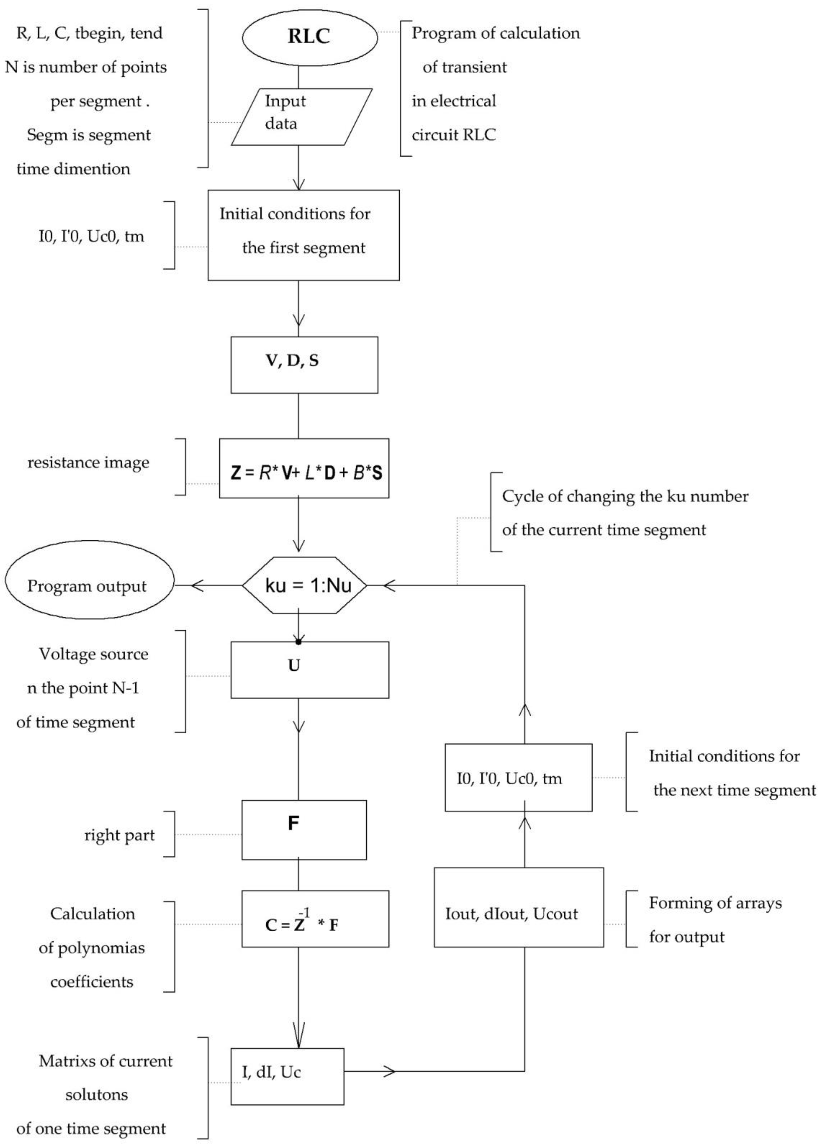
The equivalent circuit for images of current is shown in Figure 2. The block-diagram is shown in Figure 3. The program starts by entering the initial data R, L, C, specifying the interval of simulation tend − tbegin and the dimension of the one-time segment Segm. Then, the initial conditions i₀ and u_C0 are given for the first time segment. The number of segments is defined as the whole part of Nu= (tend − tbegin)/Segm. The program provides a selection of the type of polynomials. For each type, there are features of the formation of matrices V, D, S. There is also a choice of the method of distribution of reference points t: at zeros, at the in maxima of the Chebyshev polynomials, as well as a uniform distribution of points.

The operator resistance $Z=LD+RV+BS$ is calculated. Then cyclic changing of segment number ku from 1 up to Nu is carried out. The calculation error depends on the dimension of the time segment. Choosing a segment dimension for different tasks is done in a trial way. As the segment dimension decreases, the error decreases too.

In each cycle voltage source values are calculated at reference points (vector U), the right-hand side F of Equation (41) is calculated, vector C, the vectors of current values $I=VC+I_0$, current derivative $I^{\prime }=D\cdot C$, the voltage across the capacitor $Uc=B\cdot \left(J\cdot C+I_0\cdot \Delta \right)+U{c}_0$ are calculated. The values of vector elements I, I′, Uc with maximal numbers of nodes of the current segment are determined and they are taken as initial values for the next segment. Calculated values for the current cycle are written to arrays for output. When Nu cycles should be executed, program execution is terminated.

The calculation according to the proposed method was compared with the exact calculation analytically obtained analytically. The program with accompanying subroutines can be freely downloaded from the link [18] and tested in the MATLAB system. The script program is called RLC_ALCH_1_5_10_20_NU.

3. Results

Analysis of the Obtained Calculation Results

The circuit parameters for calculation are given: R = 0.1 Ohm, L = 0.001 H, C = 0.001 F. The voltage source contains the first harmonic with a frequency of 50 Hz and an amplitude E_m1 = 14.1 V, the fifth harmonic E_m5 = E_m1/2, the tenth harmonic E_m10 = E_m1/5 and the twentieth harmonic E_m20 = E_m1/5.

The results of transient calculation using the Chebyshev algebraic polynomials are shown in Figure 4a–c. The reference points were placed in the zeros of the Chebyshev polynomials. The relative deviations of the values of the function of current i_k from the values of i_{anal k} obtained by the exact analytical method, are determined as,$error i=\left(i_{anal k}-i_k\right)/{\left|I\right|}_{\max }$, where |I|_max is the maximum value of the current module.

The time dependence of the function error i is shown in Figure 4d.

Asterisks in the figures show the values obtained by an accurate analytical method. The number of reference points per the segment n = 7. A total of 125 time sections were used. The graph shows that with increasing time value the error does not increase.

To estimate the accuracy of calculations, the relative root-mean-square error deviations are determined. For this purpose, the quadratic deviation of the calculated value of the function of current from the exact value obtained by an accurate analytical method is calculated in the program at each reference point:

$$\Delta i_k={(i_{anal k}-i_k)}^2$$

The mean quadratic deviation is calculated for the entire simulation interval

$$\Delta i_k=\sqrt{\frac{1}{\left(N-1\right)·Nu}{\displaystyle \sum }_{k=1}^{\left(N-1\right)Nu}\Delta i_k}$$

and the relative mean quadratic deviation in percent

$$\Delta i_{otn}\%=\frac{\Delta i}{{\left|I\right|}_{max}}·100\%$$

The errors of the capacitor voltage function and the derivative of the function of current are calculated analogically.

Table 1. Relative mean quadratic deviations of simulating errors in %.

		Algebraic Polynomials			The Tchebyshev Polynomials			The Legendre Polynomials			The Hermite Polynomials
	Simulation Time. s	Zero	Max	Equal Distribution	Zero	Max	Equal Distribution	Zero	Max	Equal Distribution	Zero	Max	Equal Distribution
Δi	0.05	2.75 × 10−4	4.67 × 10−5	3.41 × 10−4	0.73	0.78	1.339	0.95	0.98	1.375	8.44	8.19	7.462
	0.5	2.54 × 10−4	4.66 × 10−5	3.11 × 10−4	0.69	0.73	1.159	0.89	0.91	1.207	6.89	6.71	6.074
Δdi/dt	0.05	1.03 × 10−4	6.06 × 10−6	1.34 × 10−4	0.40	0.46	0.833	0.48	0.53	0.755	5.78	5.60	5.127
	0.5	4.97 × 10−5	5.50 × 10−6	6.16 × 10−5	0.35	0.39	0.621	0.39	0.41	0.526	4.08	3.94	3.567
ΔUc	0.05	3.61 × 10−4	1.79 × 10−5	4.75 × 10−4	1.44	1.65	3.001	1.70	1.89	2.693	20.8	20.3	18.51
	0.5	1.55 × 10−4	1.53 × 10−5	1.95 × 10−4	1.24	1.38	2.230	1.38	1.46	1.857	14.7	14.3	12.91

shows the relative root-mean-square deviations in percent for the function of current Δi, the function of the current derivative—Δdi/dt and the function of the capacitor voltage—ΔUc. The calculations were carried out with a different choice of the method of distribution of reference points: at the zeros of the Chebyshev polynomials, at the maxima of the Chebyshev polynomials, as well as with the uniform distribution of points. Two simulation intervals of 0.05 s and 0.5 s were given. The use of a longer interval 0.5 s makes it possible to evaluate the stabilization process of the calculation. The calculation time on the simulation interval of 0.05 s with the segment duration of 0.0004 s and the number of reference points on into the segment n = 7 is the same in all calculations The processor time of the calculation was estimated with the help of tic, toc operators.

Diagrams of changes in the errors in calculating the voltage across the capacitor when simulating time is equal to 0.5 s are given in Figure 5. As follows from Figure 5, after about 0.1 s, calculation errors decrease and stabilize. The relative mean quadratic error deviations for a simulation time 0.5 s are from 40% up to 99% relative to these errors for a simulation time 0.05 s (Table 1). Error stabilization indirectly indicates the reliability of the obtained analytical expressions and the prospects of using the methods under study for calculating complex circuits.

4. Discussion

The comparison of the errors obtained in calculations by different methods showed the following results. The method using algebraic polynomials is the most accurate. The mean relative quadratic deviations of the current errors were less than 5 × 10⁻⁵%. Errors when using other polynomials were more than 1000 times higher. The lowest accuracy was when using the Hermite polynomials The method of distributing the reference points influenced the accuracy of the calculation. The least errors are in the following distribution methods: algebraic polynomials—in maxima; the Chebyshev and the Legendre polynomials—in zeros; the Hermite polynomials—with a uniform distribution of points.

An increase in the accuracy of calculation can be achieved by reducing the segment size. However, by how many times the segment size decreases, the calculation time increases by the same factor. Increasing the number of reference points n > 7 does not improve the accuracy, but increases the calculation time.

It is possible to provide a simplified explanation of the obtained results. When using other orthogonal polynomials, in comparison with algebraic ones, the coefficients in the expressions representing derivatives and integrals of the currents change significantly. With the equality of the right and left parts of the system of Equation (44), this leads to an increase in errors in the calculation of voltages across each circuit element and the current in the circuit, accordingly.

The calculation time was compared according to the program based on the proposed method and according to the program based on the implicit Euler method of numerical integration of differential equations. The solution of the problem under consideration by the Euler method and its comparison with the solution by the analytical method is given in [19]. This program can be freely downloaded from the specified link and tested in the MATLAB system. The processor time for calculating this program in the MATLAB system (estimated using the built-in function tic, toc) is 6.8 times greater than when using orthogonal polynomials.

The relative mean quadratic current error is 0.85%, that is, it is much larger when orthogonal polynomials are applied. It can be explained as so: Methods for the numerical integration of differential equations calculate sequentially the values at the current step, based on values at the previous steps. In this case, quite a large number of points are used. When using polynomials, the type of solution function is known—polynomial. In the current segment, N − 1 value is calculated at the reference points, and this reduces the calculation time.

The proposed method was also tested to calculate the transient in a more complex circuit. The computer program can be downloaded from the link [20]. The calculation results for this program were verified by comparing the calculations obtained using the multistep Geer method as well as the popular Dommel method.

In conclusion, we note that the development and study of the proposed method for calculating complex nonlinear electrical and magneto-electric circuits of arbitrary complexity will be presented in subsequent publications.

5. Conclusions

• The developed unified spectral method for calculating electromagnetic transients in electrical circuits based on the representation of solution functions by orthogonal polynomials can significantly reduce the simulation time compared with the known methods of numerical integration of differential equations. It is desirable to normalize the segment dimension so that it is close to 1 s. Some researchers consider function approximation of transient by a polynomial to be a risky operation because parasitic oscillations can occur. It is shown that risk is justified if the number of decomposition members is less than 7. The calculation error according to the proposed method can be reduced as you like, reducing the value of the argument segment. Then, the number of segments increases.
• The completed development of the circuit model of the method is convenient for practice.
• The study of the method for algebraic polynomials, as well as the Chebyshev, Hermit and Legendre polynomials, showed that the greatest accuracy is achieved for algebraic polynomials. Errors were more than 1000 times higher when using other polynomials. The method of distributing the reference points influences the accuracy of the calculation.
• Comparison of the calculation time by the proposed method with the implicit Euler method showed that the calculation time decreased by 6.8 times. The calculation of the process in the circuit at a longer time interval showed a decrease and stabilization of errors, which indirectly indicates the reliability of the obtained analytical expressions and the prospects for using the studied methods for calculating complex electrical and magneto-electric circuits.
• The mathematical justification of the proposed method may be interesting for developers of computer modeling programs. For practicing electrical engineers, equivalent circuits and computer programs themselves are of greatest interest.