Development of PMU-Based Transient Stability Detection Methods Using CNN-LSTM Considering Time Series Data Measurement

Abstract

The development of electric power systems has become more complex. Consequently, electric power systems are operating closer to their limits and are more susceptible to instability when a disturbance occurs. Transient stability problems are especially prevalent. In addition, the identification of transient stability is difficult to achieve in real time using the current measurement data. This research focuses on developing a convolutional neural network—long short-term memory (CNN-LSTM) model using historical data events to detect transient stability considering time-series measurement data. The model was developed by considering noise, delay, and loss in measurement data, line outage and variable renewable energy (VRE) integration scenarios. The model requires PMU measurements to provide high sampling rate time-series information. In addition, the effects of different numbers of PMUs were also simulated. The CNN-LSTM method was trained using a synthetic dataset produced using the DigSILENT PowerFactory simulation to represent the PMU measurement data. The IEEE 39 bus test system was used to simulate the model under different loading conditions. On the basis of the research results, the proposed CNN-LSTM model is able to detect stable and unstable conditions of transient stability only from the magnitude and angle of the bus voltage, without considering system parameter information on the network. The accuracy of transient stability detection reached above 99% in all scenarios. The CNN-LSTM method also required less computation time compared to CNN and conventional LSTM with the average computation times of 190.4, 4001.8 and 229.8 s, respectively.

1. Introduction

The development of electric power systems has become more complex due to system interconnection, variable renewable energy (VRE) integration, and distributed generation. It allows the power system utility to operate the system closer to its limits, which means that vulnerable disturbance occurs [1]. If the disturbance is not properly cleared, it can lead to more severe disturbances and the system may suffer blackouts. Several incidents occurred due to failures in the electric power system, such as blackout events in Hokkaido, Japan [2], Canada and the United States [3], South Australia [4], and Europe [5]. One aspect of the stability of the electric power system is transient stability or rotor angle stability [6]. Rotor angle stability is the ability of a synchronous machine in an interconnected electric power system to remain in synchrony after a disturbance occurs.

In addition, most of the power systems in the world still use the supervisory control and data acquisition (SCADA) system, which depends on conventional measurement. The SCADA measures the magnitude of the system variables and collects measurements from the data center. The sampling rate and period among the variables can be different depending on each measurement device’s capability. This condition makes it difficult for the SCADA system to monitor transient events, as presented in [7].

To observe a transient event, a system capable of measuring transient conditions is needed. This feature is fulfilled by the phasor measurement unit (PMU), in which measurement among the PMUs is synchronized. With synchronized measurement, a wide area monitoring system (WAMS) can be built into the power system [1,8,9]. In addition, PMU can also measure phase and magnitude quantities at a high sampling rate; up to 60 per minute. With PMU technology, measurement data can be analyzed to obtain information such as real-time power system network monitoring and control, early warning systems, detection systems, real-time monitoring of voltage, frequency, phase angle stability, and state estimation algorithm improvements [1].

The development of machine learning and deep learning technology has enabled the power system utility to build the application based on historical data. Data collection from protection devices, PMU, smart metering, controllable loads, and communication networks have been mined to develop the technology, as presented in [10]. The application of a machine learning model can be developed into the application of economic load dispatch [11], load forecasting [12], cybersecurity [13], demand response [14], electricity market [15], and stability detection [15]. Even though the computational burden of the machine learning approach is high [7], the machine learning model has advantages because the complete model of an electrical system and its parameters are not compulsory. In addition, there are advantages of synchronized measurement technology regarding the collection of data and information. A machine learning model can be built using a historical event. In each historical event, the PMU measurement can be recorded so that the model would be more precise as a result of the PMU sampling rate capabilities. To detect future events, PMU measurement data can be used as input.

One of the main problems in power systems is transient stability, which can lead to blackouts if not properly cleared. Previous studies have been carried out to detect transient stability. The methods include transient stability analysis with conventional methods, machine learning, and deep learning. Conventional methods such as time domain simulation (TDS), as presented in [16], require complete information on system parameters and fault conditions. Consequently, they are unsuitable for real-time detection of transient stability.

Research in [17] performs transient stability detection by combining binary classification features for transient stability detection and multiclass classification to classify dynamic generator responses. Research in [17] also compared the performance of several methods such as decision tree (DT), ensemble decision tree (EDT), and support vector machine (SVM). The development of other machine learning methods was carried out in research [18]. Research in [18] detects frequency stability using the moving window principal component analysis (PCA) method. In addition, Stockwell’s transform (S-transform) method has also been developed to detect stress stability, as was performed in research [19]. However, the machine learning method has several shortcomings in terms of detecting stability. It is less flexible to different data features. This is because parameter settings depend on the model and data type being created in machine learning modelling.

The next development is using the deep learning method. The deep learning method is a part of the machine learning method that seeks to imitate human neural networks [20]. Deep learning methods are used to extract features in the data and improve the accuracy of the classification process [21]. One of the previous studies has developed a recurrent neural network (RNN)-based method called gated recurrent unit (GRU) [22]. The method was developed to classify transient instability because of short circuit faults. This study has a drawback: not paying attention to the occurrence of loss of synchronism in the generator when experiencing transient instability.

A convolutional neural network (CNN) method was subsequently developed to detect stability. One of the studies developed a continuous online monitoring system (OMS) based on PMU measurements using the CNN method to classify transient instability [23]. Previous research also developed the detection of transient stability by paying attention to two types of transient instability, namely, aperiodic and oscillatory instability [24]. In addition to using CNN for transient stability detection, CNN has also been developed for frequency stability detection [25]. However, the CNN method has disadvantages in detecting transient stability based on time series data because it does not consider the relationship between data series. In addition, CNN requires a long training process because it requires a lot of convolution flow when used to classify data based on time series [26,27].

To overcome the disadvantages of the CNN method, a hybrid method between CNN and RNN was developed as in [28,29]. Research in [28] developed the CNN method in combination with one of the RNN methods, namely, long short-term memory (LSTM) to detect transient stability based on voltage phasor data, whereas research in [29] developed a recurrent graph convolutional neural network (RGCN) method to detect transient stability. However, previous research on the hybrid method between CNN and RNN for the detection of transient stability has not considered the integration of VRE and has not considered delays and topological changes after disturbances occur.

On the basis of previous studies, this research will focus on developing a convolutional neural network—long short-term memory (CNN-LSTM) method to detect transient stability by observing data time-series information, noise, delay, and loss in data and network changes that occur due to disturbances such as line outages, the number of PMUs, VRE integration, and also by paying attention to out-of-step protection on the generator when loss of synchronism occurs. The CNN-LSTM method will be trained using a synthetic dataset generated from the DigSILENT PowerFactory simulation to represent the PMU measurement data. The proposed model will contribute to the detection of transient stability with faster performance, the utilization of time-series data, and the robustness of the power system against noise, delay, and data loss. The proposed model will also consider topology changes due to the contingency event that often occurs after a large disturbance in the power system.

2. Materials and Methods

The method in this study is divided into three stages, namely, data generation, model formation, and detection of transient stability, and ends with a sensitivity test. Data generation is performed to collect synthetic data that will be used to train, validate and test the proposed deep learning model. In the second part, model formation and transient stability detection are carried out. Then in the last part, a sensitivity test of several test parameters such as noise, loss, delay, number of PMUs, and PV penetration rate will be carried out on the proposed CNN-LSTM model.

2.1. Test Case

Transient stability detection simulation needs to be tested on a power system. In this study, the power system used was based on the IEEE 39 Bus system test [30]. In this study, several modifications were carried out, among others, adding a PV system and changing the voltage setpoint values on several buses according to the OPF results. The form of the single line diagram (SLD) used is shown in Figure 1.

The IEEE 39 Bus consists of several components of the electric power system, including 10 generators, 19 loads, 34 lines, 12 transformers, and 39 buses. The number of in the figure denotes the bus. In this study, a 1 PV system was added to bus 2 which replaced the role of the generator on bus 30. The total system capacity was 14.28 GW with a load of 6.13 GW [31].

The PV power capacity used was 600 MW or 10% of the load. However, this study also compared the effect of different PV penetration levels on the transient stability detection results. The PV model used was the standard PV model from DigSILENT PowerFactory. The power control model used was Const. Q, in which the user can specify the active and reactive power output. In this study, the active power was fixed with a power factor value of 1. The dynamic model of the PV system at DigSILENT PowerFactory consists of four main parts, including the photovoltaic block, the DC busbar and capacitor model, the PQ controller, and the static generator model. The PV array is represented by several PV modules that are connected in series and parallel and operate at the maximum power point (MPP). In this study, it is assumed that the ambient temperature and solar irradiation values are constant because the conditions are only observed for a moment meaning the conditions tend not to change. Therefore, intermittent conditions in PV are not considered here. In this condition, the inertia value of the system will affect the transient stability response of the system.

In this research, tests were carried out for scenarios using different numbers of PMUs on the bus, which varied as many as 39, 26, and 13 buses from a total of 39 buses in the power system. Previous research on the number of PMUs has been carried out to ensure that the system is observable [7,32,33]. If the system is observable, the PMU measurement results can represent the system. When the number of PMUs is 39 and 26, systems are still observable. However, when the number of buses is 13 units, there are several buses that are not observable. This research will observe how the number of PMUs used affects the performance of the resulting CNN-LSTM model.

2.2. Data Generation

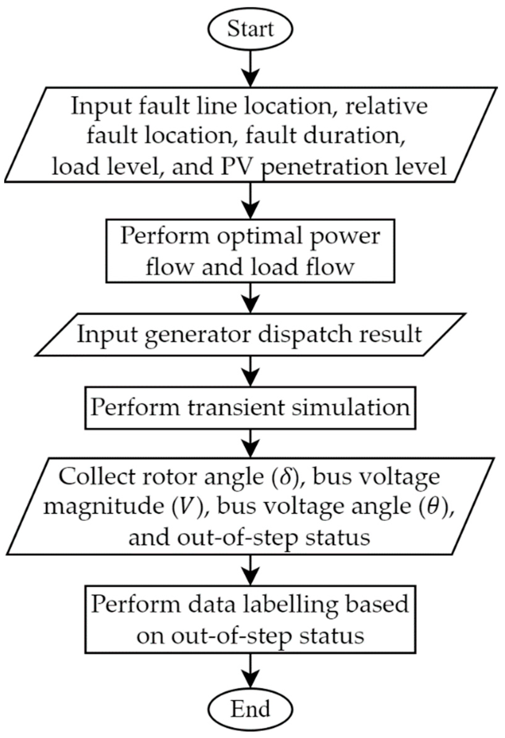
In this section, the PMU data generation and labelling are simulated based on the transient stability conditions. The data generation workflow is shown in Figure 2.

Data generation begins by determining the variation of the operating conditions to be simulated. Variable operating conditions include: the location of the faulted line, the relative location of the faulted line, the duration of the fault, and the load level. Meanwhile, the PV penetration level is fixed. A comparison of the effect of PV penetration level will be carried out in a separate simulation. The variations in operating conditions for each of these parameters are shown in

Table 1. Scenarios of variations in electric power system operating conditions.

Parameter	Description
Location of the faulted line	Each of the 34 lines
Relative location of the faulted line	0%, 20%, 50%, dan 80% from the end of line
Fault duration	0.1 s; 0.15 s; 0.18 s; 0.2 s; and 0.25 s
Load level	70%, 75%, 80%, …, 130% of the IEEE 39-bus standard load demand

.

Furthermore, optimal power flow (OPF) is simulated with the objective function of minimizing network losses and simulating load flow analysis. Both simulations are used to determine the optimal dispatch of each generator with the lowest network losses that meet the operating constraints of the electric power system, as shown in

Table 2. Standard of power system operation [34,35].

Parameter	Value	Unit
Bus voltage	0.9–1.05	p.u.
Transformer loading	100	%
Line loading	100	%
Rotor angle	−180 to +180	deg

, so that the generator output can be set automatically for each variation of load levels via OPF. If the OPF cannot find a solution, then the dispatch condition in the previous variation will be used to ensure that the load flow analysis can run or converge.

After identifying the dispatch generator for each variation of the operating conditions, the next step is to perform a transient simulation. Transient simulation through time-domain simulation is carried out to simulate the transient condition of the operation of the electric power system in a certain time series so that how the system responds when and after a disturbance occurs can be observed. The disturbance simulated in this study is a three-phase short circuit in the line. To produce data labels, tests were used on the value of the rotor angle and critical clearing time (CCT). In this method, it is possible to see whether the value of the rotor angle is outside the range of between −1800 and 1800. If it is outside this range, the system is unstable. In addition, to validate this, the CCT value of the rotor angle response can also be seen. If the disturbance can be removed before the CCT or, in other words, the trouble clearing time is smaller than the CCT, the system is stable and vice versa.

A three-phase short-circuit fault was chosen because this type of fault is the most severe type of short-circuit fault that can occur in transmission lines where the amount of short-circuit current that occurs is the highest compared to other types of short-circuit faults [36]. When there is a disturbance in the line, the disturbance will be eliminated by separating the disturbed line from the network so there is a network topology change in the power system. The system will experience a new equilibrium state in the transient period.

The output of this simulation is the value of the rotor angle (δ), the magnitude of the bus voltage (V), the bus voltage angle (θ), and the out-of-step generator status. The magnitude of the bus voltage and the bus voltage angle were used as input data in deep learning; whereas, the value of the rotor angle and the out-of-step status were used to label the stability condition. When there is an out-of-step on the generator, the system is unstable and vice versa. The data on the magnitude and angle of the bus voltage and the labels generated in this section were inputted in the next section.

2.3. Model Formulation and Stability Detection

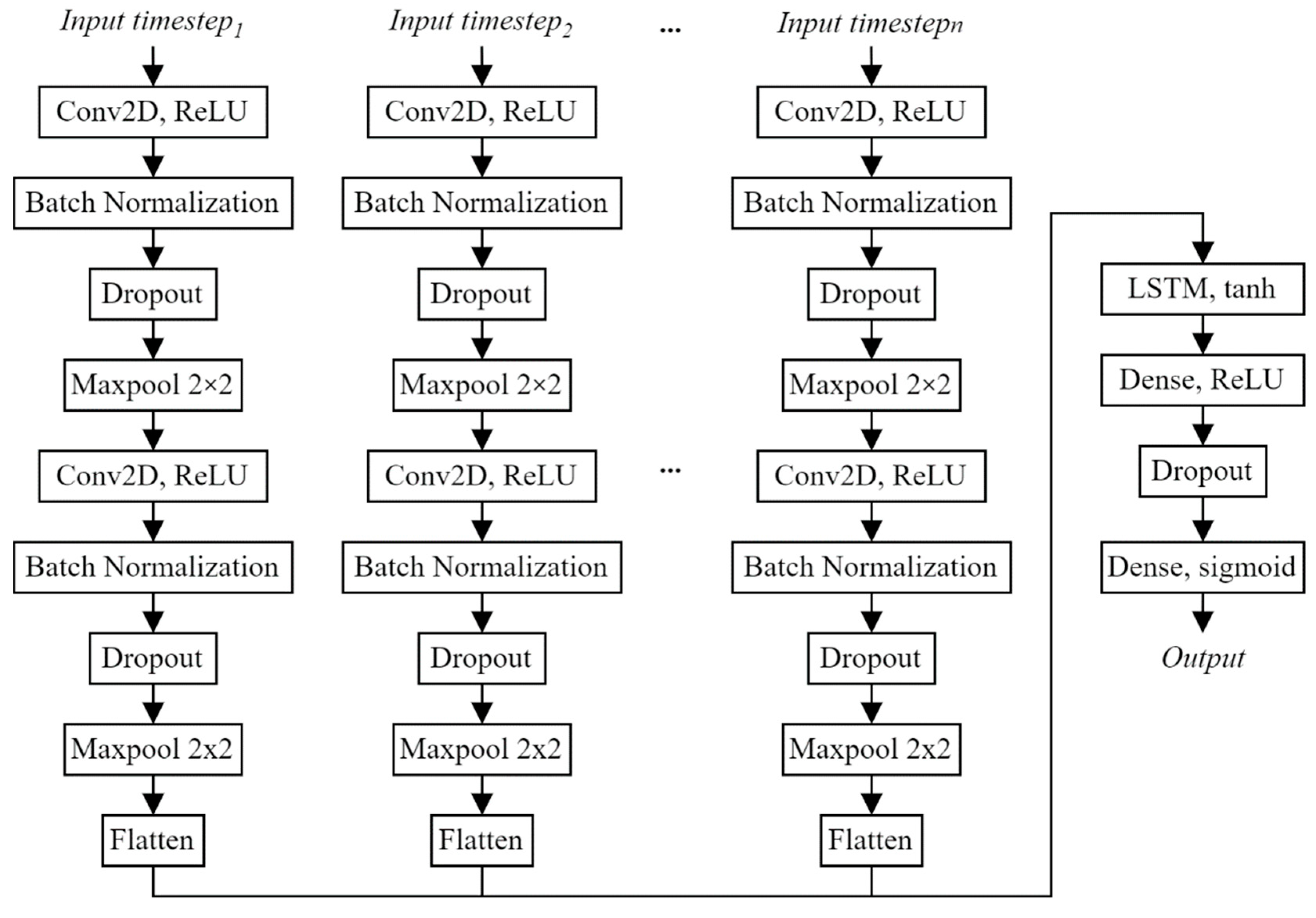
In this study, a hybrid method was used: CNN and LSTM. The CNN layer was used to extract the features contained in the input data, and the LSTM layer was used to support serial data prediction. The CNN method can identify several tensor features based on classes in the network model created. The CNN method has a drawback that it requires a long training time to classify time-series data. This is because it requires several training streams for convolution, namely, one per input image [26,27]. Furthermore, the CNN method cannot detect the relation between time-series connected data streams. By using a time-distributed layer to transform each timestep of data, the same layer is applied to several inputs producing one output per input so that the results are obtained for each time series [37]. Then the output of each time series can be used as input for the LSTM [38]. The architecture used is shown in Figure 3.

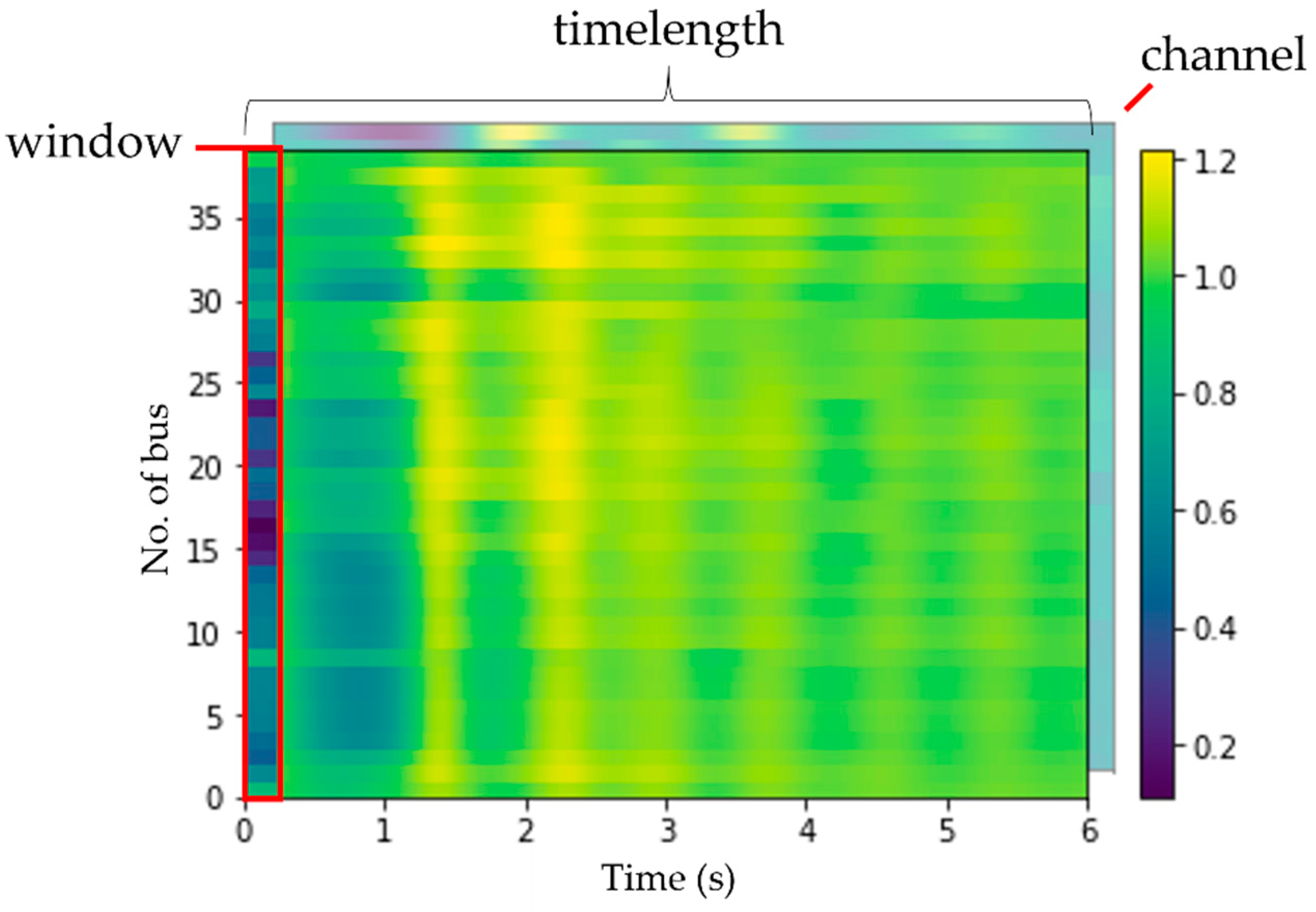
The input form for the method used is illustrated in Figure 4. Several parameters were used, including batch, window, time length, channel, and timestep. Batch shows the set of data samples that are trained at one time. The window shows the data set at each timestep. Time length shows the total data time used in the time-series data. Channel shows the number of channels that contain each type of data. Timestep shows the number of steps performed in each iteration of CNN-LSTM.

The batch size used in this study was 26 units. The window size used was 25 lines of data, and the total time length used was 6 s, which contained 600 lines of data. Then through the window size and time length, the timestep size, which can be seen according to Equation (1), was 24 steps. Furthermore, the size of the channel used was 2 units. Furthermore, for the output form, the method used only consists of batch, size and timestep.

Timestep = time − length/window

(1)

The input data used in this research are voltage magnitude matrix $\left|V\right| \in {ℝ}^{t\times b}$ and voltage angle matrix $\theta \in {ℝ}^{t\times b}$, where $t$ is the number of time samples and $b$ is the number of buses. Then the two matrices are concatenated into a voltage phasor tensor $V \in {ℝ}^{t\times b\times 2}$. A time-distributed layer is used to observe the long-term and short-term time-series features. Therefore, this layer can entirely utilize information in different time frames. Through the time distributed layer, the input data for each time step was analyzed with the same layer architecture as shown in Figure 3.

A filter or convolution kernel convolutes the input tensor to generate feature map output [39]. The convolution operation is represented in Equations (2) and (3) [40]:

$$C\left(i,j\right)=\left(I\ast F\right)\left(i, j\right)$$

(2)

$$C\left(i,j\right)={{\displaystyle \sum }}^{ }{{\displaystyle \sum }}^{ }I\left(i+m, j+n\right)F\left(m, n\right)$$

(3)

where $C$ is the output feature map of size $i\times j$, $I$ is the input matrix of size $i\times j$, and $F$ is the convolution kernel of size $m\times n$.

The feature map output is then executed with the ReLU activation function, which maps the input to 0 or maintains the value constant. If the value is negative then it is mapped to 0; whereas, if it is positive the value will remain. The ReLU activation equation is shown in Equation (4). The activation function is required to generate non-linearity [39] so that deep learning classification can be done.

$$f\left(x\right)=\max \left(0,x\right)$$

(4)

where $f\left(x\right)$ is the activation function and $x$ is the matrix element input.

A batch normalization layer is used to perform normalization of the input. Batch normalization can transform input so that the mean output ${\mu }_B$ remains near zero and the standard deviation ${\sigma }_B$ remains near to 1. Batch normalization formulations are shown in Equations (5)–(7) as follows:

$${\mu }_B=\frac{1}{m}{\displaystyle \sum }_{k=1}^m{x}_k$$

(5)

$${\sigma }_B=\sqrt{\frac{1}{m}{\displaystyle \sum }_{k=1}^m{\left(x_k-{\mu }_B\right)}^2}$$

(6)

$$x_k^{\prime }=\frac{x_k-{\mu }_B}{{\sigma }_B}$$

(7)

where ${\mu }_B$ and ${\sigma }_B$ are the mean output and standard deviation in every batch, respectively. Then, $m$ is the number of the sample, and $x_k^{\prime }$ is the normalized input. Batch normalization processes are different between training and testing. In the training process, the layer normalizes the output using the mean and standard deviation from the inputted batch. On the other hand, in the testing process, the layer uses a moving average from the average and standard deviation to normalize the output from the batch from the testing stage.

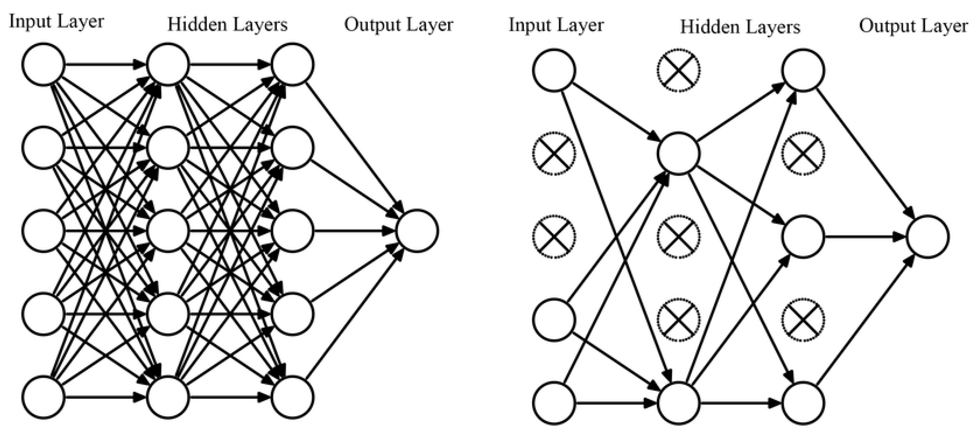
A dropout layer would randomly adjust the input unit to 0 using a specific value of frequency in each training process. Another nonzero input would be scaled to 1/(1 − rate) so that the number of the input remained the same. Illustrations of the dropout layer process are presented in Figure 5. The arrow denotes the process direction from the input, model. and the predicted output. The dropout layer is useful to prevent overfitting in the model [39].

A maxpool layer was used to perform a down sampling operation, which reduces the element number from the feature map. The element is then used as input for the pooling layer. In this research, the down sampling of the feature map was performed based on the maximum in the pool.

A flatten layer was used to change the tensor input in the form of $\left(n, c, h, w\right)$ into a vector with the dimension $\left(n\times c\times h\times w\right)$, where $n$, $c$, $h$, dan $w$ are the number of batches, channel, column, and row. This layer was used to produce the input that was able to be processed by the LSTM in the next step.

The LTSM layer contains a memory block consisting of cell state and gate state for the recurrent process. In this research, the activation function is tanh, and the recurrent process is sigmoid. The formulation of tanh and sigmoid activation function is presented in Equations (8) and (9).

$$f\left(x\right)=\frac{e^x-e^{-x}}{e^x+e^{-x}}$$

(8)

$$f\left(x\right)=\frac{1}{1+e^{-x}}$$

(9)

Dense layers/fully connected layers will operate the input based on the activation function used. In this research, there are two dense layers. The first one is the ReLU function after the LTSM, and the second one mapped the probability prediction form neural network using the sigmoid. The sigmoid was chosen because the predicted target class is binary. Finally, the deep learning output in the vector form shows the prediction output in each timestep. The prediction has two classes: stable and unstable.

The loss function is a function that is used to measure how well the prediction or output produced performs against the expected target. In this research, the binary cross entropy loss function was used. This function was used because in this research the predictions made are binary (0 and 1). Binary cross entropy is preceded by a sigmoid activation function. The equation for binary cross entropy is shown in Equation (10):

$$loss=-t_{i}log\left(y_i\right)-\left(1-t_i\right)log\left(1-y_i\right)$$

(10)

where $t_i$ is the target class on the $i$-th element and $y_i$ is the prediction output generated by the neural network algorithm on the $i$-th element.

3. Simulation Results

The simulation results were analyzed and discussed by observing the data generation process and by comparing results among the methods, parameter control and data quality. Data generation was performed by observing the number of each class and each class representation using a colormap. Then in the method comparison, parameter control and data quality aspect, the simulation results of each scenario variation were observed depending on the method used and the deep learning parameter.

3.1. Data Generation and PV Penetration Effect

In this section, the data generation for each class is compared to identify the data number and representation. Furthermore, the network topology with different penetration PV levels of three scenarios are also compared. The amount of simulated data for each scenario are shown in

Table 3. Generation data of PV penetration effect representation.

Scenario	Number of Data		Training	Validation	Testing
	Stable	Unstable	Accuracy (%)	Accuracy (%)	Accuracy (%)	F1-Score
Without PV	29,356	2468	99.75	99.80	99.76	0.9987
With PV 10%	29,605	2219	99.85	99.94	99.89	0.9994
With PV 15%	28,726	3098	99.95	99.99	99.93	0.9996

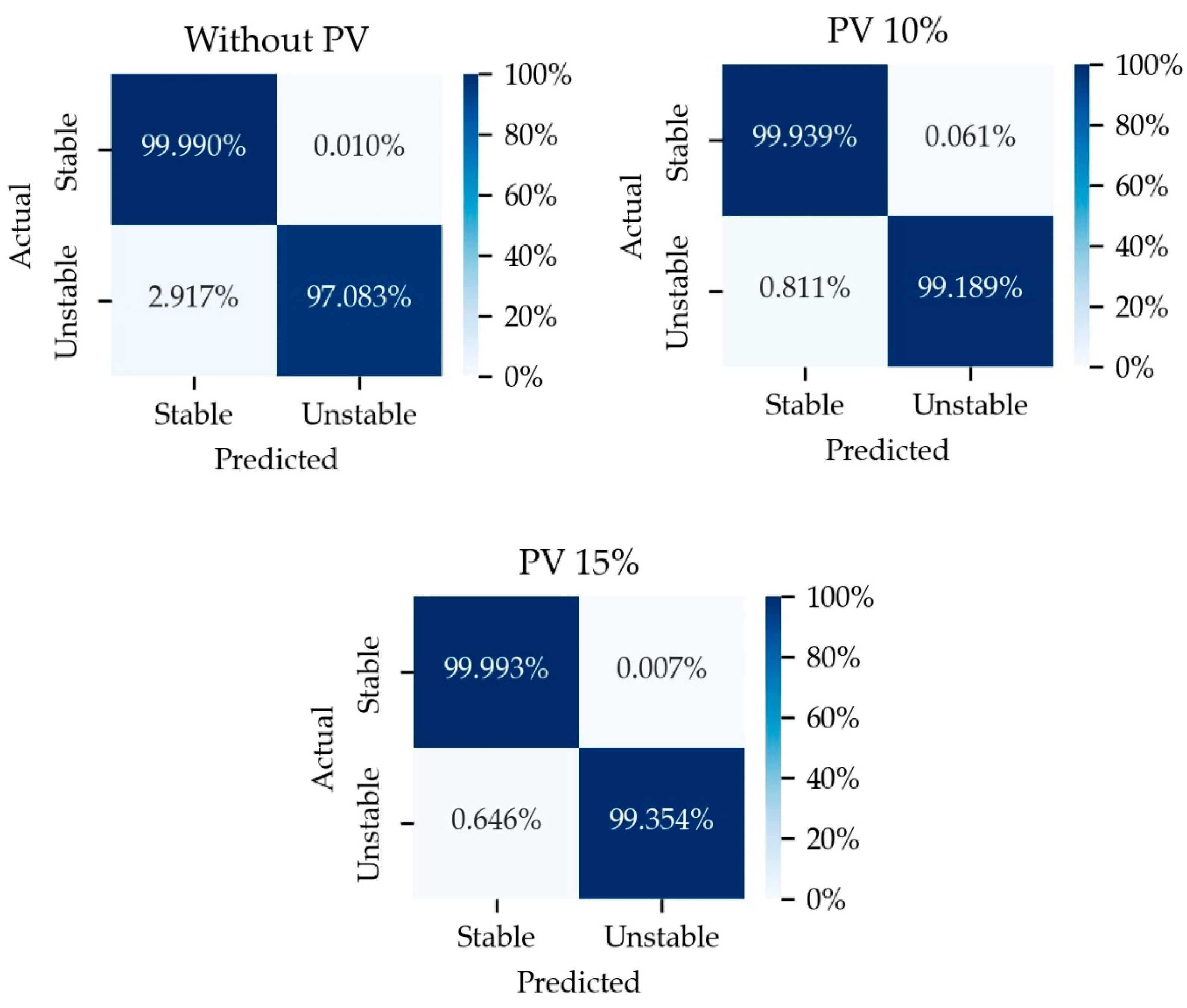
. Data classification from Table 3 was obtained from the data labelling process. Data labelling detects whether generating units go out of step or not. The rotor angle has a transient stability operation limit between −180° and 180°. When the rotor angle reaches –180° or 180°, the internal synchronous generator rotor angle would go in to the out-of-step phase from the reference voltage point of view. Generator voltage and current would oscillate following the rotor angle oscillation between −180° and 180°. When the rotor angle is unstable, the operating condition is called critical clearing time (CCT). In the simulated power system, clearing time of the disturbances/faults would gradually increase to find a generator in the out-of-step condition (CCT). CCT would be compared to the clearing time in the data generation process simulation. When the fault can be cleared before the CCT or the fault clearing time is less than the CCT, the system is stable, otherwise, the system is unstable. The resulting normalized confusion matrix is shown in Figure 6.

As shown in Table 3, the PV penetration level in the system can affect the transient stability of a power system [42,43]. Depending on the network topology and the system operation, PV penetration can strengthen or weaken the system’s transient stability. When the PV penetration is 10% of the peak load, the number of stable operating conditions rises. However, when the penetration is 15%, the number of stable operation conditions decreases. This is also proven in [43]. The research in [43] analyzed the transient impact of the VRES according to the future Korean power grid scenario. The results of the research show that transient stability increases when the RES penetration is small. However, when the penetration level increases, the transient stability decreases. This is related to the increasing imbalance of supply and demand load by RES penetration. The area associated with an increase in power generation due to RES penetration is not the same as the area associated with a decrease in power generation due to RES penetration. Another researcher in [44] also analyzed transient stability as a result of the integration of a solar farm on the grid. The research in [44] conducted a transient stability test using the IEEE 9 bus system by taking into account the effect on the CCT value. This study shows that PV penetration leads to a decrease in the CCT value. When a conventional generator is turned off, the CCT value increases slightly. The smaller the CCT value, the more vulnerable the system is to instability. Thus, the presence of PV penetration can make the system more unstable or more stable depending on the operating conditions of the conventional generator in the system, which will affect the balance of power and load on the system and the flow of power distribution from the generator to the load.

In this research, the operating condition for each case was randomly generated based on possible actual operation conditions. It occurs because the PV penetration in the 15% case violates the power system regulations due to the voltage profile and power system component loading. Moreover, based on the accuracy and F1-score, the best ranking conditions for detecting transient stability are with PV 15%, with PV 10% and without PV.

3.2. Model Formulation and Transient Stability Detection

In this section, the hyperparameter values in the CNN-LSTM model are compared, analyzed and discussed. The hyperparameter values are presented in

Table 4. Hyperparameter testing scenario [30,45,46,47,48].

Scenario	Hyperparameter Value
	Conv2D_1	Conv2D_2	Conv2D_1	Dense	Conv2D_1
1	4	8	16	16	0.2
2	4	8	16	16	0.5
3	4	8	16	16	0.8
4	8	16	32	32	0.2
5	8	16	32	32	0.5
6	8	16	32	32	0.8

. The training, validation and testing results are presented in

Table 5. Recapitulation of hyperparameter testing results.

Scenario	Training	Validation	Testing
	Accuracy (%)	Accuracy (%)	Accuracy (%)	F1-Score
1	99.70	99.81	99.79	0.999
2	99.56	99.74	99.67	0.998
3	97.37	99.53	99.35	0.996
4	99.85	99.94	99.89	0.999
5	99.70	99.63	99.55	0.998
6	99.40	98.84	98.58	0.992

.

Based on the accuracy and F1-score, the optimal model is the model in scenario 4. For this reason, the hyperparameter in scenario 4 was used in the following model in this research.

3.3. Sensitivity Test

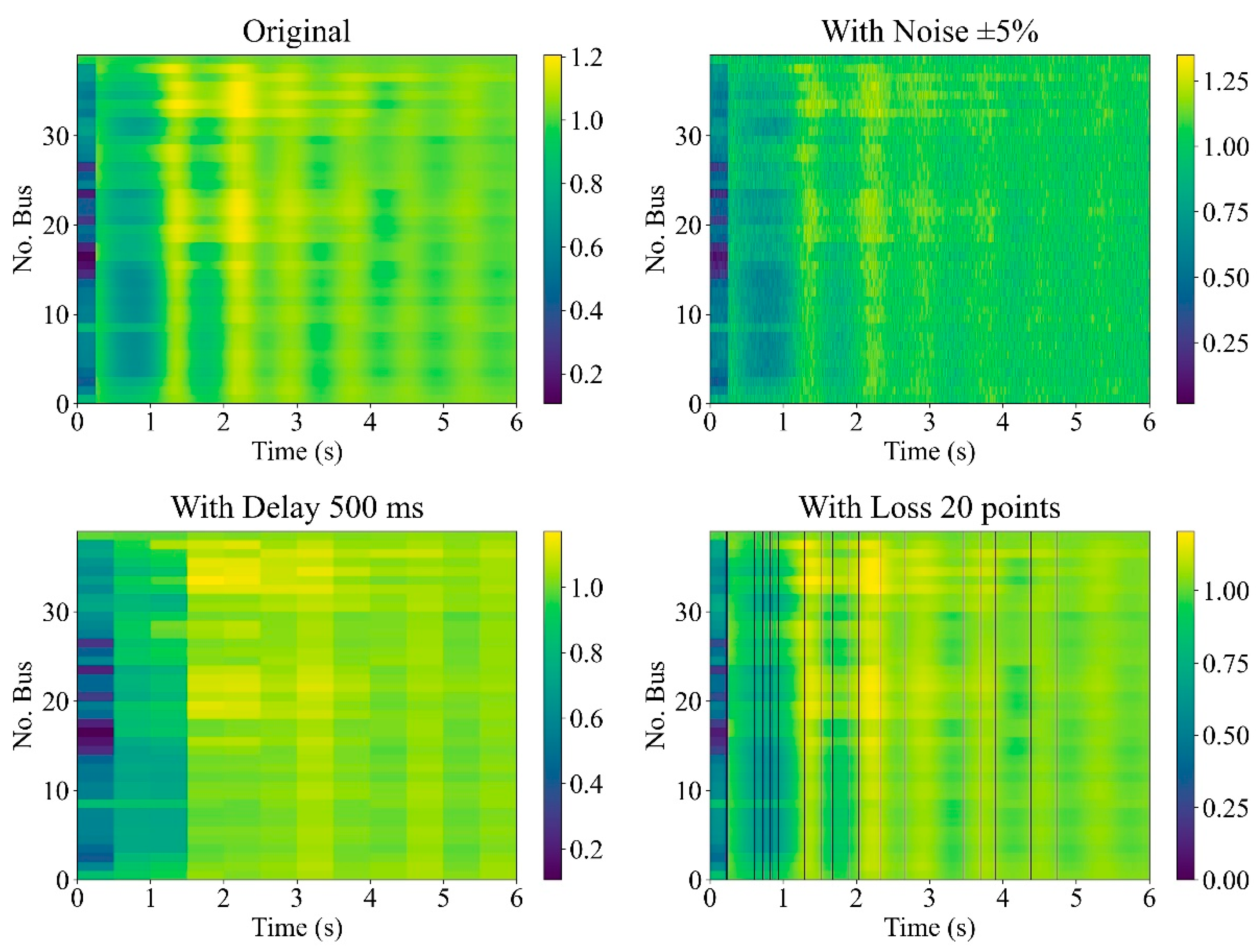
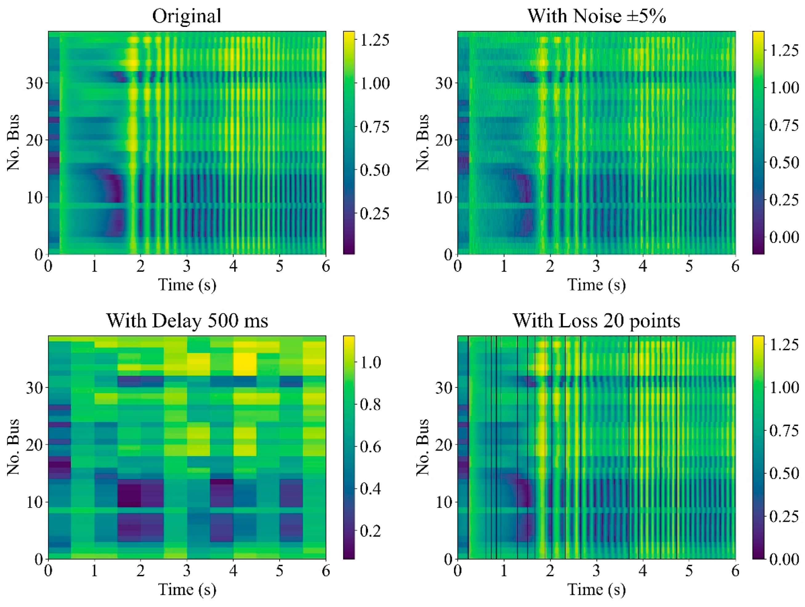
The quality of the data used to train a deep learning model can affect the resulting performance. In this section the effect of PV penetration level, data quality such as noise, loss, delay, and the number of PMUs used are analyzed. Noise, delay, or loss in the measurement data is generated before conducting the CNN-LSTM training process. Therefore, the characteristics of CNN-LSTM detection results when there is data that has noise, delay, or measurement loss can be observed. Illustrations of the data in the form of a voltage magnitude response using a colormap for data with noise, delay, or loss when conditions are stable and when conditions are unstable are shown in Figure 7 and Figure 8, respectively.

In addition, comparisons with similar methods were also analyzed. To avoid the influence of other parameters in testing the sensitivity of certain parameters, the other parameter values were maintained at the same level. Simulation results were obtained from 13 PMU, 10% PV penetration, 1% PMU measurement noise, data losses in 10 buses, and a delay of 100 ms. The estimated optimal number of PMUs was set as 30% of the number of buses. Moreover, the performance of the detection results using testing data can be seen. The analysis was performed by looking at the confusion matrix generated by data testing. The performance parameters used include accuracy and F1-score.

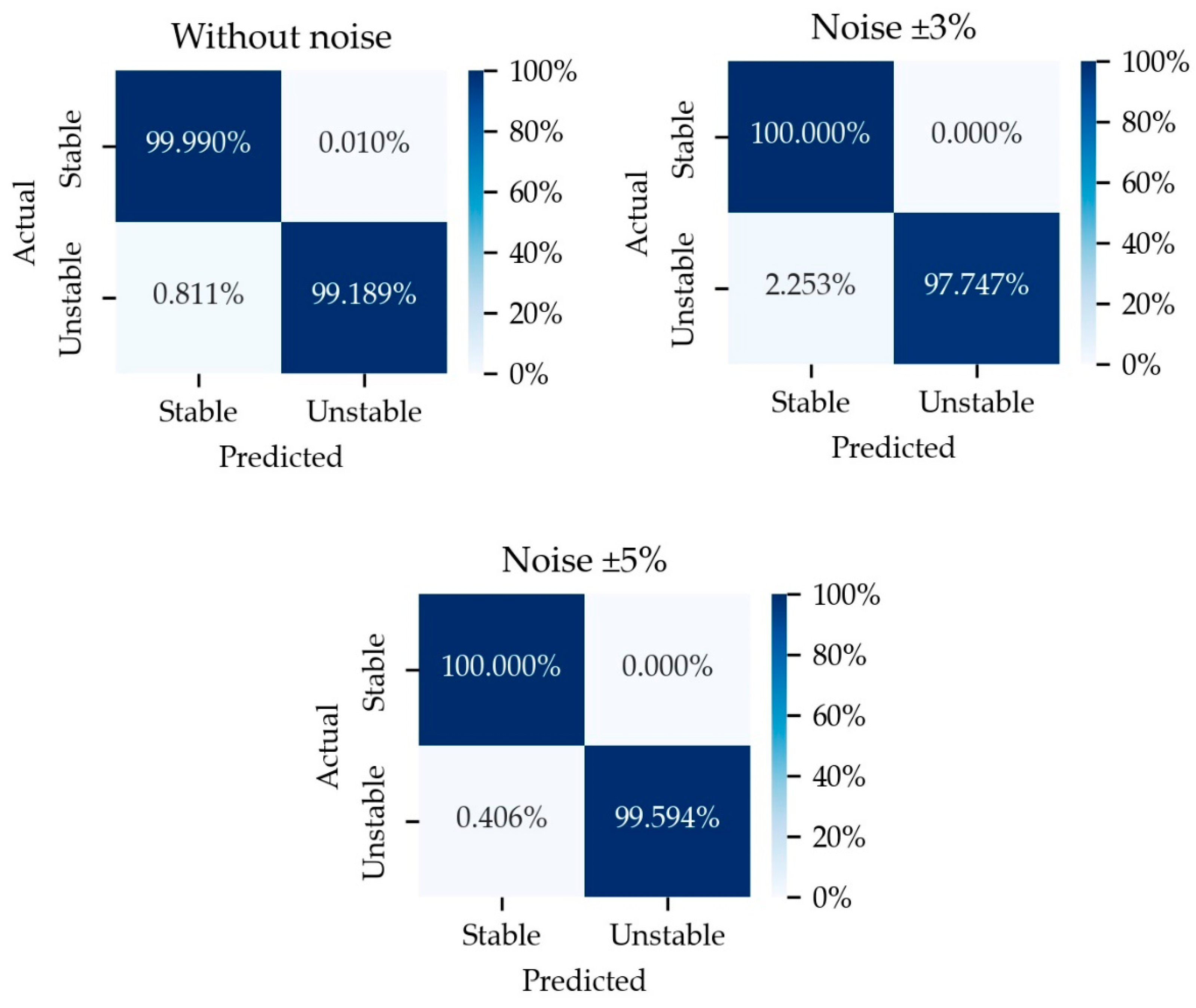
3.3.1. Effect of Noise

In order to observe the noise effect on the prediction, three noises levels were generated. The results of training, validation, and testing of some noise levels are shown in

Table 6. Recapitulation of test results for the effect of noisy data.

Noise Level	Training	Validation	Testing
	Accuracy (%)	Accuracy (%)	Accuracy (%)	F1-Score
±0%	99.96	99.91	99.93	0.9996
±3%	99.91	99.94	99.84	0.9992
±5%	99.90	99.90	99.97	0.9998

. The resulting normalized confusion matrix is shown in Figure 9.

The noise is generated by randomly generating noise of a voltage magnitude and angle different from the actual value. This makes the model process different data according to the noise level. The presence of noise in the data used can affect the performance of the resulting model. The accuracy of the training process decreased when the noise level increased. However, in the validation and testing process, the resulting model did not have a certain trend towards noise.

3.3.2. Effect of Data Loss

In order to observe the effect of data loss on the prediction, three levels of data missing were generated. The results of training, validation, and testing are shown in

Table 7. Recapitulation of test results for the effect of data loss.

Number of Missing Data Points	Training	Validation	Testing
	Accuracy (%)	Accuracy (%)	Accuracy (%)	F1-Score
0	99.96	99.91	99.93	0.9996
10	99.94	99.89	99.89	0.9994
20	99.93	99.98	99.96	0.9998

. The resulting normalized confusion matrix is shown in Figure 10. The number of data rows used in this study was 600 data rows with a window size of 25 rows of data and a batch size of 26 units.

With the missing data, the magnitude and angle of the voltage in the data used will change the data pattern. This makes the model process different data according to the number of missing data points so that the performance of the resulting model does not have a certain trend toward the number of missing data. Similarly to the data noises, the accuracy is decreased only in the training process. Generally, the number of missing data points at this level does not affect the accuracy.

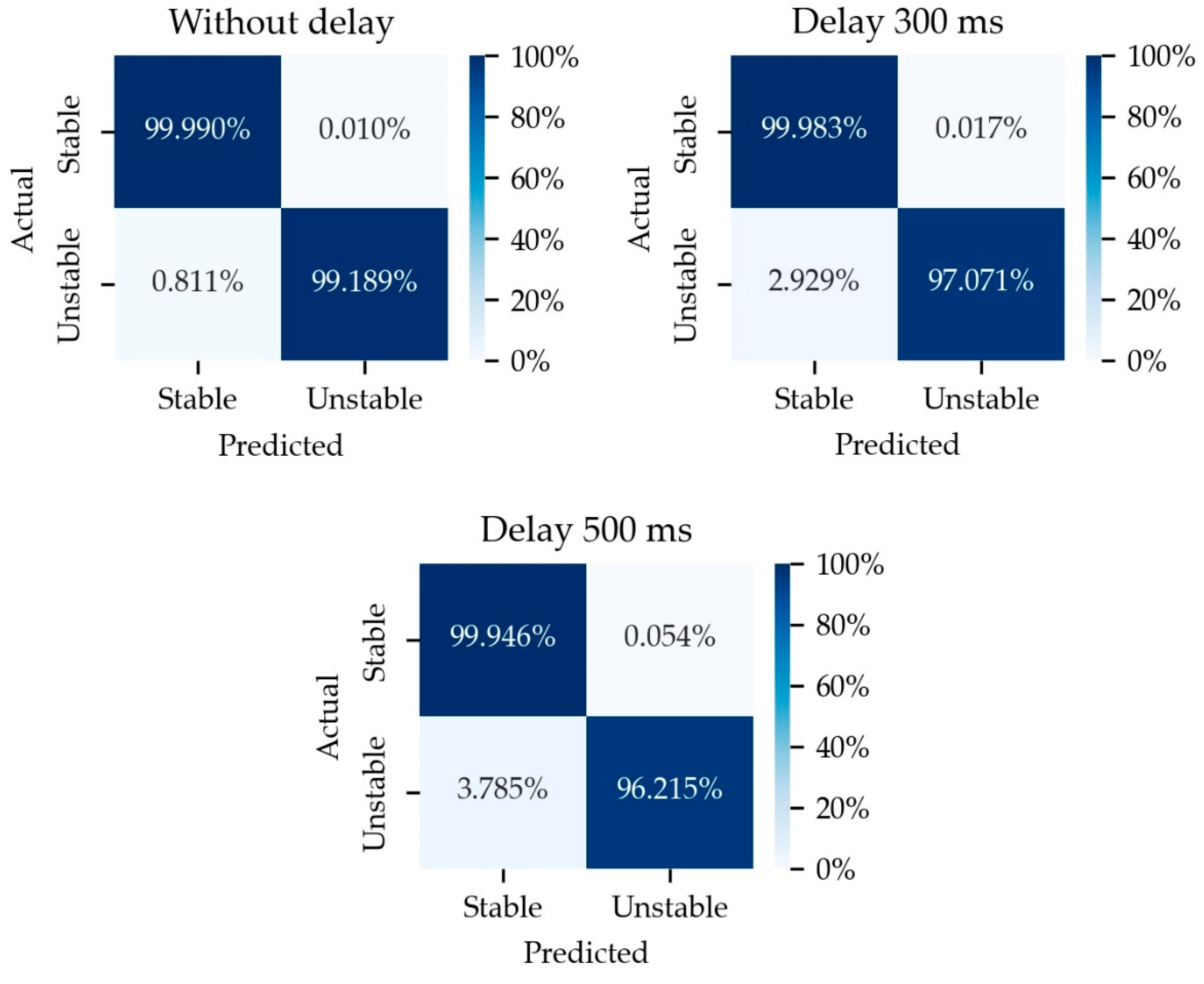
3.3.3. Effect of Delay on Data

In order to observe the effect of delayed data on the prediction, three levels of delay were generated. The results of training, validation, and testing are shown in

Table 8. Recapitulation of test results for the effect of delayed data.

Delay	Training	Validation	Testing
	Accuracy (%)	Accuracy (%)	Accuracy (%)	F1-Score
0 ms	99.96	99.91	99.93	0.9996
300 ms	99.84	99.82	99.78	0.9988
500 ms	99.68	99.67	99.69	0.9983

. The resulting normalized confusion matrix is shown in Figure 11.

The greater the delay, the worse the performance of the resulting deep learning model will be. This can happen because the amount of delay makes the value of the data in the delay time range the same, which makes the data pattern more difficult to identify. Thus, the delay in the data used can affect the performance of the resulting model.

3.3.4. Effect of The Number of PMU

In order to observe the influence of the number of PMU on the prediction, three levels of the number of PMU were generated. The results of training, validation, and testing are shown in

Table 9. Recapitulation of test results for the effect of the number of PMUs.

Number of PMUs	Training	Validation	Testing
	Accuracy (%)	Accuracy (%)	Accuracy (%)	F1-Score
13	99.92	99.95	99.96	0.99978
26	99.92	99.97	99.96	0.99980
39	99.98	99.99	99.99	0.99997

. While the resulting normalized confusion matrix is shown in Figure 12. The resulting normalized confusion matrix is shown in Figure 12.

Overall, although the number of PMUs is limited to 30% of the total buses on the system, in the case of 13 buses out of 39 buses, the model still has an accuracy of above 99%. Furthermore, the number of PMUs used in the data can affect the performance of the resulting model. The greater the number of PMUs used, the better the performance of the resulting model.

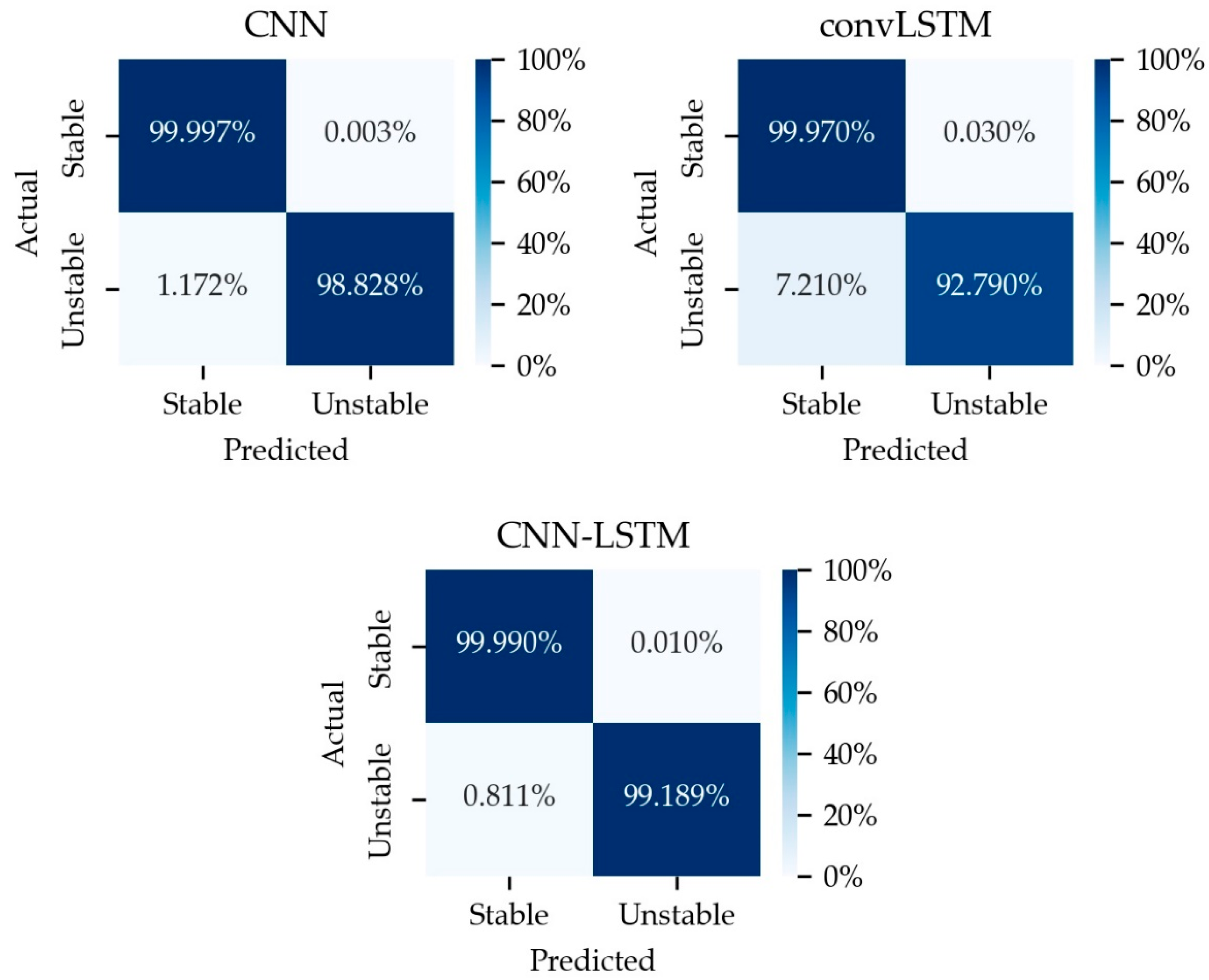
3.3.5. Comparison of CNN, convLSTM, and CNN-LSTM Methods

This section analyses and discusses the comparison of several methods, including CNN, convLSTM, and CNN-LSTM. The results of training, validation, and testing are shown in

Table 10. Recapitulation of test results for comparing deep learning methods.

Methods	Training	Validation	Testing
	Accuracy (%)	Accuracy (%)	Accuracy (%)	F1-Score
CNN	99.90	99.93	99.92	0.9995
convLSTM	99.47	99.54	99.47	0.9972
CNN-LSTM	99.96	99.91	99.93	0.9996

. The computational time required is shown in

Table 11. Computational time for comparing deep learning methods.

Method	Number of Epoch	Simulation Time (Second)
		Total	Minimum	Maximum	Average
CNN	20	80,035	3953	4531	4001.8
convLSTM	20	4595	228	236	229.8
CNN-LSTM	20	3807	189	193	190.4

. The resulting normalized confusion matrix is shown in Figure 13.

On the basis of the simulation results, the CNN-LSTM method can solve the problem of the large time consumption of the CNN method and reduce the computational time of the convLSTM method when implemented to predict multiple time-series data. Thus, the CNN-LSTM method has the best performance and the fastest computation time compared to the CNN and convLSTM methods.

4. Discussion

The proposed method has the capability to detect transient stability conditions from only the voltage angle and magnitude of the respected bus, without considering the network parameters with high accuracy. The accuracy of the training process is 99.85%, validation is 99.94% and testing is 99.89%. The F1-score from the data testing is 0.999.

VRE penetration effect also affects the accuracy. In this research, the PV was simulated in the test system. The penetration level of PV caused changes in the number of stable and unstable conditions under similar simulated conditions. In this research, the tradeoff between accuracy and the VRE penetration level was not observed. However, the proposed method can produce 99% accuracy.

Data quality also affects the accuracy of the detection. In the daily power system operation, noise and data losses often occur, which change the data pattern. Moreover, there is also a communication delay that occurs in the operation which means that the pattern cannot be easily recognized. The proposed method can still produce 99% accuracy until a certain level of noise, delay, and data loss, as shown in

Table 12. Summary of sensitivity test.

Sensitivity Test	Testing
	Accuracy (%)	F1-Score
Noise ± 5%	99.97	0.9998
Data Loss: 20 points of 600 points	99.96	0.9998
Delay 500 ms	99.69	0.9983
Number of PMU: 13 buses of 39 buses	99.96	0.99978
PV Penetration 15%	99.93	0.9996

. In this research, 5% noise, 20 nodes of data losses and 500 ms delay were still acceptable.

The proposed method has not only high accuracy, but also faster computational time compared to CNN and conventional LSTM. The proposed method can speed up the computational time of CNN and improve the accuracy of LSTM, as shown in Table 11.

5. Conclusions

The proposed method was developed using CNN-LSTM that requires a tradeoff between high prediction accuracy and faster computation time. The main procedure of the proposed method is data generation of the simulated power system, model formulation, a training process to formulate the model, a testing process to validate the model and the classification of the results.

In systems with high penetration of VRE, the transient stability problem would be different from the traditional one. High penetration of VRE would increase instability. If all possible labelling data are available, even in the power system operation, transient stability detection can still provide high accuracy. Consequently, the training process for higher VRE penetration should be performed when the VRE generating unit is installed.

The effect of the data input quality on the accuracy of the proposed method should be elaborated more. The number of PMUs in the power system would affect the quality of the data input in the proposed method. The optimization of the PMU number in a power system would be an interesting subject to pursue to improve accuracy. Optimization can also include the network topology change because the system should fulfil the N-1 contingency criteria. If the power system needs to be expanded by adding a new generating unit and transmission line, the model should be adjusted.

Currently, this method works well under the specific test system with the accuracy above 99% for all scenarios. The CNN-LSTM method also required less computation time compared to CNN and the conventional LSTM with the average computation time 190.4, 4001.8 and 229.8 s, respectively. If this method is applied to real power systems, the implementation of each step would be challenging to apply. The process should start with identifying the system, the characteristics of the generating unit, the transmission line characteristics, the load characteristics, the disturbances record and the intermittent characteristics of VRE. After that, each step of the proposed method can be built including data pre-processing, setting of the hyperparameter values, data labelling, training and testing.