Perspective

Perspective of Thermal Analysis and Management for Permanent Magnet Machines, with Particular Reference to Hotspot Temperatures

Department of Electronic and Electrical Engineering, The University of Sheffield, Sheffield S1 3JD, UK
*
Author to whom correspondence should be addressed.
Energies 2022, 15(21), 8189; https://doi.org/10.3390/en15218189
Submission received: 6 October 2022 / Revised: 23 October 2022 / Accepted: 28 October 2022 / Published: 2 November 2022

Abstract

:
Permanent magnet (PM) machines have been extensively used for various applications. Nevertheless, thermal effect, particularly hotspot temperature, not only severely restricts power/torque density but also leads to deteriorations in electromagnetic performance, service life, and reliability. Starting with foundations of PM machines and heat transfer mechanisms, this paper reviews the development of thermal analysis methods over the last thirty years and the state-of-the-art research achievements, and the hotspot temperatures of winding and PM are particularly evaluated. In the overview, various machine losses and cooling techniques are first introduced, which are the essential reasons for temperature rise and the most straightforward way to remove the generated heat. Afterwards, the mainstream thermal analysis techniques, i.e., numerical techniques, lumped-parameter thermal model, and hybrid thermal models, as well as the online electrical parameter-based and thermal model-based temperature monitoring techniques, are reviewed and assessed in depth. In addition, this paper also reviews the analytical thermal modelling methods for winding and PM. Finally, future research trends are highlighted.

1. Introduction

Electrical machines account over 40% of global electricity consumption [1] and play a critical role in both industries and economics. As the evolution of rare-earth permanent magnet (PM) materials [2], the maximum energy products of neodymium iron boron (NdFeB) magnets can achieve towards 500 kJ/m3, Figure 1. Therefore, PM machines can offer high overall efficiency and torque density, and thus, have been extensively used in numerous applications, e.g., aerospace [3], household appliance [4,5], electric/hybrid electric vehicle [6], and wind power generation [7], etc.
Generally, the thermal effect is one of the key factors restricting the increase of power/torque density, especially for the induction and PM machines [8]. On the one hand, the winding insulation will be deteriorated when the local hotspot temperature exceeds the maximum allowed operating temperature. The maximum operating temperature depends on the winding insulation class and is typically <180 °C [9]. Consequently, the degradation of wire insulation could further cause short circuit faults and eventually cause machine failure [10,11]. On the other hand, the thermal deterioration is even more crucial for PM machines since the widely used high energy rare-earth PM material, i.e., NdFeB, is sensitive to overheating. With the increase of PM temperature, the decreasing remanent flux density and the reduction of knee points of PM demagnetization characteristics will reduce output torque capacity and efficiency. More severely, when the local PM hotspot temperature exceeds the maximum allowed operating temperature and the working points operate beyond the knee points of PM demagnetization characteristics, it will cause partial irreversible PM demagnetization. Furthermore, when the PM temperature reaches the Curie temperature, PMs will be fully demagnetized. Table 1 lists the physical properties of some common PM materials, where B and H c J are the remanent flux density and the intrinsic coercive force, respectively. B H max is the remanent flux density. ϑ max is the maximum operating temperature. α B r and α H C are the temperature coefficients of the remanent flux density and the coercive field strength, respectively. ρ is the electrical resistivity.
Although thermal analysis is important for PM machines, it has obtained less attention compared to electromagnetic analysis in the last few decades. This may be attributable to the fact that machine designers may lack a thermodynamic background [13]. More recently, especially in the new century, the importance of the thermal effect has been more well known, and much more effort has been put into the development of thermal analysis [13,14,15,16,17,18,19,20,21,22,23,24,25,26,27,28,29,30,31,32,33].
Reviewing the evolution of thermal analysis for electrical machines in last few decades, thermal analysis methods, including lumped-parameter thermal models (LPTMs) [34,35,36,37,38,39] and finite element methods (FEMs) [40,41,42,43,44,45], have been employed as early as the 1990s, but were primarily concerned with the induction machines (IM). Meanwhile, the implementation of FEM at that time was complicated and mainly relied on manual programming due to computer hardware limits.
In the first decade of the 21st century, with the popularity of PM machines, the thermal analysis for PM machines garnered much more attention [13,14,15,16,17,18,46,47,48,49,50,51]. The numerical techniques, including electromagnetic-thermal coupled FEM (ETFEM) and computational fluid dynamics (CFD), were maturely programmed in the software and then become one of the most powerful analysis tools [18,47,48,49,50,51,52,53]. LPTMs that were initially modelled for IMs have also been widely applied to PM machines [38,46,47,48,49]. In addition, the LPTM based commercial thermal analysis software Motor-CAD [54] was also developed in 1999 and then further widely employed [13,14,15,16,17,18,19].
From the 2010s, the hybrid thermal models incorporating LPTM with CFD [55,56,57], FEM [58], or the analytical thermal model (ATM) [53,59,60,61,62,63,64,65,66] have been developed to synergize the respective advantages. Meanwhile, several online temperature estimations, including electrical parameter-based [67,68,69,70,71,72,73,74,75,76,77] and thermal model-based techniques [78,79,80,81,82,83,84,85], have also been developed. In addition, machine learning-based neural networks have also been used for thermal monitoring [86,87] recently. In summary, the development of thermal analysis for electrical machines since the 1990s is briefly outlined in Figure 2. In addition, a detailed list of references with remarks is listed in Appendix A.
To date, to help researchers and machine designers be familiar with the thermal analysis of electrical machines, several excellent review papers, e.g., [13,14,15,16,17,18], have been published in the 2000s. However, as aforementioned, numerous new techniques in thermal analysis techniques have been developed over the last 10 years or so which are also worth reviewing and evaluating. More recently, many survey papers have reviewed various cooling techniques specific to different applications, such as wind power generation [19], aerospace [20,21], automotive [22,23,24], advanced manufacturing techniques [28,29], etc., which are summarized in Table 2. Obviously, common cooling techniques have been extensively reviewed so far, while the accurate estimation of machine temperatures, particularly hotspot temperatures of winding and PM, are equally or even more important. Nevertheless, the recently developed thermal analysis and temperature estimation techniques, e.g., analytical thermal modelling, the hybrid thermal model, and grey/white thermal model-based online temperature estimation still remain to be reviewed and assessed. Meanwhile, instead of average temperature prediction, hotspot temperature estimation becomes one of the current areas of research, but has not been reviewed so far.
Therefore, with particular reference to hotspot temperatures within electrical machines, this paper reviews the development of thermal analysis and management techniques in the last few decades together with their basic working principles. Meanwhile, mainstream cooling methods, thermal analysis and online temperature estimation methods are also assessed from various perspectives, with specific attention to their effectiveness of hotspot temperature reduction or capabilities of hotspot temperature prediction. The aim is to help readers establish an overall understanding of the state-of-the-art development and challenges, as well as their perspectives in this field.
This paper is organized as follows. Section 2 introduces the foundations of PM machines and heat transfer mechanisms. Section 3 and Section 4 outline the machine loss estimations and cooling methods, respectively. The thermal analysis and online temperature estimation techniques are reviewed and assessed in Section 5 and Section 6, respectively, with particular reference to the hotspot temperatures. Finally, Section 7 concludes the paper and forecasts further research trends.

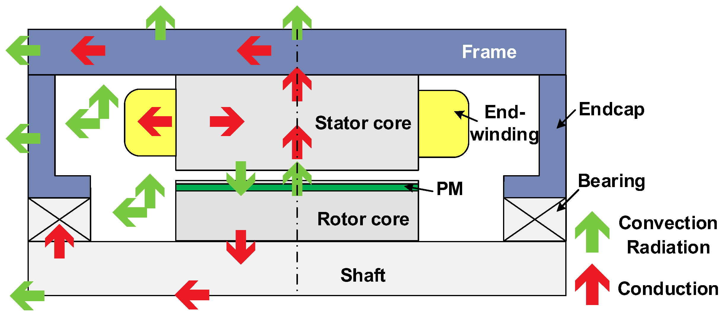
2. PM Machines and Heat Transfer Mechanisms

PM synchronous machines (PMSMs), as one of the most important brushless electrical machines, have been far more popular in various applications. For the common rotor PM machine, the rotor rotates synchronously with the stator armature reaction field and produces a constant rotor magnetic field by PMs. Thus, the torque can be produced by the interaction of the winding armature reaction and PM fields. The typical radial flux topologies, i.e., surface-mounted PM (SPM) and interior PM (IPM) machines, are illustrated in Figure 3.
Firstly, the SPM machine, as shown in Figure 3a, is the most widely used configuration due to its simple structure, where the PMs are mounted on the rotor surface and adjacent to the airgap. Since the relative permeability of PMs is almost the same as that of the air, there is negligible magnetic saliency and reluctance torque, and only PM torque is produced. For SPM machines, the PM eddy current loss could be significant since the PMs are directly exposed to the armature reaction field. Consequently, large eddy current loss will further increase PM temperature rise and demagnetization risk due to overheating.
Secondly, for the IPM machine, Figure 3b, PMs are embedded in the rotor core, and the leakage flux becomes more significant. Nevertheless, they have a high saliency ratio, i.e., the q-axis inductance is larger than the d-axis inductance, and thereby, they can utilize both PM and reluctance torques to significantly improve the ratio of resultant torque to PM volume. In other words, for the same output torque, the amount of PM materials can be reduced, which is an important advantage of IPM machines when expensive rare-earth magnets are employed. Meanwhile, IPM machines have a better flux-weakening ability and wider speed range since they generally have a higher d-axis inductance compared to that of the equivalent SPM machines. Meanwhile, the design of IPM machines is more flexible since there are more degrees of freedom, which further facilitates their applications. Although the PM loss in the IPM machine is generally lower than that in the SPM machine due to the shielding effect, the PM demagnetization caused by overheating is still a critical issue since the thermal condition on the rotor is usually poor.
In terms of driving currents, the PM machines can be divided into brushless alternating current (BLAC), also called PM synchronous machines (PMSM), and brushless direct current (BLDC) machines, whose back electromotive force (EMF) waveforms are sinusoidal and trapezoidal, respectively. Essentially, BLAC and BLDC machines should be driven under sinusoidal and rectangular phase currents, respectively. However, PM brushless machines may be operated in either BLAC and BLDC mode, although the efficiency, the torque ripple, and the thermal behaviours will be affected [6].
Within PM machines, the thermal energy can be transferred within solids or between the solid and the fluid. There are three types of heat transfer: conduction, convection, and radiation. Figure 4 gives an example of heat transfer paths in a natural cooling IPM machine.
Firstly, conduction heat transfer consists of the propagation of kinetic energy from warm molecules to cool molecules [88]. The conduction heat flux yields Fourier’s law (1), which states that “the heat flux resulting from thermal conduction is proportional to the magnitude of the temperature gradient and opposite to its sign” [89].
q con = λ T
where q con , λ , and T are the conduction heat flux density, the thermal conductivity, and the temperature gradient, respectively.
Secondly, the convection heat transfer is the macroscopic expression of the motion of the particles of the medium and yields Newton’s law of cooling [90], where the convection heat flux density q conv is defined as:
q conv = h c T T
where h c , T , and T are the convection heat transfer (CHT) coefficient, the body surface temperature, and the environment fluid temperature, respectively. In PM machines, the convection heat transfers occur within the airgap, the end-cap, between the housing and the environment. Moreover, the widely used cooling techniques, i.e., forced air- and liquid cooling, also mainly rely on enhancing convection heat transfer, which will be introduced in Section 4.
Thirdly, radiation heat transfer is an emission of electromagnetic waves from the objects having above zero absolute temperature. The radiative flux density q rad can be calculated as:
q rad = σ ε T 4 A
where σ   = 5.669 × 10⁻⁸ W/(m2K4) is the Stefan-Boltzmann constant. ε is the emissivity coefficient and depends on the surface material and finish [13,91]. T is the body absolute temperature in Kelvin. In addition, radiation heat transfer usually plays a minor role in electrical machines at normal ambient temperatures and is usually ignored or combined with convection heat transfer.

3. Machine Loss Estimation

During the energy conversion in PM machines, the loss generation is the inevitable parasitic effect, which is also the origin of temperature increases. The main PM machine losses include the stator and rotor iron losses, the copper loss, the PM eddy current loss, and the mechanical loss. The reliable loss estimation is fundamental for accurate thermal estimation. The various losses will be introduced below.

3.1. Stator and Rotor Iron Losses

Iron loss is one of the major losses in the PM machines, and the exploration of accurate iron loss prediction has over one-century history, which was firstly studied by C. Steinmetz [92] in 1892. The Steinmetz model can be written as:
P Fe = k f a B b
where P Fe is the iron loss, k , a , and b are Steinmetz coefficients.
With the improved understanding of iron loss, it was found that the generated iron loss can be separated from different origins, i.e., the hysteresis loss P hy , the classical eddy current loss P ec , and the excess loss P exc . To better reflect their different characteristics for engineering convenience, several iron loss models have been proposed and can be divided into two-term models [93,94,95] and three-term models [96,97]. Recently, it has been revealed in [98,99,100,101] that iron loss is also temperature-dependent.
Table 3 lists the common iron loss models, where k h and α are the hysteresis loss coefficients. k ec and k exc are the eddy current and excess loss coefficients, respectively. B m and f are the amplitude of the flux density and the electrical frequency, respectively. ϑ Fe . is the lamination temperature. In [97], σ , d , and T are the electrical conductivity, the thickness of the lamination, and the time period of the flux density waveform, respectively.
Furthermore, it is reported in [98] that by using the improved thermal-loss coupling method, i.e., considering the temperature dependency of iron loss, the temperature prediction accuracy can be significantly improved. However, it is worth mentioning that the temperature coefficients of hysteresis and eddy current iron losses depend on the flux density and electrical frequency, and thus they need to be determined based on extensive experiments. Moreover, the magnetic properties of silicon steel laminations are also affected by cutting and compression [102,103,104]. It has been demonstrated in the literature that both mechanical and laser cuttings could cause magnetic deterioration, and laser-cut materials have generally worse magnetic properties [102]. Consequently, it gives rise to higher iron loss. Furthermore, the compression of steel lamination caused by shrink fitting also causes a decrease in permeability and an increase in iron loss [104].

3.2. Copper Loss

Copper loss refers to the generated heat due to electrical resistance when the current flows through the wire. For coil-wound electrical machines, the copper loss is a large part of energy loss during the energy conversion, and can be divided into DC and AC components. The DC copper loss is calculated based on the DC resistance, while the AC copper loss is calculated accounting for the skin and proximity effects under the high frequency (HF) AC excitation. The skin and proximity effects represent the influences of the induced eddy currents on the distributions of current density for self-conductor and adjacent conductors, respectively [105]. The analytical calculation of proximity eddy current loss in the conductor can be found in [106,107,108]. Meanwhile, the large flux density variations near the stator slot opening for slotted machines could cause local concentration of AC copper loss for PMSM [109]. Thus, it is reported in [110] that an appropriate arrangement of conductors towards the bottom of the slot can reduce the AC copper loss. Furthermore, it is demonstrated in [88] that the current harmonics caused by the pulse-width modulation (PWM) effect will significantly increase AC copper loss.
Additionally, in comparison to the conventional stranded wire winding, the flat wire (hairpin) winding could increase the slot filling factor and reduce DC copper loss due to its larger cross-section, while the AC copper loss becomes more prominent due to the larger wire diameter [111]. In contrast, the Litz wire could restrain the skin and proximity effects and reduce the AC copper loss [112], while it could increase the DC copper loss due to its drawbacks of low package factor. Therefore, there is a trade-off between the DC and AC copper losses in the windings.

3.3. PM Eddy Current Loss

As is well known, a time-varying magnetic field could induce eddy currents. In an electrically conductive material, the induced eddy current will generate Joule loss. For PM machines during operation, the eddy current loss is generated by asynchronous airgap magnetic fields accounting for the influences of the non-sinusoidal stator winding MMF distribution [113,114], the slotting effect [115,116], the eddy current redistribution field [117,118], and the current harmonics caused by PWM [119,120,121].
Generally, the PM eddy current loss may be relatively smaller compared to the stator iron and copper losses. However, due to the poor thermal condition of the rotor, even a small amount of PM eddy current loss could cause local heat concentration. Meanwhile, as presented in Table 1, the NdFeB PM has a low electrical resistivity and further aggravates its thermal effect and the risk of demagnetization, particularly for the machines having high-speed, high pole number, large slot opening, and/or high power density.
In terms of calculation of PM eddy current loss, the FEM method is a common tool and exhibits a high estimation accuracy. To investigate the physical mechanism of eddy current loss, a huge number of papers regarding analytical calculation can be referred to, such as [116,117,118,119,120,121,122]. In general, the analytical calculation of PM eddy current loss aims to mathematically solve governing equations of magnetic and eddy current fields accounting for the slotting effect, the current harmonics, the eddy current redistribution field, etc. In addition, it is worth mentioning that the distribution of PM eddy current loss is usually non-uniform, which is mainly attributable to the slot opening effect and the armature reaction field. Consequently, the non-uniform loss distribution will give rise to the non-uniform PM temperature increases, and this increases the risk of partial demagnetization due to the hotspot. Detailed analyses of PM temperature distribution will be presented in Section 5.
In terms of reduction of PM eddy current loss, increasing the airgap length is the simplest way, since the high-order abundant field harmonics can be suppressed in the airgap. However, it is not practical for the PM machines requiring high torque density. Moreover, the common PM loss reduction methods include cutting off the complete eddy current paths by using PM axial/circumferential and even radial segmentations [123,124,125,126] or grooving the rotor sleeve [127], suppressing the penetration of MMF sub-harmonics by adding flux barriers on the rotor [128], as well as modifying airgap permeance by adding auxiliary slots from the stator side [129] or shaping the rotor surface [130]. However, there is a trade-off between the manufacturing difficulty and the PM loss reduction.

3.4. Mechancial Loss

Mechanical loss is a general term including windage loss and bearing friction loss. Firstly, windage loss refers to the air friction loss between the rotating rotor and the surrounding air. The windage loss is the energy loss during the acceleration of the surrounding fluid (air) and does not heat the machine but reduces the efficiency [37]. Since the windage loss depends on several factors, i.e., the physical properties of the fluid, the rotor speed, and the geometric parameters of the rotor, it could be more significant for high-speed and/or large volume PM machines.
In general, in electrical machines, the windage losses are generated in the tangential, radial and axial directions. Specifically, the tangential and radial windage losses occur in the airgap and the rotor end-surface due to the rotating rotor. The axial windage loss is generated due to additional forced axial fluid flow, e.g., caused by the axial fan cooling.
The windage losses are usually calculated by the empirical rules, which were developed in the last century and obtained by using the curve fitting technique based on the experiments for Ims. Indeed, they are also applicable for PM machines since the rotors in the PM machines can also be assumed to be a cylinder. The author in [131] summarises the existing empirical rules [132,133,134,135], which will be briefly reviewed below.
The tangential, radial, and axial windage losses P wind , δ , P wind , r , P wind , a are calculated as:
P wind , δ = k 1 C f , δ ρ f π ω 3 r o 4 l
P wind , r = 0.5 C f , r ρ f ω 3 r o 5 r i 5
P wind , a = k 2 q m ω r o 2
where k 1 is the roughness coefficient and equal to 1.0 for smooth surface and 2.5 for axial slotted surface [136]. C f , δ and C f , r are the tangential and radial friction coefficients, respectively. ρ f is the fluid density. ω is the rotor angular velocity. r o and r i are the cylinder outer and inner radii, respectively. l is the axial length. k 2 is the axial velocity factor and equal to 0.48 for smooth stator and rotor surfaces. q m is the mass of fluid flow rate within the airgap.
The friction coefficients C f , δ and C f , r depend on the cylinder outer radius and the Reynolds number ( R e ). R e is the ratio between the inertia and viscous forces and is used to determine the flow patterns of fluid flow, i.e., the laminar flow at low fluid velocity (small R e ) or turbulent flow at high fluid velocity (large R e ). In the tangential and radial directions, the types of fluid flow are determined by the Reynolds numbers R e δ and R e r .
R e δ = ρ f ω r o δ μ f
R e r = ρ f ω r o 2 μ f
where δ and μ f are the airgap length and the fluid dynamic viscosity, respectively.
Afterwards, the tangential and radial friction coefficients C f , δ and C f , r are determined as:
C f , δ = 0.515 ( δ / r o   ) 0.3 R e δ 0.5 500 < R e δ < 10 4 C f , δ = 0.0325 ( δ / r o   ) 0.3 R e δ 0.2 10 4 < R e δ                      
C f , r = 64 3 R e r                             R e r < 30 C f , r = 3.87 R e r 0.5                             30 < R e r < 3 × 10 5 C f , r = 0.146 R e r 0.2       3 × 10 5 < R e r
Secondly, the bearing friction loss P Bearing is a sum of rolling, sliding, seal, and drag losses, and is mainly dependent on the load and the rotor speed [137].
P Bearing = 1.05 × 10 4 M B × n
M B = 1 2 μ B P L d B
where M B and n are the frictional moment and the rotor speed, respectively. μ B , P L , and d B are the frictional coefficient, the load on the bearing, and the bore diameter, respectively. The frictional coefficient depends on types of bearing, e.g., μ B = 0.001 for a deep groove ball bearing. Meanwhile, the bearing friction loss could also be determined by the no-load deceleration tests and back-to-back drive tests [138,139].

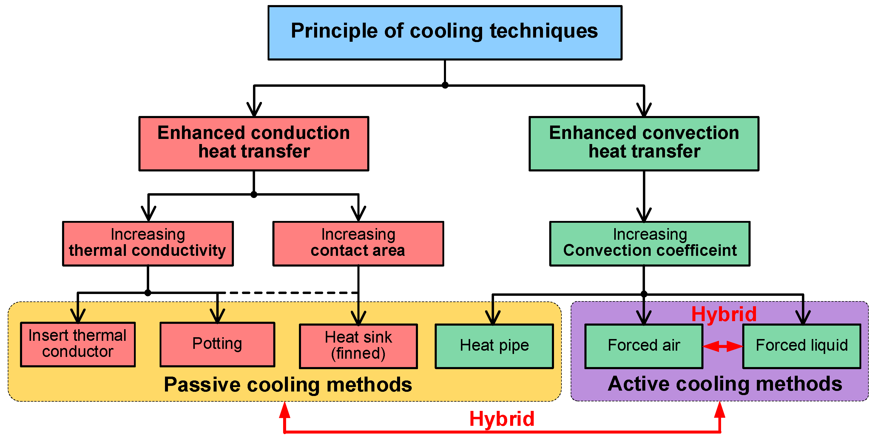
4. Cooling Techniques

The machine cooling technique is a straightforward way to increase the power density of PM machines by removing the generated heat. To date, various cooling techniques [140], including passive cooling, forced air cooling, and forced liquid cooling, have been developed based on the same principles, i.e., enhancement of either conduction or convection heat transfer, as illustrated in Figure 5. Meanwhile, different cooling methods can also be combined to further increase the machine cooling capacitance, which will also be reviewed in this section.

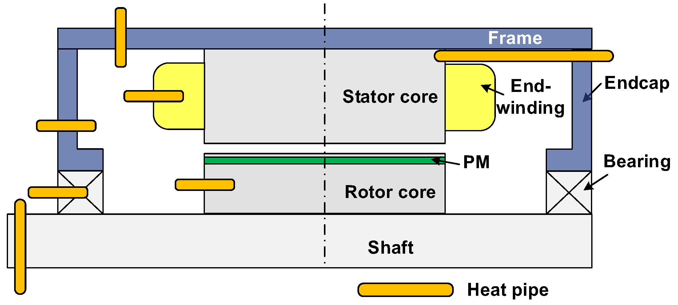
4.1. Passive Cooling

Passive natural cooling is the most common cooling approach for small- and medium-sized electrical machines, where the generated heat dissipates from the housing (frame and end-cap) to the environment via convection heat transfer. For instance, the heat transfer paths within an IPM machine have been shown in Figure 4. Nevertheless, in this case, the high temperature increases of coils and PMs under high power density are difficult to restrain.
Taking account into several practical factors such as cost, size, reliability, and construction complexity, the heat dissipation capability can still be enhanced in a passive way by enlarging the exposed surface of the housing (heat sink/finned housing) [141,142,143], guiding conduction heat transfer [144,145,146], or employing a heat pipe or potting [147,148,149,150].
Firstly, the finned frame in Figure 6 is a useful method to increase the outer surface area and/or the CHT coefficient [141]. It has been demonstrated in [142,143] that the thermal capacity of electrical machines can be improved by optimization of the geometric parameters and number of fins. Although the finned frame/heat sink could decrease the overall temperature levels of the machine, it only has a minor effect on the absolute temperature rises between the housing with the coils/PMs. Thus, its effectiveness in hotspot temperature reduction is limited.
Secondly, the thermal conductors could also be inserted into slots to guide conduction heat transfer from slot to housing (main heat removal path), and thus, restrain hotspot temperatures of active-winding. This is attributed to the higher thermal conductivity of inserted thermal conductors made of aluminium [144] or stator lamination [145] compared to the equivalent thermal conductivity of copper and insulation systems. However, besides the additional induced loss on the metallic conductors, it also brings difficulty in the winding process for a distributed winding configuration. Based on a similar working principle, both global winding [146] and end-winding [147] potting methods can mitigate high-temperature increases in the coils. Since the common potting material, i.e., resin, has a thermal conductivity of 1~3 W/m/K, it is still much higher than the air (0.02~0.03 W/m/K) within the end-cap. It has been demonstrated in the above literature that the hotspot temperature of end-winding can be effectively reduced.
Thirdly, the heat pipe utilizes the phase change of working fluid between the condenser and evaporator to absorb the generated heat. Due to its ultra-high thermal conductivity (>10, 000 W/m/K), a heat pipe has been widely used in different applications [32], including electrical machines [31]. The schematic diagram of various possible applications of heat pipes in electrical machines is shown in Figure 7 [31]. As observed, heat pipes can be assembled on the finned housing, the stator winding, the stator core, the bearing, the rotor, and the shaft. To date, the heat pipes buried in the active-/end-windings are more popular. This demonstrates that the heat pipes inserted in the active-winding [150] and in the end-winding [149] can lead to a 20% reduction of hotspot active-winding temperature and a 20 °C reduction of hotspot end-winding temperature, respectively. However, it needs to be emphasized that the heat dissipation capability of a heat pipe depends on its contact surface area, i.e., higher cooling effectiveness requires a larger contact area.

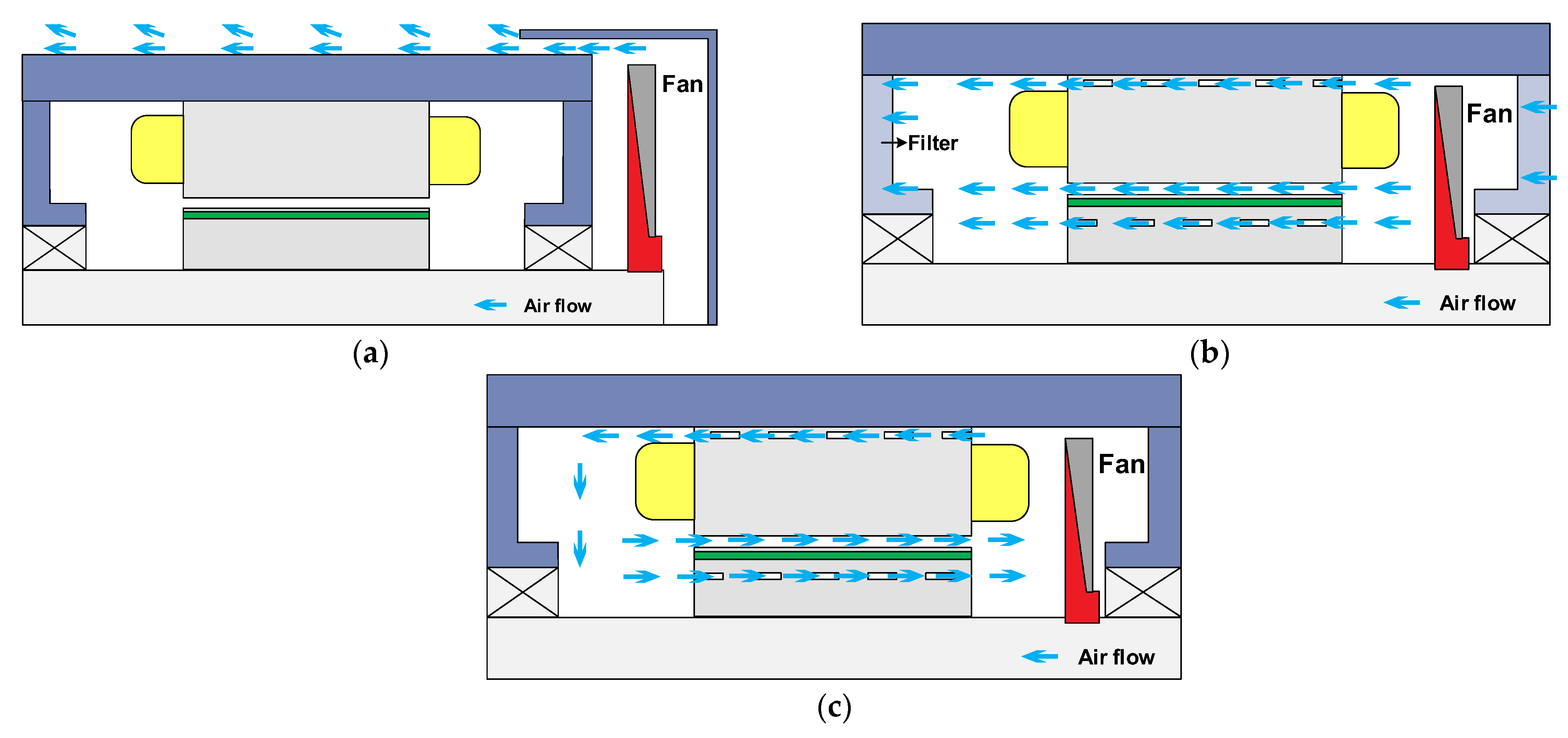
4.2. Forced Air Cooling

In comparison to passive natural cooling, the forced air cooling approach could increase the CHT coefficients not only around the frame but also within the machine. Normally, the fan is assembled coaxially with the shaft and enhances the fluid flow in the axial direction. The ventilation system can be classified as external fan cooling, internal open and closed fan cooling. Meanwhile, the external and internal (closed) fan cooling could also be employed simultaneously [22]. Figure 8 shows the air flows in different ventilation systems based on an IPM machine.
Firstly, for the external fan cooling in Figure 8a, the fan could accelerate the environmental air flow surrounding the electrical machine and enhance the forced convection heat transfer. The cooling effectiveness depends on the airflow rates, the shape and area of the housing, such as with a finned frame [151]. Secondly, for the internal fan cooling in Figure 8b, the fan could introduce cool air from the external environment into the machine from one side to the other side through filters on the end-plates [152], the airgap, or the stator and rotor ducts. Obviously, since the machine is exposed to the surrounding circumstances, dust, particles, and moisture may pollute electrical machines. Thirdly, to isolate the machine from the surrounding pollutants, the totally enclosed fan cooled (TEFC) ventilation system in Figure 8c is more popular and has been widely used [39,44,141,143,153].
Similarly, the enclosed fan cooling could accelerate the air flows within the machine, and the internal air circulates through stator and/or rotor ducts and the airgap. Furthermore, the circulated air flows could strengthen the heat dissipation from the machine to the environment through the housing. Compared to natural cooling, forced air cooling could reduce overall temperatures within the machine more effectively, while the high temperature rises of winding and PM may not be sufficiently restrained. Meanwhile, the assembled fan could cause additional loss, acoustic noises, and deconstruction risks, especially in high-speed applications.

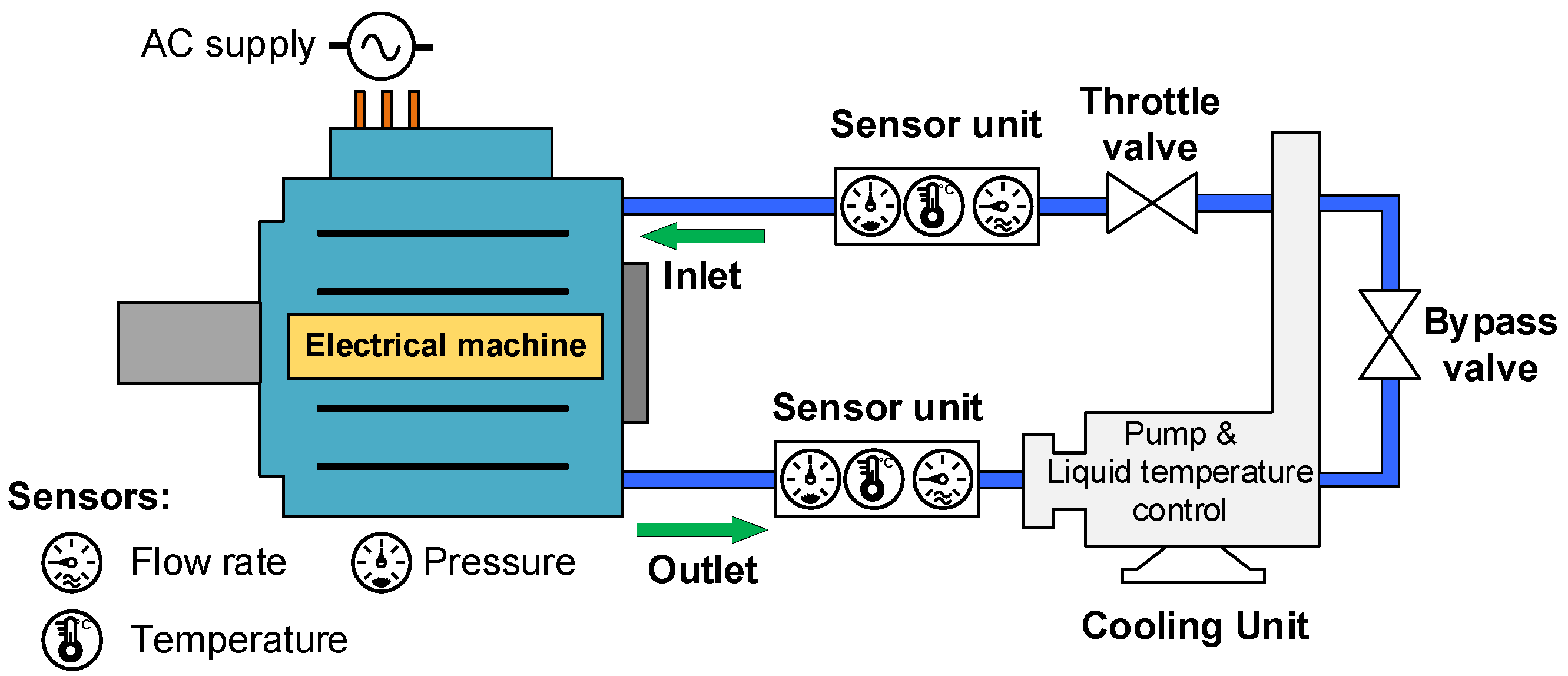
4.3. Forced Liquid Cooling

In high power applications, e.g., automotive traction machines, the forced liquid cooling technique is more popular due to its effectiveness [18,19]. Generally, compared to the forced air cooling method, the forced liquid cooling system requires additional apparatuses, e.g., high-pressure and scavenge pumps, liquid temperature control units, pressure and flow rate sensors, etc. In addition, the filter may be required when the oil is employed as the coolant. The schematic diagram of a forced liquid system is presented in Figure 9. As observed, the coolant flows from pumps into the electrical machine under high pressure at first. After flowing through the machine, the hotter coolant flows back to the pump. It is also worth mentioning that flow rate and the inlet coolant temperatures play a dominant role in the thermal management of the electrical machine. The flow rate is usually controlled by the throttle and/or bypass valves, while the coolant temperature could be cooled down by a radiator or condenser. In order to achieve satisfactory cooling effectiveness, turbulent flow is desired by increasing the flow rate. Meanwhile, the flow rate can be also adjusted according to the load conditions, especially under overload conditions.
According to whether there is a physical contact between the coolant and the machine components, in other words, whether the coolant needs to be sealed, forced liquid cooling can be divided into two types: the indirect and direct forced liquid cooling approaches. For indirect forced liquid cooling, the coolant does not directly contact the machine components and usually needs to be sealed. Otherwise, it is defined as direct forced liquid cooling in this paper.

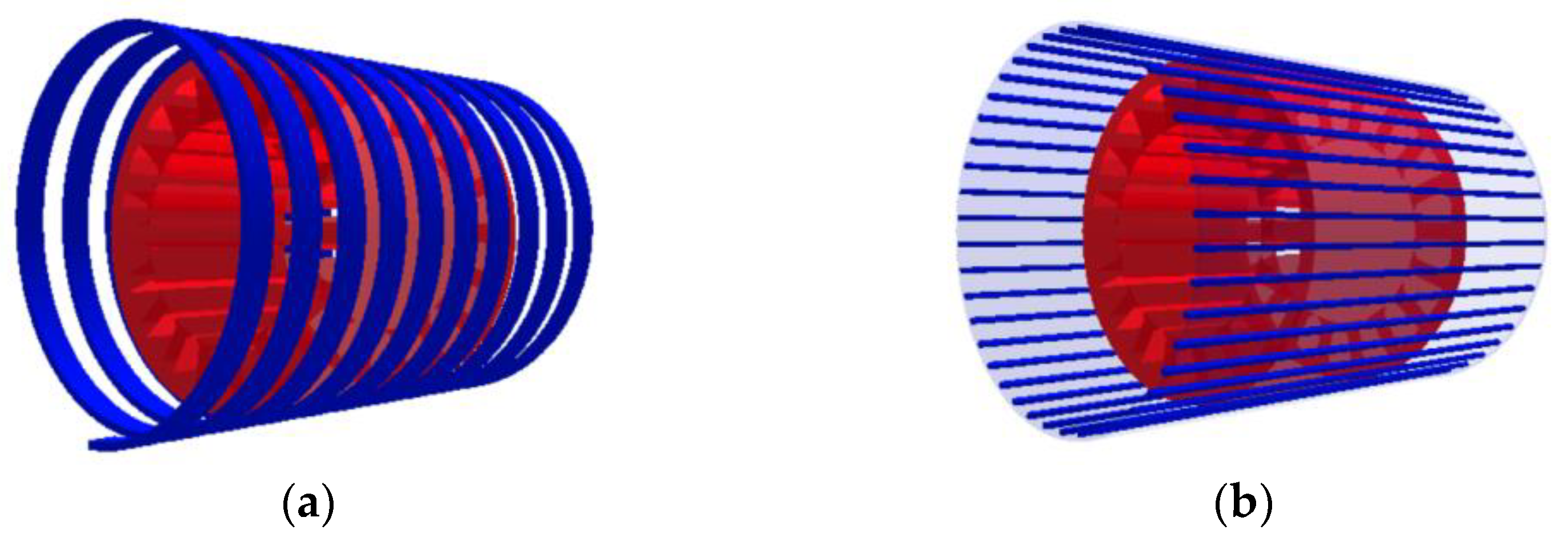
4.3.1. Indirect Forced Liquid Cooling

The indirect forced liquid cooling system mainly consists of cooling channels, coolants, and pumps. Firstly, the cooling channels can be grooved or installed within the frame [38,46,48,51,154,155,156], the stator core [157,158,159,160], the slot [161,162], the end-winding [163], and the shaft [164,165,166,167], as presented in Figure 10. Secondly, the liquid coolants could be water, ethylene glycol with water (EGW), or engine oil. Generally, water is preferred due to its high heat capacity. The potential leakage risk is the main issue.
The principle of forced liquid cooling is also based on the enhancement of convection heat transfer. In other words, the cooling capacity is affected by the CHT coefficients and the contact area. The CHT coefficients depend on the geometric parameters and shapes of cooling channels, the physical properties of coolant, and the flow rates [18]. The common frame liquid cooling channel configurations include spiral and axial [54], as shown in Figure 11. It has been reported in [167] that the spiral cooling channel could achieve higher cooling efficiency due to its lower fluid resistance, while the axial channel could achieve a higher contact surface. Similar to the forced air cooling, the frame and stator liquid cooling methods may be insufficient to restrain the hotspot temperature in windings and rotor PMs, which strongly depends on the coolant material, inlet temperature, flow rate, etc.
Furthermore, the cooling channels [161,162] installed in the slots in Figure 10c could significantly reduce winding temperature increases, but the slot filling factor will be sacrificed, and it is not easy to design a compact layout of cooling channels in the slots.
Additionally, the shaft liquid cooling system has been more popular recently, which is especially beneficial with regard to rotor PM temperature reduction [164,165,166], shown in Figure 10d. Meanwhile, it has been demonstrated in [166] that the liquid coolant tends to flow outwardly due to the centrifugal effect during rotation, which could further improve the heat dissipation capability. However, the construction of shaft liquid cooling is more complex, and the mechanical strength of the hollow shaft also needs to be taken into account. In [165], the common direct-through shaft liquid cooling [164,166], shown in Figure 12a, is compared with the recirculating shaft liquid cooling, as shown in Figure 12b. It is also reported in [165] that the recirculating shaft cooling has relatively higher friction loss but a higher CHT coefficient. However, as observed, the construction of the recirculating shaft liquid cooling is more complex.
The cooling channels can also be directly applied to the concentrated end-windings [163], as shown in Figure 10e, while the overhangs of end-winding would be longer than normal to leave the space for channels. It should be emphasised that for the indirect forced liquid cooling techniques, the risks of corrosion and liquid leakage should also be considered.

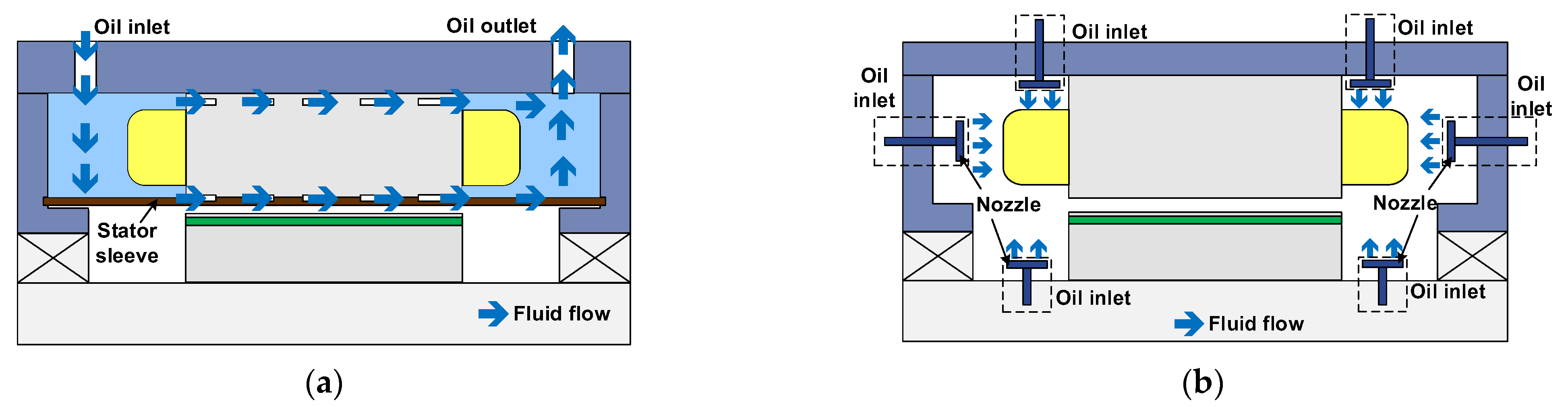
4.3.2. Direct Forced Liquid Cooling

The direct forced liquid cooling includes immersion cooling [168,169,170] and spray cooling [171,172,173,174,175], as presented in Figure 13. In comparison to indirect cooling, the coolant in a direct cooling system physically contacts specific components, i.e., end-winding and PM, and could provide a more effective temperature reduction due to shorter heat transfer paths.
For the stator immersion cooling in Figure 13a, its cooling principle utilizes high-thermal-conductivity oil to substitute the inner air within the stator part while increasing the CHT coefficient. In this case, the stator and the end-winding are immersed in the oil liquid. The oil could flow through stator ducts from one side to the other side and remove the heat from the stator core and the end-winding via convection heat transfer. However, it needs to be emphasised that the oil sleeve must be specifically designed to avoid oil leakage. In addition, the rotor can also be immersed in the oil liquid, which may lead to larger windage loss during rotor rotation due to the large fluid density of oil [169].
The spray cooling in Figure 13b has become more popular in recent years. An early study in [173] reports that spray cooling with refrigerant coolant provides a better cooling performance compared to immersion cooling. However, the proposed spray cooling is related to the phase change from liquid to gas. Thus, not only convection but also evaporation contributes to heat dissipation. In practice, spray evaporative cooling is still too complicated to be applied in the electrical machine due to the corrosion, pressure, environmental adaptation, compatibility and insulativity of coolants, as well as the additional condenser.
In contrast, spray oil cooling, which is pure convection heat exchange, is favourable due to its high stability and electrical insulation [174], and has also been employed in a Toyota Prius HEV in 2017 [172]. As can be seen from Figure 13b, the spray oil inlets could be located in the frame, the end-cap, or the shaft. The spray cooling is essentially based on the enhanced convection heat transfer between the sprayed cool oil with the end surfaces of end-winding and PM. In [173,175], the influences of oil flow rate, pressure, and the number of nozzles on the cooling efficiency, as well as the CHT coefficient, are investigated. However, it needs to be mentioned that the design of spray oil cooling is complex and exhibits large uncertainty, and the local hotspots in the end-winding may still exist. In general, the higher flow rate nozzles could achieve better cooling performance, while the additional power loss in the pump also needs to be considered. Meanwhile, since the coolant oil directly contacts the electrical insulation system, the long-term corrosion and material compatibility have attracted attention of late. It has been demonstrated in [176] that the different oil-based coolants significantly degrade the mechanical properties of wire coatings, which will also compromise the lifetime of electrical machines. As a summary, the features of different cooling techniques are evaluated in Table 4.

4.4. Hybrid Cooling

In some high-power density applications, a single cooling approach may be not enough. Hence, some combined cooling systems have been adopted simultaneously. The hybrid cooling methods can be performed by combining passive and active cooling approaches or by combining two active cooling approaches.
In terms of the combinations of passive and active cooling approaches, the finned frame with forced air cooling is one of the most common methods. In this case, the finned frame can increase not only the contact surface but also the turbulence of fluid, thus increasing the CHT coefficient as well [141,142,143]. Moreover, other passive cooling methods, e.g., additional thermal conductors in the slots, the potting, as well as the heat pipes, are also appropriately employed in forced air or liquid cooling systems [26], which could relatively restrain local overheating. However, it needs to be emphasised that the combined passive cooling components, i.e., inserted thermal conductors, heat pipes, and potting, should be physically connected with the main heat removal path to utilise their temperature difference.
In terms of combinations of the two active cooling approaches, they have been successfully applied to automotive traction machines, which are reviewed in [22,23,24] and are briefly listed below.
  • 2012 Tesla Roadster IM: inner forced air + finned housing + outer fan [22].
  • 2013 Tesla S60 IM: frame liquid + shaft cooling [24].
  • 2014 Porsche Panamera E-hybrid 416: frame liquid + forced air cooling [24].
  • GE IPMSM: frame liquid + end-winding spray + rotor cooling [177].
  • Zytek PMSM: frame liquid + forced fan cooling [178].
As can be easily found that the combinations of forced liquid and air cooling are widely used in automotive traction machines. However, other possible hybrid cooling methods are also worth further researching accounting for the specific thermal environments and applications. The thermal analysis of electrical machines under different cooling techniques can be implemented based on either LPTM or CFD. The LPTM relies on the CHT coefficients based on the empirical rules [23] and has the advantage of short computation time. However, regarding special and novel cooling systems, CFD and experiments are required to evaluate their cooling effectiveness and to calculate CHT coefficients. The detailed thermal analysis methods will be reviewed in the following section.

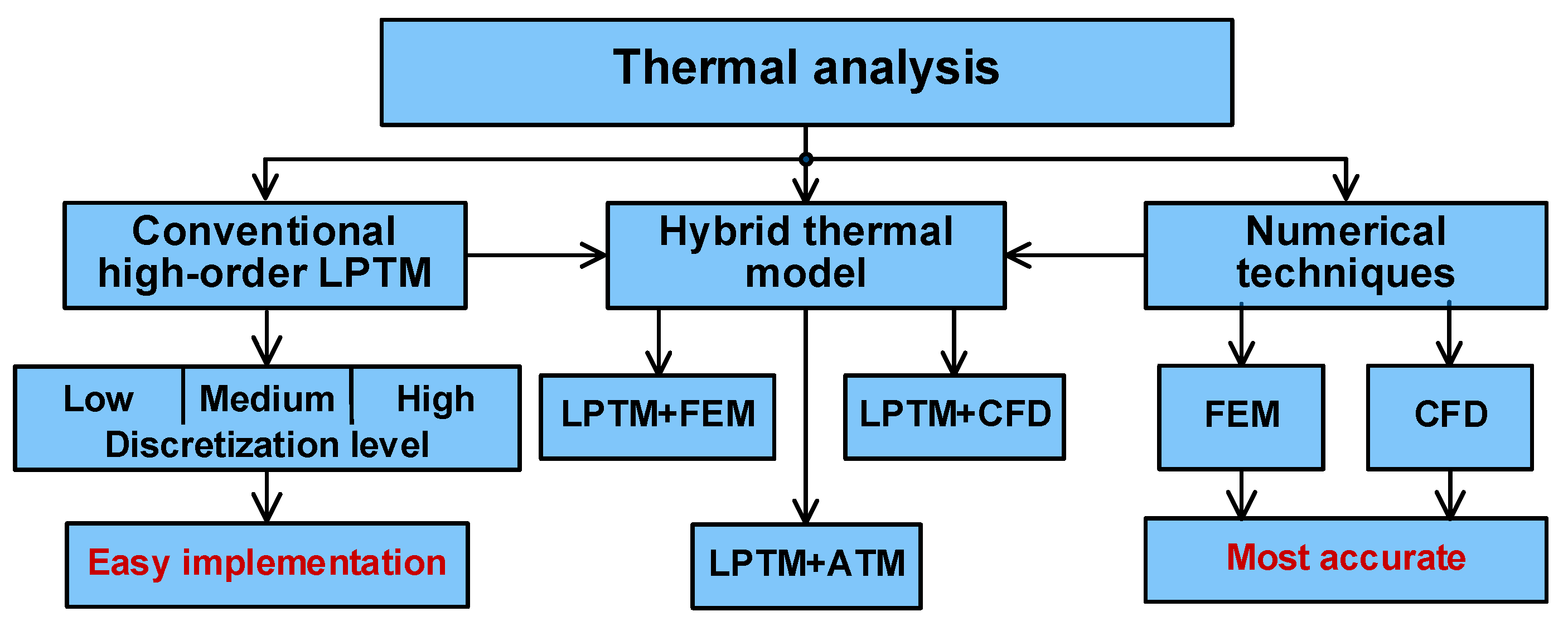
5. Thermal Analysis Methods

The thermal effect is one of the most critical factors to be considered at the machine design stage, and the machine designers usually restrict the current density according to the machine size based on previous experience [179,180]. However, it is a very rough indirect thermal analysis and may be not enough to prevent overheating.
Regarding the direct thermal analysis of electrical machines, there are two mainstreams: the numerical techniques, including FEM and CFD, and the conventional high-order LPTMs. Meanwhile, the hybrid thermal models, i.e., FEM + LPTM, CFD + LPTM, and ATM + LPTM, have become more popular in the last decade [181]. The main thermal analysis methods are summarized in Figure 14 and will be reviewed below.

5.1. Numerical Techniques

As is well known, the electromagnetic and thermal phenomena, as well as other most physical problems, could be described by a series of partial differential equations (PDEs), such as the Laplace equation, the Poisson equation, the wave equation, and the Fourier law. The PDEs can be solved by analytical or numerical methods. However, it is not always easy to find analytical solutions, especially for nonlinear problems with complex geometry. In contrast, the FEM becomes one of the most powerful tools for engineers in the fields of electromagnetics, thermodynamics, and fluid dynamics currently. Regarding the working principle of FEM, any large complicated system will be divided into large amounts of small meshed elements. By solving the PDE in every element numerically, a final solution can be obtained in FEM by combining approximated results in all elements.
As early as in the last century, the three-dimensional (3-D) FEM has been used to estimate the thermal behaviours for the turbine generator [182] and IMs [40,41]. In [42], a 3-D thermal FEM is developed to analyze the thermal fields of rotor conductor bars in the IM during starting. Furthermore, the axis-symmetric finite element model was developed in [43] to predict the stator and rotor winding temperatures for IMs under transient conditions. However, due to the limited computer competency, the FEM was mainly programmed manually based on the governing equations.
Since the 21st century, thermal FEM has been successfully included in the commercial electromagnetic analysis packages, including JMAG [183] and ANSYS [184]. Indeed, thermal FEM can accurately calculate conduction heat transfer with arbitrary geometric structures and provide detailed temperature distributions. Meanwhile, it can also be coupled with electromagnetic FEM considering non-uniform loss distributions.
Figure 15 gives examples of steady-state temperature distributions of a 12-slot/10-pole IPMSM calculated by 3-D ETFEM. To date, FEM methods have been extensively used for thermal analysis in PM machines, such as the BLDC machine [51], IPMSMs [46,185,186,187], axial flux PM machines [49,188,189,190], traction PM machines [154,191], and high speed PM machines [136,192,193,194].
On the other hand, the CFD is another numerical technique based on the finite volume method and primarily applied to estimate the fluid fields within and around the electrical machines, as well as the distributions of flow rate and pressure of the coolant in the cooling channels [13]. Before 2000, CFD was used to analyze the fluid field within the end-cap for TEFC IM, accounting for end-winding porosity [44] and geometric changes [45,195]. By using CFD software, the influence of shape of axial fan blade on the heat dissipation for IM is investigated in [196]. In [153], the temperatures for a TEFC IM predicted by the LPTM and the CFD are compared. This demonstrates that the LPTM could achieve high accuracy after thermal parameter tuning. Meanwhile, CFD is also used to estimate CHT coefficients within the end-cap [185,197,198] and the oil-based shaft cooling [164,165,166] for PM machines. It is also employed to estimate the fluid fields for the axial flux PM machines considering the fan cooling [188], the water-cooling [190], and the air-cooling [199] conditions. An example of the CFD simulation result of airflow velocity distribution within a fan-cooling PM machine is presented in Figure 16. In order to simulate the phenomena of turbulent fluid flow, the turbulent models include the one-equation Spalart-Allmaras model, the two-equation k-ε (kinetic energy- dissipation rate of turbulent kinetic energy) and the k–ω (kinetic energy- specific rate of turbulent dissipation) models. Generally, the computational burden increases rapidly with the equation numbers, while the convergence capability is also worse. However, the simple one-equation Spalart-Allmaras model is not appropriate for complex geometry since the turbulent scale is not taken into account in its one-equation governing equation. Therefore, two-equation turbulent models are more popular, where the k-ε model is a widely recognized industrial model and properly used to simulate the turbulent flow away from the wall [22]. In comparison, k–ω model is able to predict the viscous sub-layer and is more suitable for the separation flow perdition.
Overall, the FEM and CFD are useful numerical techniques to analyze conduction and convection heat transfer phenomena with complex geometric structures, respectively. However, they suffer from complicated model setup and extremely high computational burdens. More specifically, the thermal FEM and CFD always require a 3-D model [200,201], which severely increases computational time, especially in transient calculations [60]. Moreover, some components within the PM machines may be not critical in the electromagnetic FEM, e.g., the impregnation, the wire insulation, the slot wedge and liner, the bearing, the housing, etc., but they have a great influence on the thermal behaviours [17]. Consequently, the electromagnetic FEM usually cannot be directly used for thermal analysis. Sometimes, specific knowledge and experience are also required. In contrast, the conventional high-order LPTMs are more preferred due to their easy implementation and short computation time, which will be introduced below.

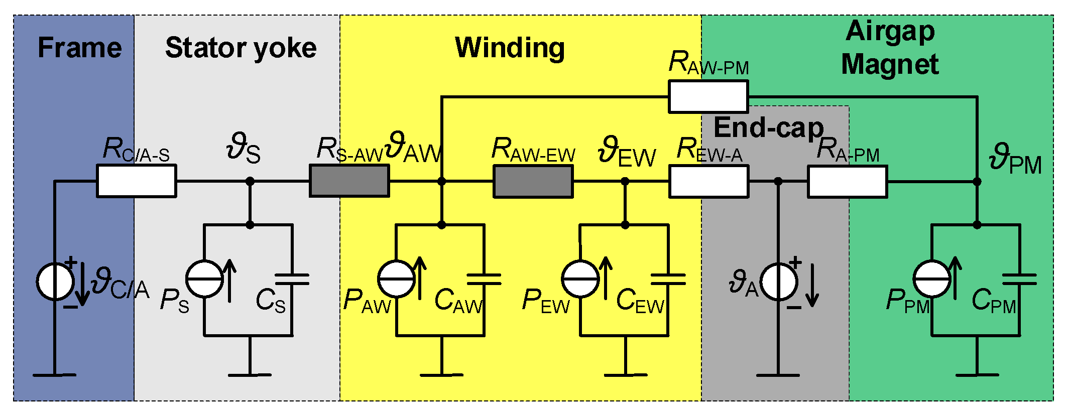
5.2. Conventional High-Order Lumped-Parameter Thermal Model

In the LPTM, the temperatures, the losses, the thermal capacitances and resistances correspond to the voltages, the currents, the electrical capacitances and resistances in the electrical circuit. The conduction, convection, and radiation heat transfers are represented by the respective thermal resistances, i.e., R cond , R conv , and R rad , which are expressed in (14)–(16), respectively.
In terms of conduction heat transfer within a solid, LPTMs are constituted by either “T-type” [34,60,61,62,63,156] or “I-type” [37,38,65,155] elementary conduction thermal networks, which are used to estimate average ϑ avg and mid-point ϑ mid temperatures, respectively. The one-dimensional (1-D) elementary thermal network in the x-direction is shown in Figure 17, where ϑ x , 1 , ϑ x , 2 , and P are the boundary conditions and the power loss, respectively. R x 1 , R x 2 , and R xm with/without superscripts are the conduction thermal resistances. C is the thermal capacitance, as expressed in (17), where c p and m are the specific heat capacity and the mass of the component, respectively.
R c o n d = L λ A
R c o n v = 1 h c A
R r a d = 1 h R A
C = c p m
In addition, for multiple-dimensional temperature calculation, the separate thermal networks in all directions are connected to the midpoint, where the heat fluxes in different directions are assumed to be independent. The 2-D or 3-D thermal modelling of each component depends on whether there is heat flow in the third direction. For instance, since there is no heat flow in the circumferential directions for a general cylinder, the 2-D thermal network in the radial-axial plane is appropriate [34]. However, for the thermal modelling of winding, 3-D thermal modelling is necessary since 3-D heat flows exist [202,203].
According to the discretization level, the conventional LPTMs for electrical machines can be classified as:
Firstly, in the discretized LPTMs, each component within the machine is discretized into several small networks. As an example, Figure 18 shows a 2-D “I-type” based discretized LPTM for a 15 kW TEFC IM [37], which is used to calculate the spatial temperatures for the main components.
Secondly, in the sophisticated LPTM, each component is individually modelled, while the less important component, e.g., rotor core, is lumped into one node to reduce the model complexity. However, for the component of greater thermal significance, e.g., winding, it will be modelled elaborately, e.g., by a 2-D multi-layer model [14,17,65] and a 3-D cylindrical segment [66]. Figure 19 shows a typical sophisticated LPTM built in the Motor-CAD [54] for a 12-slot/10-pole IPMSM [30].
Thirdly, in most cases, simplified LPTMs are more prevalent, where the components having indistinguishable thermal behaviours are merged into one node, such as end-cap and frame. The simplified LPTMs are firstly developed for IMs [34,37,39] and then applied to PMSMs [38,46,47,48,59,60,61,62,63,64,65,66,85,154], and stator PM machines [207,210],. The classical “T-type” and “I-type” based simplified LPTMs for PMSMs are presented in Figure 20.
As can be seen from Figure 18, Figure 19 and Figure 20, all main components within the PMSM need to be involved in any LPTMs to maintain the integrity of the entire thermal network. Meanwhile, the definitions of thermal resistances in (14)–(17) are valid for all LPTMs regardless of the level of discretization. Therefore, there is no substantial difference.
In terms of transient temperature calculation, the thermal network is described by the first-order ordinary differential equation system. In the discrete-time domain, it could be solved directly or approximately by using the well-known Runge-Kutta method [81,82,83,84]. Once the heat fluxes [154] or the temperature rises [155] between two iterative time steps approaches zero, it can be determined that the machine reaches thermal equilibrium.
The characteristics of “I-type” and “T-type” elementary thermal networks are summarized below. The following statements are also applicable to the complete LPTM constituted by the corresponding elementary thermal networks.
Firstly, it is obvious that the “I-type” elementary network has a simple structure to predict the midpoint temperature, while it is developed based on the assumption that the internal loss is generated concentratedly on the midpoint. However, in most cases, the internal loss is generated distributedly throughout the component. Consequently, the “I-type” based LPTM always overestimates the mid-point temperatures due to its concentrated loss input, and the estimation error is proportional to the ratio of the loss in thermal conductivity [211,212]. Thus, this issue is more serious for the active-/end-windings, since they always have low thermal conductivity (<1 W/(m⋅K)) and generate a large copper loss.
Secondly, the “T-type” introduces a negative compensation resistance in each direction to restrain overestimation of 1-D average temperature. However, the estimation performance could be deteriorated significantly in multiple dimensional thermal calculations, especially when the component has a large spatial temperature gradient. This is explained by the fact that in LPTMs, the heat flows are assumed to be independent in multiple dimensions, but the average and hotspot temperature strongly depend on the calculation dimensionality and temperature gradients.
Thirdly, and most importantly, the sophisticated and simplified “T-type” and “I-type” based LPTMs are incapable of estimating the hotspots. The local discretized LPTMs have been applied to assess the slot temperature distributions and hotspots considering the ac copper loss [204] and the back-iron extension [206], as shown in Figure 21. However, the employed “I-type” elementary networks also suffer from inherent defects. Consequently, a considerably large number of nodes (>100) is required to restrain the estimation errors [13,206], but it considerably increases computational burden and modelling difficulty, as shown in Figure 22. Thus, the LPTM loses its superiority of easy implementation.
In summary, sometimes the most concerned maximum temperature cannot be determined or determined accurately in conventional high-order LPTMs. Meanwhile, both the inappropriate calculation of convection coefficients and the misestimation drawbacks would reduce the estimation accuracy, and consequently, give designers the wrong information at the machine design stage. To address this issue, LPTMs have been combined with FEM, CFD, or ATM to utilize the strengths of LPTM and numerical/analytical methods simultaneously, which will be reviewed below.

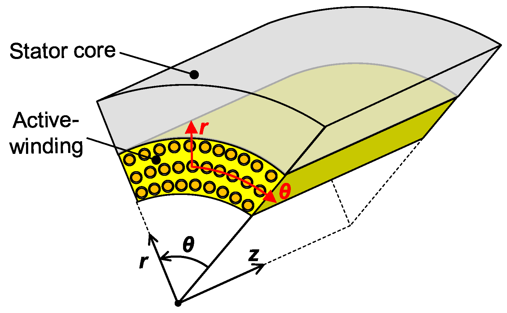
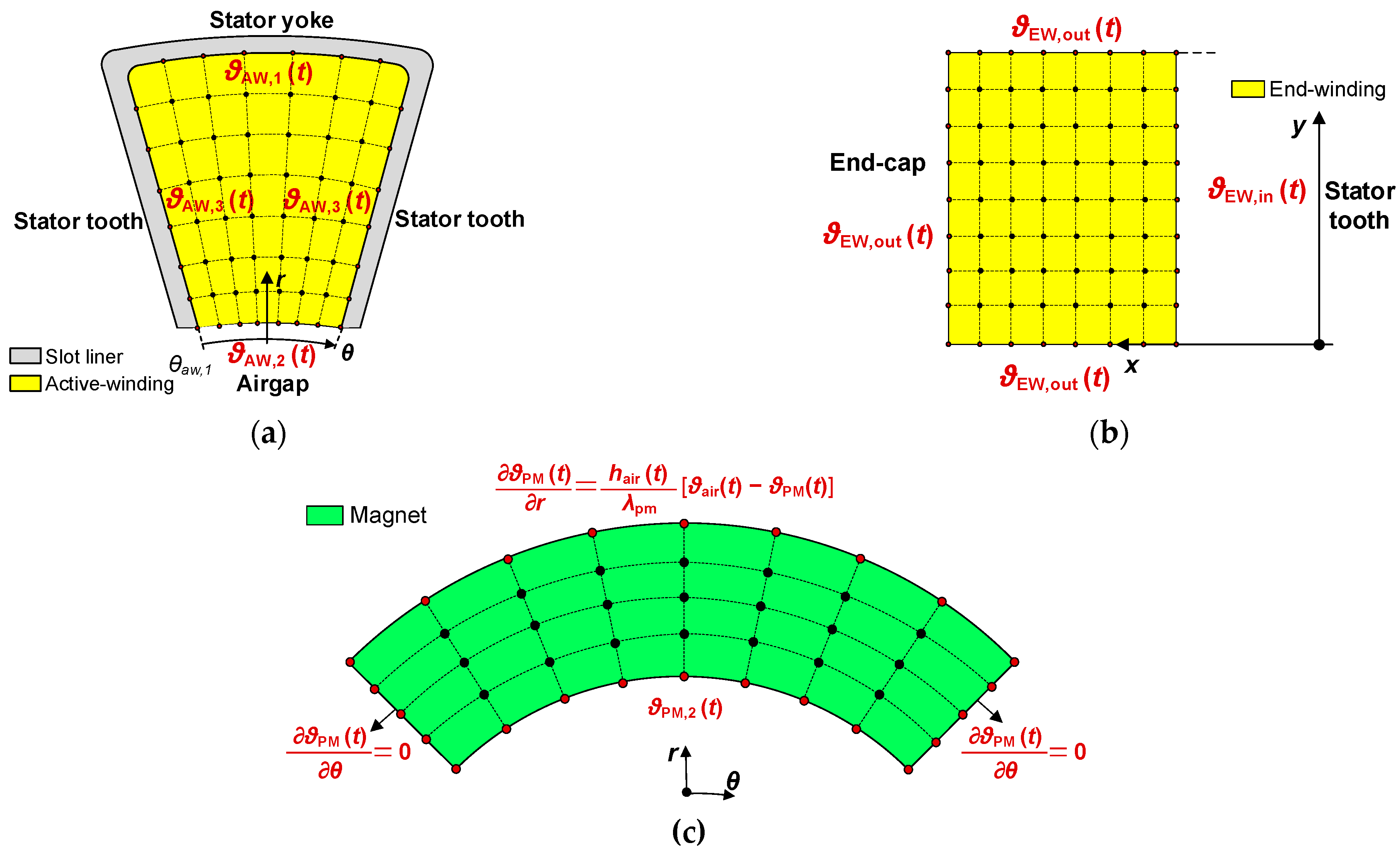
5.3. Hybrid Thermal Model and Analytical Thermal Modelling

As mentioned above, the hybrid thermal model utilizes the synergies of LPTM with partial CFD or with the FEM/ATM for different purposes. More specifically, regarding convection heat transfer, the partial CFD is used to calculate CHT coefficients for specific regions, which will be further used to determine convection thermal resistances in the LPTM. Meanwhile, regarding conduction heat transfer, the boundary temperatures calculated by LPTM can be employed into FEM or ATM to estimate the temperature distributions for the most important components. The concept and classification of the hybrid thermal models are presented in Figure 23.
The first hybrid thermal model is proposed in [37] and applied to a TEFC IM, where the LPTM and the analytical CFD are combined to calculate the conduction and convection heat transfers (within the end-cap). Furthermore, the partial CFD packages are adopted to estimate only the coolant distribution in the cooling channel and the fluid field within the end-cap for an IM under the steady [41] and transient states [42]. In comparison to the complete CFD modelled for the entire electrical machine, the partial CFD could significantly ease the computational burden [43]. Furthermore, the partial thermal FEM is used to estimate slot temperature distributions and determine the structure of a multi-layer active-winding LPTM for a PMaSynRM [44], where the boundary conditions are calculated by LPTM and then applied to the partial FEM.
In comparison to thermal FEM, the thermal analytical method is more preferable since it can be easily integrated with the LPTM and requires much less computation time with competitive estimation accuracy. Meanwhile, the thermal analytical method is also qualified to estimate temperature distributions and hotspots. This method has garnered much more attention in the last decade [181].
In the hybrid thermal model combining LPTM and ATM, similar to the LPTM+FEM, the boundary conditions are calculated by LPTM, and then they are applied to solve the conduction heat Equation (18).
c i ρ i ϑ i t = λ i 2 ϑ i + q i
where ϑ i and α i are the temperature and the thermal diffusivity of the solid component (i). 2 is the Laplace operator. q i is the loss density. c i is the specific heat capacity. ρ i is the mass density. λ i is the thermal conductivity. In addition, when the temporal derivative ϑ i / t equals zero, the conduction heat equation is used to calculate the steady-state temperature distribution.
For active-winding, a simple ATM is proposed in [64] to calculate the active-winding over-temperatures and the feasible current densities at the machine design stage, but the boundary conditions are not considered. In addition, similar to [64] in Figure 24, a circular multi-layered winding model combined with a 2-D active-winding ATM is proposed in [65]. To improve the estimation accuracy, the structure of multi-layered active-winding model is determined by the temperature gradients obtained from the ATM, and need to be “dynamically” adjusted according to different load conditions.
It is worth mentioning that in the multi-layered winding thermal model, either the elliptical multi-layers or the similar triangular multi-layers may suffer from an obvious drawback that the estimation accuracy is sensitive to the thicknesses of virtual impregnation layers due to its extremely low thermal conductivity, i.e., a slight structural change of the virtual impregnation layer will cause a large temperature variation. Consequently, it is challenging to determine an accurate multi-layer structure at the machine design stage due to lack of experimental results.
Both concentrated and distributed end-windings have disparate thermal conditions compared to the active-winding, since end-windings are usually exposed to the inner air within the end-cap. It has been demonstrated in [163] that the temperature of a concentrated end-winding is still ~20 °C higher than that of active-winding under a high-power supply. Therefore, two ATMs for active- and end-windings are modeled separately in [66], where an iterative adjusting process is also developed to overcome the misestimated average temperatures caused by the “T-type” elementary network.
Figure 25 shows an example of steady-state temperature distributions of active- and end-windings for a 12-slot/10-pole IPMSM with concentrated winding [66]. For the active-winding under the copper loss of 9.1 W per slot, the average temperature predicted by the “T-type” network equals 122.9 °C. It is ~5 °C lower than the hotspot temperature of 127.8 °C but is still 8 °C higher than the average temperatures of 115.0 °C calculated by FEM and ATM. The misestimation also occurs in the end-winding. More specifically, a comparison of temperatures predicted by the FEA, the LPTM, and the hybrid thermal model is listed in Table 5, where the detailed information refers to [66]. It can be easily determined that the exemplary results underpin the misestimation issues in conventional LPTM. In comparison, the hybrid thermal model has the similar accuracy compared to thermal FEA.
For PMs, the first hybrid thermal model, LPTM+ATM, is proposed in [59], where a 2-D PM ATM is proposed in the radial-axial plane to compensate for the axial heat flux of PMs. However, the proposed PM ATM cannot determine hotspots since it ignores the temperature distributions in the radial-circumferential plane, where the PM temperature also varies largely. Therefore, the proposed ATM is only validated by the FEM solved under the same governing equation, but may fail to be validated by the ETFEM. Hence, several improved 3-D ATMs have been developed recently, which can predict the steady-state and/or transient spatial PM temperature distributions for both SPMSM with/without rotor sleeve [60,61,62] and IPMSM [63]. Figure 26 shows the steady-state temperature distributions of SPM and IPM calculated by ATMs and 3-D ETFEA [60,63]. In addition, Table 6 compares the average and hotspot PM temperatures predicted by the FEA, the LPTM, and the hybrid thermal model, where the PM eddy current losses in one PM pole are 7.6 W and 5.1 W, respectively. As observed, the conventional LPTM fails to predict the hotspot temperatures, and the non-uniform distributions of PM eddy current loss also cannot be considered.
Moreover, accounting for the retaining rotor sleeve in high-speed SPM machines, the completed thermal modelling of the rotor is developed in [60], where the different sleeve materials, such as stainless steel or carbon fibre, are taken into account. Based on a 3-slot/2-pole high-speed BLDC machine, the steady-state rotor temperatures of one PM pole in the r-θ plane predicted by the hybrid thermal model and the 3-D ETFEA are shown in Figure 27.
In addition, it is worthy of note that the PM eddy current loss is distributed non-uniformly, which is affected by the slot opening effect, the slot-pole number combinations, and the armature reaction field. Thus, the appropriate mathematical modelling of PM loss is essential. Figure 28 presents the matrix-based post-processing of PM loss and the associated PM temperature estimation method developed in [61].
It can be found that the decrease of PM loss in the radial (r-) direction due to the skin effect is described by a first-order linear equation, while the heat transfer in the circumferential (θ-) direction is ignored due to the periodic symmetry. Furthermore, the standard method of predicting 3-D analytical PM temperature distribution utilizes the multi-slice method based on the axial-radial (z-r) plane [60,63]. The analytical temperature calculation in the 2-D z-r plane can also be degraded to the r-direction, while the axial heat transfer must be considered [62].
As above, there are some common conclusions drawn below.
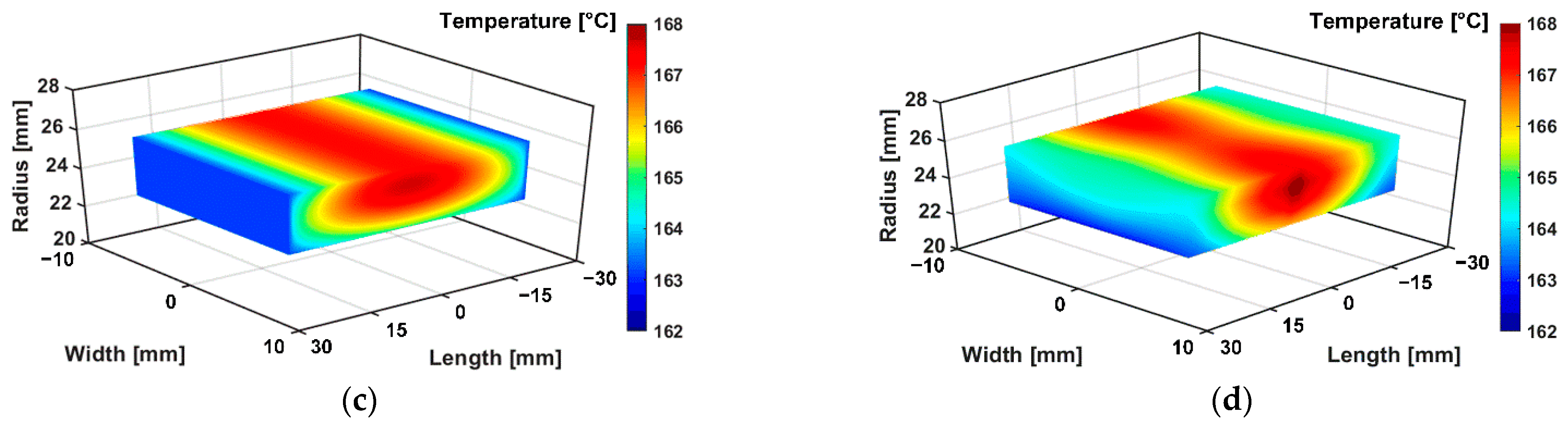
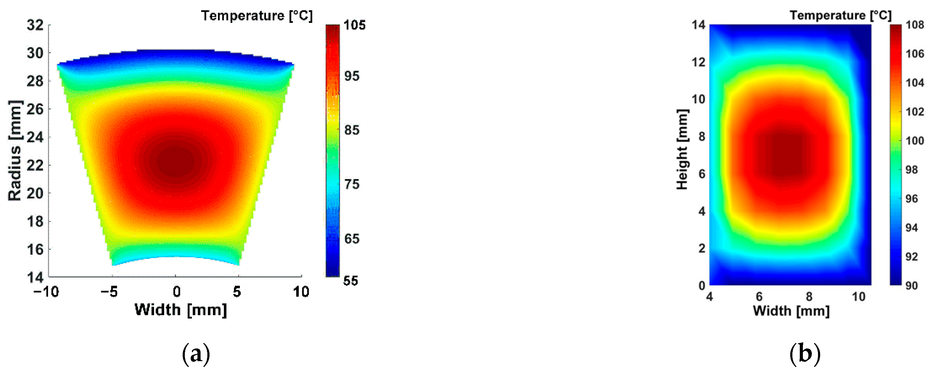
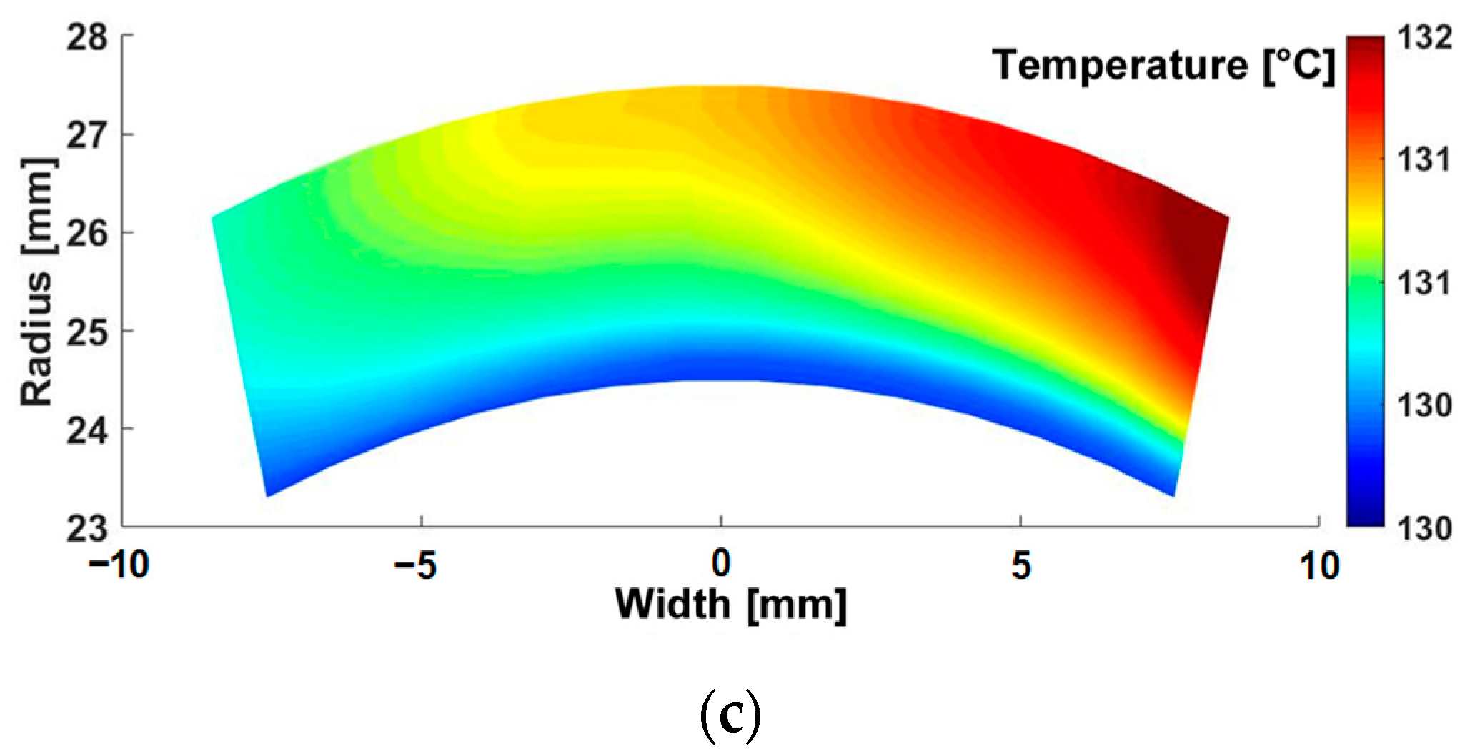
  • The PM temperature distributions and hotspots are strongly affected by the uneven distributions of PM eddy current loss and the boundary conditions.
  • The PM end-surface temperature is lower than the PM hotspot due to enhanced convection heat transfer.
  • The assumption of uniform PM eddy current loss distribution could cause severe misestimation of PM hotspots.
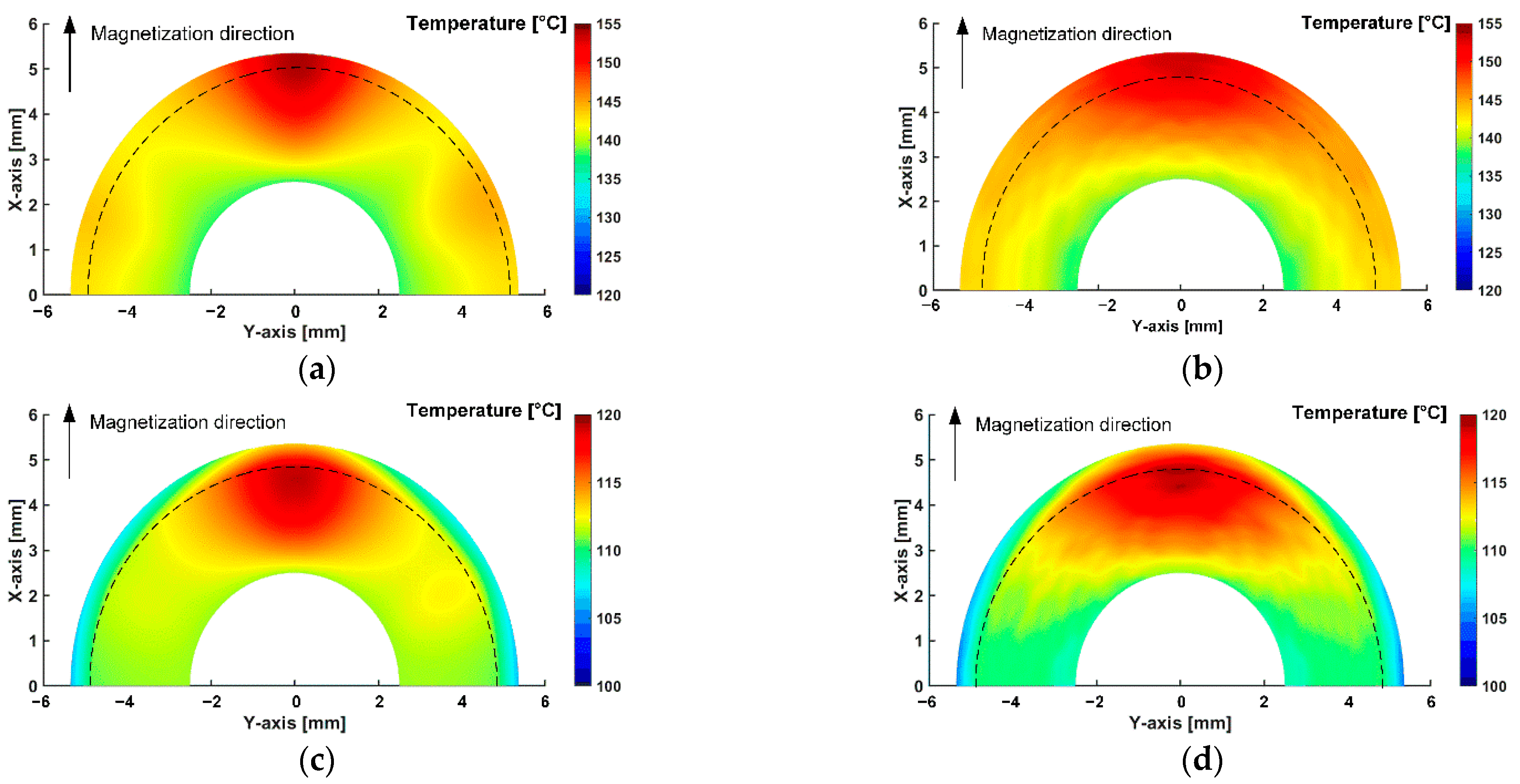
  • For the SPM, the PM loss can be dissipated to airgap via convection. Thus, the SPM hotspots are concentrated on the outer surfaces when the retaining rotor sleeve is not considered.
  • For IPM, the PM loss can only be dissipated to the rotor core via conduction. Consequently, the IPM hotspots occur in the upper part inside the PMs due to conduction heat transfer between the PM and the upper rotor core.
  • For SPM retained by a rotor sleeve, different sleeve materials have a significant impact on rotor thermal behaviors. Due to the low thermal conductivity of carbon fibre, the hotspot rotor temperature occurs on the adjacent interface between the PM and carbon fibre sleeve. In contrast, the metallic sleeve is beneficial for heat dissipation from the permanent magnet to the airgap. However, the additional eddy current loss induced on the metallic sleeve cannot be ignored.
In summary, Figure 29 summarises the hybrid thermal models and the analytical thermal models specifically for windings, SPM, and IPM, respectively, where the boundary conditions are also highlighted and tabulated in Table 7.

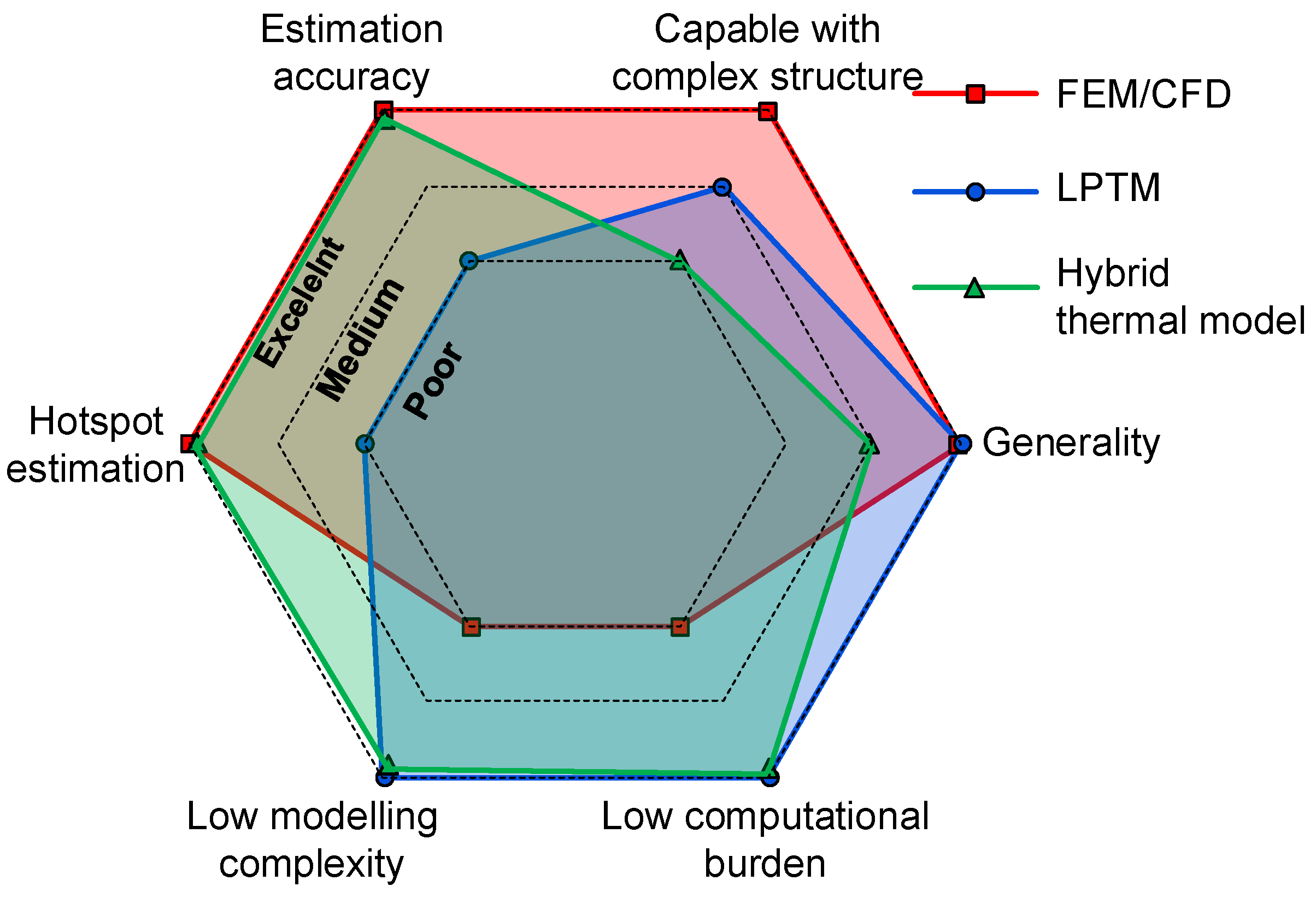
5.4. Evalaution and Assessment

Figure 30 and Table 8 demonstrate the features of the main thermal analysis methods. Indeed, the hybrid thermal model retains the merits of LPTM, i.e., low modelling complexity and computational burden, while also synergizing the strengths of FEM, such as being capable of predicting hotspots with high estimation accuracy. However, it needs to be emphasized that the ATM is mainly appropriate for the components having regular shapes. For example, if the PMs are shaped/grooved and/or have asymmetric geometry considering the minimization of loss [130] and torque ripple [213], numerical techniques are preferred.

5.5. Determination of Uncertain Thermal Parameters

Uncertainties of thermal parameters and properties are the other main challenges in thermal analysis and management. The critical thermal parameters include:
  • Material physical properties, including thermal conductivities, specific heat capacities, and mass density.
  • Contact thermal resistances of adjacent components caused by imperfect assembling, such as between the frame and the stator core, between the stator lamination and the winding, and between the shaft and the rotor core.
  • CHT coefficients within the machine under different cooling conditions.
Firstly, the physical properties of most materials can be found in the datasheet provided by the manufacturer or the data library in the FEA software. The main challenge lies in the modelling of winding, since it is constituted by multiple materials, i.e., the copper, the wire insulation, the impregnation, the slot liner, and/or the slot wedge. In practice, the winding is modelled as a composite solid instead of modelling for all individual wires. The composite solid of winding can be approximated by different models, such as a cylindrical rod [34], a rectangular shape model [37,38], two [39] or multiple layers [13,17,58], a cuboidal model [54], a cylindrical segment [202,203], etc. However, it is challenging to determine the equivalent thermal conductivity. From the perspective of heat transfer, the heat generated in the winding flows in three directions, the radial (r-), the circumferential (θ-), and the axial (z-) directions, as presented in Figure 31.
The radial and circumferential heat must flow through the wire insulation and the impregnation, which usually have extremely low thermal conductivities (<1 W/(m⋅K)). In contrast, the heat transfer along with the axial direction is much easier due to the high thermal conductivity of copper (~400 W/(m⋅K)). Hence, the composite solid has anisotropic thermal conductivities, and the low thermal conductivity in the r- and θ- directions are more critical since they can significantly increase winding temperatures.
Up to now, several approximations have been developed to determine equivalent thermal conductivities. In [34], a simple relationship between the equivalent thermal conductivity and insulation thermal conductivity is proposed. In [37], the Soderberg’s original expression [214] is rearranged and takes account into the effect of airspaces between the slot and the stator lamination. In [14,17], the winding is assumed to be modelled by two components, the inner copper and outer surrounding insulation components. Two regressive equations are developed to estimate the equivalent thermal conductivity of the outer insulation component based on a series of small- and medium-sized induction machines. In addition, the other widely used approximation is proposed by Hashin and Shtrikman (H+S) in [215], which can estimate the equivalent thermal conductivity accounting for two materials (copper and impregnation). More recently, an improved H+S approximation [216] is developed to calculate the composite thermal conductivity with three materials (copper, impregnation, and wire insulation). A summary is given in Table 9, where k f is the slot filling factor. λ in , λ imp , λ cu , and λ a are the thermal conductivities of the insulation, the impregnation, the copper, and the conductor together with the conductor insulation, respectively. A Slot and l aw are the slot area and the length of active-winding, respectively.
Secondly, in terms of manufacturing tolerances and surface roughness, the small airspaces caused by the imperfect assembling will significantly increase the temperature rise due to the extremely low thermal conductivity of air (~0.02 W/(m⋅K)). In practice, the airspaces are usually modelled by contact thermal resistances, and the exact values need to be determined based on a dc test by minimizing the predicted and measured temperatures [13,17,37,65].
Ultimately, for natural cooling, the CHT coefficient of the outer housing surface can be approximately equal to 5.95 W/(m2K) [14], which is assumed to be constant for most cases, since the variation of airflow velocity in the environment is usually ignored. For liquid cooling via cooling channels in the housing, the CHT coefficients depend on the shapes and geometric parameters of the channels, the flow rate, and the physical properties of the coolant [14]. Meanwhile, for unconventional cooling systems, e.g., the oil/water-based cooling via hollow shaft [166] and spray oil cooling [173,175], the CHT coefficients need to be determined by CFD software.
More recently, in [77,81], instead of using the empirical rules, the global parameter optimizations are carried out based on a set of comprehensive experiments to determine the thermal resistances and the convection coefficients simultaneously. However, the parameter identifications in [77] cannot reflect the thermal properties within the machine, since the identified LPTM is highly abstract. Meanwhile, the parameter identification in [81] is only concerned with the stator part under standstill with dc supply. Hence, global optimization provides a new perspective of thermal parameter determination and is worth further investigating, while a reliable and robust thermal model is required.

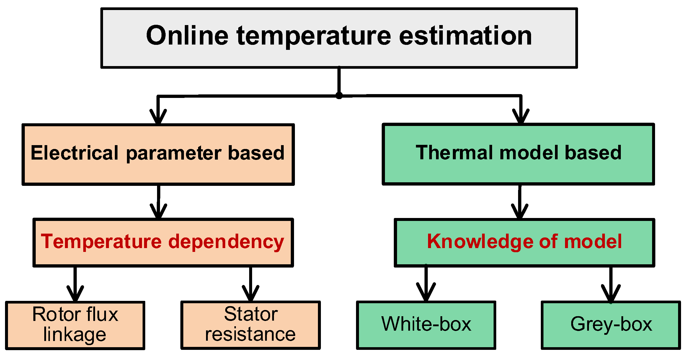
6. Online Temperature Estimation

In comparison to the thermal analysis at the machine design stage, the online temperature estimation during operation is equally or more critical. Normally, PMSMs are designed based on the demanding environment, including the highest ambient temperature, the insufficient cooling capability, and the heaviest load conditions. As a consequence, the machine usually operates with underutilized power since the actual temperatures are unknown.
Against this background, by measuring or estimating the most critical temperatures of windings and PMs, online thermal monitoring can significantly improve the utilization efficiency and prevent insulation failure and PM irreversible demagnetization caused by unexpected overheating. There are usually several thermocouples buried in the active-/end-windings during the winding process. However, the thermocouples increase the number of connections between the machine and the controller, which could reduce the system reliability and increase the complexity [217]. Meanwhile, the inserted thermal sensors may still be incapable of detecting the local hotspots.
On the other hand, it is challenging to assemble thermal sensors in the rotational rotor part during operation. The contact thermal sensors mounted in the rotor part rely on the slip ring, brushes, or hollow shaft for data transmission [218,219,220,221]. The non-contact infrared thermography relies on the visibility of the PM part [58,59,60,61,62,63,72,73,76]. Above all, both contact and non-contact measurement techniques are only appropriate in the laboratory environment and are not suitable in industrial applications since they give rise to additional costs, increase deconstruction risk, and/or are also difficult in terms of maintenance and replacement. Consequently, online temperature estimation methods have been widely investigated in the last decade and can be mainly categorized as the electrical parameter based methods [67,68,69,70,71,72,73,74,75,76,77] and the thermal model based methods [78,79,80,81,82,83,84,85], as shown in Figure 32 and reviewed as follows.

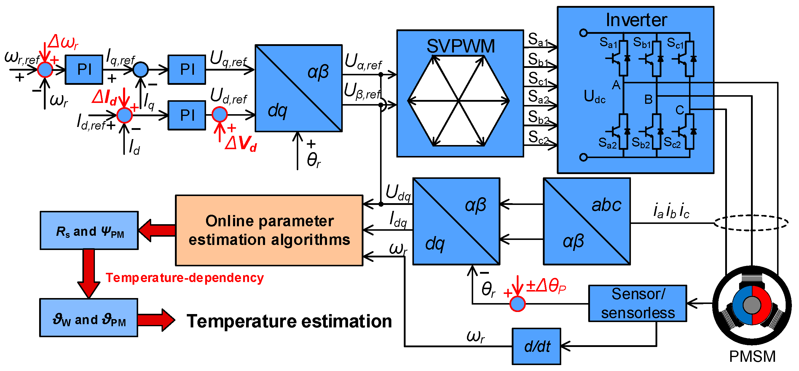
6.1. Electrical Parameter Based Methods

Generally, the electrical parameters, i.e., stator resistance R s and PM flux linkage ψ p m , are temperature-dependent (19), and thus, can be used as indicators to reflect average temperatures of winding and PM for online condition monitoring. Since the 2000s, the techniques of online parameter estimation for PM machines have been extensively investigated.
R s ϑ s = R s , 0 1 + α ϑ s ϑ 0
ψ p m ϑ p m = ψ p m , 0 1 + β ϑ p m ϑ 0
where α and β are the temperature coefficients of copper and PM, respectively. R s , 0 and ψ p m , 0 are the stator resistance and PM flux linkage at the reference temperature ϑ 0 . ϑ s and ϑ p m are the actual coil and PM temperatures, respectively.
In the online electrical parameter estimation, several critical issues need to be emphasized, i.e., the rank-deficient issue and the influence of voltage source inverter (VSI) nonlinearity. The detailed analyses can be found in [33,67]. This paper only gives a brief overview.
Firstly, as observed from the dq-axis steady-state voltage equation in (20), only two parameters can be estimated simultaneously based on one set of dq-axis voltage equations. If the number of unknown parameters is more than the rank of the system, the estimated results could not be converged to the correct values.
u d = R s ϑ s i d ω r L q i q   u q = R s ϑ s i q + ω r L d i d + ψ p m ϑ p m
where u d , u q are the dq-axis voltages. i d , i q are the dq-axis currents.   ω r is the electrical rotor speed. L d and L q are the dq-axis inductances.
On the one hand, some early papers regarding online parameter estimation suffer from the rank-deficiency, i.e., the estimated parameters could not be converged to the correct values [222]. On the other hand, some other papers fix several electrical parameters to estimate others [223], while the estimation accuracy may be deteriorated since both the magnetic saturation and the temperature effect will affect the electrical parameters. These papers will not be discussed.
Secondly, as one of the ill-conditioned issues, the VSI nonlinearity [224,225] severely affects the estimation accuracy of electrical parameters. The state-of-the-art online electrical parameter estimation methods are briefly outlined in Figure 33 and classified by whether magnetic saturation is considered [33].
In the last decade, the electrical parameter based temperature estimation has been extensively investigated. When the dq-axis inductances are known, the stator resistance and PM flux linkage can be estimated separately [69,75] or simultaneously [67,68] to monitor their thermal conditions, while the influences of magnetic saturation and nonlinearity of VSI should be considered. On the other hand, the signal injection methods are also popular, such as current/voltage injection [67,68,69], rotor position offset [70], variable rotor speed [71], and HF signal injection [72,73,74,75]. The schematic diagram of online parameter estimation is shown in Figure 34, where ω r is the variable of the rotor speed. I d and V d are the injected d-axis current and voltage.   ±   θ p are the injected position offsets.
The estimation algorithms include the Adaline neural network, the extended Kalman filter, the model reference adaptive system, the recursive least square, and the particle swarm optimization. It is worth mentioning that a reliable estimation model is the key point. If the estimation model is built appropriately, the different estimation algorithms may mainly affect the convergence speed but play a minor role in the identified values. A review of online parameter estimation and a detailed introduction of estimation algorithms can be found in [33].
Meanwhile, the HF signal injection methods have also been applied to estimate PM temperatures [72,73,74,75]. The HF voltage equations are expressed as:
u d hf r u q hf r = R d hf 0 0 R q hf i d hf r i q hf r + L d hf 0 0 L q hf d d t i d hf r i q hf r + 0 ω r L q hf ω r L dhf 0 i d hf r i q hf r
where u d hf r , u q hf r , i d hf r , and i q hf r are the dq-axis HF voltages and currents, respectively. R d hf , R q hf , L d hf , and L q hf are the dq-axis HF resistances and inductances, respectively.
The HF resistance R hf involves both the stator R shf and the rotor R rhf resistances, which are affected by the stator and rotor temperatures ϑ s and ϑ p m , respectively.
R hf = R shf ϑ s + R rhf ϑ p m = R shf , 0 1 + α ϑ s ϑ 0 + R rhf , 0 1 + β ϑ p m ϑ 0
where R shf , 0 and R rhf , 0 are the resistances at the reference temperature ϑ 0 .
Nevertheless, when R rhf is used to estimate PM temperatures [72,73], the varying PM magnetization state could cause the change of magnet resistivity due to the magnetoresistive effect, and thus, deteriorate the estimation accuracy. Secondly, L d hf is another indicator of PM temperature detection [75], since it is associated with the d-axis magnetic saturation and temperature-dependent magnet remanent flux. However, in this case, the information of self- and mutual-magnetic saturations on L d hf must be known in a prior. In addition, the HF injection-based PM temperature estimations have common drawbacks in that they are inapplicable at the high fundamental frequency, and they also introduce HF losses.
As a summary, the electrical parameter-based temperature estimations are easily integrated into the machine drive system and are capable of tracking the PM ageing effect. Nevertheless, they still suffer from some shortcomings.
Firstly, the temperature coefficients (absolute values) of the copper and the PM are considerably small at 0.39 %/°C and <0.2 %/°C, respectively. When the variations of stator resistance and the PM flux linkage are used to reflect their temperatures (19), the conversion coefficients equal the inverse of the small temperature coefficients. Therefore, the estimated temperatures are very sensitive to measurement errors, VSI nonlinearity, and parameter variations.
Secondly, even if the temperatures could be accurately estimated, they can only represent the average coil and PM temperatures, which may be much lower than the local hotspot temperatures, and thus the online electrical parameter estimation methods are not enough to prevent damages caused by local overheating.
Thirdly, the signal injection-based methods affect the stability of drive systems and could give rise to additional losses and disturbances.

6.2. Thermal Model Based Methods

In comparison, the thermal model-based method is the other mainstream method for online temperature estimation. The adopted thermal model can be classified as white-box and grey-box. In the white-box thermal model, similar to the conventional high-order LPTM, both the topology and the thermal parameters are known [47,63,85]. In contrast, in the grey box, the topology is usually constructed based on experience and knowledge of thermodynamics, while the thermal parameters are unknown and need to be identified [78,79,80,81,82,83,84,85].
Firstly, the thermal model-based temperature estimation should consider the following aspects.
  • Ability of predicting transient thermal behaviours.
  • Computation time and computing power of the processor.
  • Ability to track hotspots (desirable).

6.2.1. White-Box Based Thermal Model

Early in the 2010s, the high-order LPTM based real-time temperature estimation was reported in [47], as shown in Figure 35, where the thermal resistances and capacitances are calculated based on the heat transfer equations and empirical rules. The developed LPTM is represented as state-space equations and solved by using the Euler method for online implementation. However, the high-order LPTM still suffers from the misestimation issue and unknown hotspot, as discussed in Section 5.2.
Thus, more recently, the synergized thermal models [85], combining lumped-parameter and sub-domain thermal models (SDTM), have been developed for a 12-slot/10-pole fractional slot concentrated winding SPMSM in Figure 36, where the detailed machine parameters can be found in [85]. Afterwards, the SDTMs for the active- and end-windings and PM yield respective governing equations (18), and can be solved by utilizing the finite difference method. The interaction between the LPTM and SDTM, as well as the schematic diagrams of SDTMs, are presented in Figure 36c and Figure 37, respectively. The transient temperature distributions and hotspots for these vulnerable components are estimated numerically based on the information on transient boundary conditions. For instance, when the machine operates under 6.8 Nm at 600 r/min and 4.8 Nm at 7200 r/min with the ambient temperature of 20 °C, the corresponding predicted transient temperature distributions of winding and PM at 20 min are shown in Figure 38. It can be seen that the SDTM has a good prediction capability, especially in terms of critical hotspot temperatures.
As a summary, Table 10 compares the characteristics of ATM and SDTM. It can be easily found that their final solutions are the Fourier series multiplying exponential functions and the system of linear equations, respectively. However, there is no essential difference from the perspective of the concept. From this point of view, the analytical thermal models are equally appropriate under online conditions [63], while the analytical solution needs to be updated once the load condition is changed.

6.2.2. Grey-Box Based Thermal Model

However, the white box thermal model, Figure 35 and Figure 36, may be not appropriate in some low-cost applications due to the heavy computation burden caused by their high model order. To address this issue, some low-order grey-box thermal models have been developed subsequently [78,79,80,81,82,83,84] and then became the other popular method for online temperature estimation. In comparison, the low-order LPTMs only consider the most dominant heat transfer paths and the most important components, and thus, they only have two to five nodes to ease the computational burden. An improved low-order grey-box thermal model [84] is presented in Figure 39. It could predict the most critical temperatures of stator core ϑ S , the active-winding ϑ AW , the end-winding ϑ EW , and the PM ϑ PM . ϑ C and ϑ A are the reference temperatures the of coolant and ambient, respectively.
In general, the setup procedure of the grey-box thermal model is shown in Figure 40. Firstly, the constructed topology of the grey-box thermal model is essential for estimation accuracy and robustness, i.e., a slight inappropriate structural change would cause a large temperature error. Essentially, the grey-box thermal model should maintain the integrity of the entire heat transfer network of electrical machines to reflect the physical meaning. The inappropriate neglect of components and critical heat transfer paths could cause large estimation errors, especially when the grey-box thermal model is used beyond the training data domain. Furthermore, the redundant thermal resistances in the grey box thermal model could increase the computational burden during the parameter identification. Occasionally, some introduced virtual heat transfer path may negatively affect the model’s robustness.
Secondly, the thermal parameters in the grey-box thermal model are unknown since the heat transfer paths are highly abstract and/or the exact thermal properties or the geometric parameters are unknown. Thus, the thermal resistances are difficult to be calculated analytically in (14)–(17) but are usually identified based on the prior experiments (also known as the training domain). However, since some thermal parameters are varying with the rotor speed, the identification of thermal parameters in the PMSM belongs to a linear parameter varying system. The parameter identification of a linear parameter variation can be implemented by either local approach [78,79,80,81] or global approach [82,83,84].
In the local approach, the identification of a linear parameter varying system is divided into several linear time invariant sub-systems at different constant rotor speeds. For each linear time invariant sub-system, all thermal parameters are kept constant and associated with a constant rotor speed. Ultimately, regarding the entire speed range, all sets of linear time invariant sub-systems are saved into a look-up table. In the global approach, a comprehensive experiment is enough to identify all varying and constant thermal parameters. Thus, it is necessary to construct a mathematical function of varying thermal resistance with rotor speed. However, the highly abstract heat transfer paths would give rise to the difficulty in the construction of functions. Meanwhile, the low-order LPTMs also have drawbacks of the limited degree of freedom due to their abstraction. It has been reported in [84] that this drawback could be mitigated by introducing more degrees of freedom into the thermal resistance definition while not increasing the complexity of the model topology.
Ultimately, in terms of the estimation capability of the grey-box thermal model, after adequate data training, the improved grey-box model (see Figure 39) is employed to predict transient temperatures under two-hour varying load conditions based on a 12-slot/10-pole IPMSM (see Figure 40), as presented in Figure 41. It is obvious that the well-trained grey-box model could achieve an excellent estimation performance, and the maximum temperature errors are kept within 3 °C. However, it should be emphasised that the topology of the grey-box model must be robust, i.e., the abstract grey-box model is able to reflect the physical phenomena to the greatest extent. Meanwhile, the employed identification method also needs to be developed delicately.

6.3. Evaluation and Assessment

In comparison to electrical parameter-based temperature estimation, the thermal model-based methods are robust against measurement errors and parameter variations, and thus have a higher estimation accuracy. However, thermal model based methods require at least one sensor to provide the reference temperature since the temperature increases within the machine are relative values. More importantly, the white-box thermal models, Figure 35, Figure 36, Figure 37 and Figure 38, require accurate information on the geometric parameters and the thermal properties. Even though the exact machine information may be not necessary for the grey-box thermal model in Figure 39, the low-order grey-box thermal models have the drawback that they can only reflect the sensor measured temperatures. If the measured temperatures in the training domain are not the maximum temperatures, the identified model is also incapable of estimating hotspots. Table 11 summarises the advantages and disadvantages of main online temperature estimation methods.

7. Conclusions and Future Research Trends

With particular attention to the most critical hotspot temperatures, this paper reviews the development of thermal analysis and temperature estimation techniques over the last few decades. The state-of-the-art techniques are also evaluated and discussed. In addition, closely related machine loss estimations and cooling techniques are also outlined.
Currently, with the increasing attention to thermal analysis and thermal management of PM machines, the prospective research trends in this field could be initiated in terms of the following aspects:
1. 
Development of an accurate elementary thermal network.
As previously mentioned, the existing elementary conduction thermal networks more or less suffer from misestimation issues in the multiple-dimensional calculation. Thus, the further development of accurate elementary thermal networks is fundamental but could significantly reduce uncertainties in thermal analysis and temperature estimation.
2. 
Accurate identification of thermal parameters and properties.
The uncertainties of thermal parameters and properties severely affect the robustness and reliability of thermal analysis and temperature estimation. Thus, an accurate method of thermal parameter identification is valuable for both academics and industry.
3. 
Hotspot detection methods for different types of electrical machines.
So far, the recently developed hotspot detection methods are applied to the conventional radial-flux SPM and IPM machines. The specifical thermal modelling and hotspot estimation for other types of electrical machines are also valuable, such as axial flux PM machine, rotor wound synchronous machine, stator PM machine.
4. 
Investigation and application of advanced cooling techniques in different applications of PM machines.
The cooling technique is one of the straightest ways to improve the power density and operational reliability of PM machines. Meanwhile, in different applications accounting for machine configurations, operation conditions, and cost, the most appropriate cooling techniques, including hybrid cooling systems, are also worth investigating.
5. 
Systematic thermal analysis, modelling, and management of the integrated system of PM machine and inverter.
In some compact commercial products, the PM machine and inverter are usually integrated as a unit, and their thermal behaviours interact with each other. Thus, the complete thermal modelling and analysis for the integrated system are also important.

Author Contributions

Conceptualization, Z.-Q.Z. and D.L.; Methodology, Z.-Q.Z. and D.L.; Formal Analysis, D.L.; Investigation, D.L.; Resources, Z.-Q.Z.; Writing—Original Draft Preparation, D.L.; Writing—Review & Editing, Z.-Q.Z.; Supervision, Z.-Q.Z.; Project Administration, Z.-Q.Z.; Funding Acquisition, Z.-Q.Z. All authors have read and agreed to the published version of the manuscript.

Funding

This work was supported in part by the CRRC ZhuZhou Institute Co., Ltd., China, under Grant No. R/141597-12-1, Siemens Gamesa Renewable Energy A/S, Denmark, under Grant No. R/173973-11-1, the UK EPSRC Prosperity Partnership “A New Partnership in Offshore Wind” under Grant No. EP/R004900/1, and the UK EPSRC Future Electrical Machines Manufacturing Hub (EP/S018034/1).

Data Availability Statement

Not applicable.

Conflicts of Interest

The authors declare that they have no conflicts of interest. The funders had no role in the design of the study; in the collection, analyses, or interpretation of data, in the writing of the manuscript; or in the decision to publish the results.

Acronyms

ATMAnalytical thermal model
BLACBrushless alternating current
BLDCBrushless direct current
CFDComputational fluid dynamics
CHTConvection heat transfer
ETFEMElectromagnetic-thermal coupled FEM
FEM/AFinite element method/analysis
HFHigh frequency
IMInduction machines
IPMInterior permanent magnet
LPTMLumped-parameter thermal model
PMPermanent magnet
PMSMPermanent magnet synchronous machine
PWMPulse-width modulation
SPMSurface-mounted permanent magnet
SDTMSub-domain thermal model
SynRMSynchronous reluctance machine
TEFCTotally enclosed fan-cooled

Appendix A

Table A1 summarises some literature from 1990 to 2022, which is sorted by their published dates.
Table A1. Review of some thermal analysis literature for electrical machines.
Ref.MachineMethodologyCooling MethodRemark
FEACFDLPTM
1990s
[34,35,36,37,38,39]IM TEFCDetailed instruction of LPTM for IMs.
[40,41,42,43]IM TEFC2-D/3-D FEMs obtained by solving transient/steady-state governing equations.
[44,45,195]IM TEFCEstimation of fluid fields within the end-cap.
[131]IM Forced airMechanical loss estimation and thermal modelling based on LPTM.
2000s
[8]IM, SynRM FanThermal comparison of IM and SynRM.
[13]IM-Review of thermal analysis methods for electrical machine.
[14]Electrical machine Water/liquidReview of empirical rules of CHT coefficients.
[15]IM TEFCReview of CHT coefficients with the end-cap.
[16]PM machine Fan, naturalComparison of accuracy of CFD and Motor-CAD.
[17]IM-Review of thermal modelling of winding and CHT coefficients.
[38]SPM LiquidApplying LPTM from IM to PM machine for traction application.
[46]IPM machine WaterApplying LPTM [34] into IPM machine.
[49]Axial flux PM machine NaturalElectromagnetic, thermal, and fluid-dynamic analysis for axial flux PM machine.
[51]SPM machine, IM WaterInstruction of electromagnetic-thermal analysis of Motor-CAD.
[52]BLDC, SRM OilElectromagnetic and thermal analysis for BLDC and SRM for aerospace application.
[53]IM TEFCCombined CFD and LPTM for fast calculation.
[141]IMExperimentalFinned with fanEvaluation of heat transfer capability of a finned frame for different velocities of the cooling fan.
[153]IM TEFCComparison of estimation accuracy of temperatures predicted by CFD and LPTM.
[196]IM FanInvestigation of shapes of axial fan for open-type IM.
[211,212]Electrical machines -Improved 1-D “I-type” elementary thermal network to restrain temperature overestimation.
2010s to present
[22]PM machines Various cooling methodsReview of cooling methods for traction machines.
[30]PM machines Natural Review of empirical rules of CHT coefficients within PM machines.
[47]SPM machine NaturalReal-time implementation based on a conventional high-order LPTM.
[48]SPM machine WaterApplying LPTM [34] to a SPM machine considering driving cycle.
[55,56,57]PM machines Oil-, fan Combined partial CFD and LPTM to ease computational burden.
[58]PMaSynRM Water coolingCombined LPTM and partial FEM to estimate overall and slot temperatures.
[59]High-speed PM machines Natural, forced 2-D analytical PM thermal model to compensate for axial heat transfer in LPTM.
[60,61,63]SPMSM, IPMSM Natural Analytical thermal modelling of SPM and IPM machine based on a hybrid thermal model.
[62]High-speed PM machines Forced airAnalytical thermal multi-modelling of PM and rotor sleeve.
[58,65]IPM WaterMultilayer thermal modelling for winding based on FEA or analytical model.
[66]IPMSM NaturalHybrid thermal model predicting temperature distributions of active- and end-windings.
[81]PM machine Natural Thermal parameter tuning for stator part.
[85]SPMSM NaturalOnline tracking of hotspots of windings and PM based on the sub-domain thermal model
[86,87]PM machinesMachine learning-Neural network based black thermal modelling.
[136,192]High-speed PM machine FanLoss and thermal analysis for high-speed PM machines
[143]IM TEFC2-D analytical optimization of cooling fin for IMs
[154,191]IPM machines WaterElectromagnetic thermal analysis for traction IPMSMs
[162]PM machines WaterDeveloping a 3-D LPTM developed for hollow conductors with direct cooling
[164,165,166] PM machine Oil-based shaft coolingDetermination of convection coefficient of oil-based hollow shaft via CFD
[185]IPM machine Water Developing a full CFD model for IPM machine considering different rotor blade shapes
[186]PMaSynRM Natural Comprehensive analysis of PMaSynRM for traction application accounting for drive system
[187]PMaSynRM Oil Developing LPTMs for triple 9-phase PMaSynRM under various fault conditions
[188]Axial flux PM machines Fan Investigation of different fan blade designs for rotor cooling of axial flux PM machines by CFD
[190]Axial flux PM machine Water Grooving water-cooling jackets in the housing
[196]PM machine Natural Determination of convection coefficients within the end-cap
[199]Disc-type PM machine Forced airDetermination of convection coefficient by CFD
[204]IPM machine Natural A local discretized slot LPTM modelled to investigate the AC copper loss effect
[206]PM machine Water A local discretized slot LPTM modelled to investigate the back-iron extension effect
[207]Flux-switching PM machine Water FEM and LPTM modelling for flux-switching PM machines
[208]SPM machineNatural Optimization of SPM machine accounting for electromagnetic, vibratory, and thermal behaviour
[210]Flux-switching PM machine Natural Thermal–electromagnetic analysis for flux-switching PM machine considering driving cycle
[202,203]Basic element -Analytical derivations of 3-D “T-type” thermal networks for cubic and cylindrical elements.

References

  1. Waide, P.; Brunner, C. Energy-Efficiency Policy Opportunities for Electric Motor-Driven Systems; International Energy Agency: Paris, France, 2011; Available online: https://www.iea.org/reports/energy-efficiency-policy-opportunities-for-electric-motor-driven-systems (accessed on 1 May 2011).
  2. Rahman, M.A. History of interior permanent magnet motors [History]. IEEE Ind. Appl. Mag. 2013, 19, 10–15. [Google Scholar] [CrossRef]
  3. Cao, W.; Mecrow, B.C.; Atkinson, G.J.; Bennett, J.W.; Atkinson, D.J. Overview of electric motor technologies used for more electric aircraft (MEA). IEEE Trans. Ind. Electron. 2012, 59, 3523–3531. [Google Scholar]
  4. Chi, S.; Zhang, Z.; Xu, L. Sliding-mode sensorless control of direct-drive PM synchronous motors for washing machine applications. IEEE Trans. Ind. Appl. 2009, 45, 582–590. [Google Scholar] [CrossRef]
  5. He, T.; Zhu, Z.Q.; Eastham, F.; Wang, Y.; Bin, H.; Wu, D.; Gong, L.; Chen, J.T. Permanent magnet machines for high-speed applications. World Electr. Veh. J. 2022, 13, 18. [Google Scholar] [CrossRef]
  6. Zhu, Z.Q.; Howe, D. Electrical machines and drives for electric, hybrid, and fuel cell vehicles. Proc. of IEEE 2007, 95, 746–765. [Google Scholar] [CrossRef]
  7. Polinder, H.; Ferreira, J.A.; Jensen, B.B.; Abrahamsen, A.B.; Atallah, K.; McMahon, R.A. Trends in wind turbine generator systems. IEEE J. Emerg. Sel. Top. Power Electron. 2013, 1, 174–185. [Google Scholar] [CrossRef]
  8. Boglietti, A.; Cavagnino, A.; Pastorelli, M.; Staton, D.; Vagati, A. Thermal analysis of induction and synchronous reluctance motors. IEEE Trans. Ind. Appl. 2006, 42, 675–680. [Google Scholar] [CrossRef] [Green Version]
  9. National Electrical Manufacturers Association. Motors and Generators. Available online: https://www.nema.org/Standards/view/Motors-and-Generators (accessed on 1 December 2021).
  10. Gao, Z.; Cecati, C.; Ding, S. A survey of fault diagnosis and fault-tolerant techniques—Part I: Fault diagnosis with model-based and signal-based approaches. IEEE Trans. Ind. Electron. 2015, 62, 3757–3767. [Google Scholar] [CrossRef] [Green Version]
  11. Gao, Z.; Cecati, C.; Ding, S. A survey of fault diagnosis and fault-tolerant techniques—Part II: Fault diagnosis with knowledge-based and hybrid/active approaches. IEEE Trans. Ind. Electron. 2015, 62, 3768–3774. [Google Scholar]
  12. Liu, S.; Kuhl, G. Temperature coefficients of rare earth permanent magnets. IEEE Trans. Magn. 1999, 35, 3271–3273. [Google Scholar] [CrossRef]
  13. Boglietti, A.; Cavagnino, A.; Staton, D.; Shanel, M.; Mueller, M.; Mejuto, C. Evolution and modern approaches for thermal analysis of electrical machines. IEEE Trans. Ind. Electron. 2009, 56, 871–882. [Google Scholar] [CrossRef] [Green Version]
  14. Boglietti, A.; Cavagnino, A.; Staton, D. Determination of critical parameters in electrical machine thermal models. IEEE Trans. Ind. Appl. 2008, 44, 1150–1159. [Google Scholar] [CrossRef]
  15. Boglietti, A.; Cavagnino, A. Analysis of the endwinding cooling effects in TEFC induction motors. IEEE Trans. Ind. Appl. 2007, 43, 1214–1222. [Google Scholar] [CrossRef] [Green Version]
  16. Staton, D.; Pickering, S.J.; Lampard, D. Recent advancement in the thermal design of electric motors. In Proceedings of the SMMA Fall Technical Conference, Durham, NC, USA, 3–5 October 2001; pp. 1–11. [Google Scholar]
  17. Staton, D.; Boglietti, A.; Cavagnino, A. Solving the more difficult aspects of electric motor thermal analysis in small and medium size industrial induction motors. IEEE Trans. Energy Convers. 2005, 20, 620–628. [Google Scholar] [CrossRef] [Green Version]
  18. Staton, D.; Cavagnino, A. Convection heat transfer and flow calculations suitable for electric machines thermal models. IEEE Trans. Ind. Electron. 2008, 55, 3509–3516. [Google Scholar] [CrossRef] [Green Version]
  19. Taras, P.; Nilifard, R.; Zhu, Z.Q.; Azar, Z. Cooling techniques in direct-drive generators for wind power application. Energies 2022, 15, 5986. [Google Scholar] [CrossRef]
  20. Dong, C.; Qian, Y.; Zhang, Y.; Zhuge, W. A review of thermal designs for improving power density in electrical machines. IEEE Trans. Transp. Electr. 2020, 6, 1386–1400. [Google Scholar] [CrossRef]
  21. Deisenroth, D.C.; Ohadi, M. Thermal management of high-power density electric motors for electrification of aviation and beyond. Energies 2019, 12, 3594. [Google Scholar] [CrossRef] [Green Version]
  22. Gai, Y.; Kimiabeigi, M.; Chuan Chong, Y.; Widmer, J.; Deng, X.; Popescu, M.; Goss, J.; Staton, D.; Steven, A. Cooling of automotive traction motors: Schemes, examples, and computation methods. IEEE Trans. Ind. Electron. 2019, 66, 1681–1692. [Google Scholar] [CrossRef] [Green Version]
  23. Gronwald, P.; Kern, T. Traction motor cooling systems: A literature review and comparative study. IEEE Trans. Transp. Electr. 2021, 7, 2892–2913. [Google Scholar] [CrossRef]
  24. Popescu, M.; Staton, D.; Boglietti, A.; Cavagnino, A.; Hawkins, D.; Goss, J. Modern heat extraction systems for power traction machines—A review. IEEE Trans. Ind. Appl. 2016, 52, 2167–2175. [Google Scholar] [CrossRef]
  25. Wallscheid, O. Thermal monitoring of electric motors: State-of-the-art review and future challenges. IEEE Open J. Ind. Appl. 2021, 2, 204–223. [Google Scholar] [CrossRef]
  26. Zhu, T.; Zhang, Y.; Li, Q.; Wang, Y.; Geng, W. Overview of hybrid cooling system for high power density motor. J. Electr. Eng. 2022, 23, 1–16. [Google Scholar]
  27. Wang, Q.; Wu, Y.; Niu, S.; Zhao, X. Advances in thermal management technologies of electrical machines. Energies 2022, 15, 3249. [Google Scholar] [CrossRef]
  28. Ghahfarokhi, P.; Podgornovs, A.; Kallaste, A.; Cardoso, A.; Belahcen, A.; Vaimann, T.; Tiismus, H.; Asad, B. Opportunities and challenges of utilizing additive manufacturing approaches in thermal management of electrical machines. IEEE Access 2021, 9, 36368–36381. [Google Scholar] [CrossRef]
  29. Kulan, M.; Sahin, S.; Baker, N. An overview of modern thermo-conductive materials for heat extraction in electrical machines. IEEE Access 2020, 8, 212114–212129. [Google Scholar] [CrossRef]
  30. Liang, D.; Zhu, Z.Q.; Feng, J.; Guo, S.; Li, Y.; Wu, J.; Zhao, A. Influence of critical parameters in lumped-parameter thermal models for electrical machines. In Proceedings of the 2019 22nd International Conference on Electrical Machines and Systems, Harbin, China, 11–14 August 2019; pp. 1–6. [Google Scholar]
  31. Bradford, M. The application of heat pipes to cooling rotating electrical machines. In Proceedings of the 1989 4th IEEE International Electric Machines & Drives Conference, London, UK, 13–15 September 1989; pp. 145–149. [Google Scholar]
  32. Wrobel, R.; McGlen, R.J. Opportunities and challenges of employing heat-pipes in thermal management of electrical machines. In Proceedings of the 2020 International Conference on Electrical Machines, Gothenburg, Sweden, 23–26 August 2020; pp. 961–967. [Google Scholar]
  33. Zhu, Z.Q.; Liang, D.; Liu, K. Online parameter estimation for permanent magnet synchronous machines: An overview. IEEE Access 2021, 9, 59059–59084. [Google Scholar] [CrossRef]
  34. Mellor, P.H.; Roberts, D.; Turner, D. Lumped parameter thermal model for electrical machines of TEFC design. IEE Proc. B Electr. Power Appl. 1991, 138, 205–218. [Google Scholar] [CrossRef]
  35. Liu, Z.; Howe, D.; Mellor, P.H.; Jenkins, M. Thermal analysis of permanent magnet machines. In Proceedings of the Sixth International Conference on Electrical Machines and Drives, Oxford, UK, 8–10 September 1993; pp. 359–364. [Google Scholar]
  36. Gerlando, A.D.; Vistoli, I. Improved thermal modelling of induction motors for design purposes. In Proceedings of the Sixth International Conference on Electrical Machines and Drives, Oxford, UK, 8–10 September 1993; pp. 381–386. [Google Scholar]
  37. Kylander, G. Thermal Modelling of Small Cage Induction Motors. Ph.D. Thesis, Department of Electric Power Engineering, Chalmers University of Technology, Gothenburg, Sweden, April 1995. [Google Scholar]
  38. Lindström, J. Thermal Model of a Permanent-Magnet Motor for a Hybrid Electric Vehicle; Department of Electric Power Engineering, Chalmers University of Technology: Göteborg, Sweden, April 1999. [Google Scholar]
  39. Boglietti, A.; Cavagnino, A.; Lazzari, M.; Pastorelli, M. A simplified thermal model for variable-speed self-cooled industrial induction motor. IEEE Trans. Ind. Appl. 2003, 39, 945–952. [Google Scholar] [CrossRef]
  40. Siyambalapitiya, D.J.T.; McLaren, P.G.; Tavner, P.J. Transient thermal characteristics of induction machine rotor cage. IEEE Trans. Energy Convers. 1988, 3, 849–854. [Google Scholar] [CrossRef]
  41. Sarkar, D.; Mukherjee, P.K.; Sen, S.K. Temperature rise of an induction motor during plugging. IEEE Trans. Energy Convers. 1992, 7, 116–124. [Google Scholar] [CrossRef]
  42. Chan, C.C.; Yan, L.; Chen, P.; Wang, Z.; Chau, K. Analysis of electromagnetic and thermal fields for induction motors during starting. IEEE Trans. Energy Convers. 1994, 9, 53–60. [Google Scholar] [CrossRef]
  43. Rajagopal, M.S.; Seetharamu, K.N.; Ashwathnarayana, P.A. Transient thermal analysis of induction motors. IEEE Trans. Energy Convers. 1998, 13, 62–69. [Google Scholar] [CrossRef]
  44. Mugglestone, J.; Lampard, D.; Pickering, S. Effects of end winding porosity upon the flow field and ventilation losses in the end region of TEFC induction machines. IEE Proc. Electr. Power Appl. 1998, 145, 423–428. [Google Scholar] [CrossRef]
  45. Mugglestone, J.; Pickering, S.J.; Lampard, D. Effect of geometric changes on the flow and heat transfer in the end region of a TEFC induction motor. In Proceedings of the 9th International Conference on Electrical Machines and Drives, Canterbury, UK, 1–3 September 1999; pp. 40–44. [Google Scholar]
  46. EL-Refaie, A.M.; Harris, N.C.; Jahns, T.M.; Rahman, K.M. Thermal analysis of multibarrier interior PM synchronous machine using lumped parameter model. IEEE Trans. Energy Convers. 2004, 19, 303–309. [Google Scholar] [CrossRef] [Green Version]
  47. Demetriades, G.; Parra, H.D.L.; Andersson, E.; Olsson, H. A real-time thermal model of a permanent-magnet synchronous motor. IEEE Trans. Power Electron. 2010, 25, 463–474. [Google Scholar] [CrossRef]
  48. Fan, J.; Zhang, C.; Wang, Z.; Dong, Y.; Nino, C.E.; Tariq, A.R.; Strangas, E.G. Thermal analysis of permanent magnet motor for the electric vehicle application considering driving duty cycle. IEEE Trans. Magn. 2010, 46, 2493–2496. [Google Scholar] [CrossRef]
  49. Marignetti, F.; Colli, V.; Coia, Y. Design of axial flux PM synchronous machines through 3-D coupled electromagnetic thermal and fluid-dynamical finite-element analysis. IEEE Trans. Ind. Electron. 2018, 55, 3591–3601. [Google Scholar] [CrossRef]
  50. Dorrrell, D.G.; Staton, D.A.; Hahout, J.; Hawkins, D.; McGilp, M.I. Linked electromagnetic and thermal modelling of a permanent magnet motor. In Proceedings of the 3rd IET International Conference on Power Electronics, Machines and Drives (PEMD), Dublin, Ireland, 4–6 April 2006; pp. 536–540. [Google Scholar]
  51. Dorrell, D.G. Combined thermal and electromagnetic analysis of permanent-magnet and induction machines to aid calculation. IEEE Trans. Ind. Electron. 2008, 55, 3566–3574. [Google Scholar] [CrossRef]
  52. Powell, D.J. Modelling of High Power Density Electrical Machines for Aerospace. Ph.D. Thesis, Department of Electronic and Electrical Engineering, The University of Sheffield, Sheffield, UK, 2003. [Google Scholar]
  53. Trigeol, J.F.; Bertin, Y.; Lagonotte, P. Thermal modeling of an induction machine through the association of two numerical approaches. IEEE Trans. Energy Convers. 2006, 21, 314–323. [Google Scholar] [CrossRef]
  54. Motor-CAD. (v14). Motor Design Ltd. Available online: https://www.motor-design.com (accessed on 1 January 2021).
  55. Nategh, S.; Huang, Z.; Krings, A.; Wallmark, O.; Leksell, M. Thermal modeling of directly cooled electric machines using lumped parameter and limited CFD analysis. IEEE Trans. Energy Convers. 2013, 28, 979–990. [Google Scholar] [CrossRef]
  56. Nategh, S.; Zhang, H.; Wallmark, O.; Boglietti, A.; Nassen, T.; Bazant, M. Transient thermal modeling and analysis of railway traction motors. IEEE Trans. Ind. Electron. 2019, 66, 79–89. [Google Scholar] [CrossRef]
  57. SanAndres, U.; Almandoz, G.; Poza, J.; Ugalde, G. Design of cooling systems using computational fluid dynamics and analytical thermal models. IEEE Trans. Ind. Electron. 2014, 61, 4383–4391. [Google Scholar] [CrossRef]
  58. Nategh, S.; Wallmark, O.; Leksell, M.; Zhao, S. Thermal analysis of a PMaSRM using partial FEA and lumped parameter modeling. IEEE Trans. Energy Convers. 2012, 27, 477–488. [Google Scholar] [CrossRef]
  59. Grobler, A.J.; Holm, S.R.; Schoor, G.V. A two-dimensional analytic thermal model for a high-speed PMSM magnet. IEEE Trans. Ind. Electron. 2015, 62, 6756–6764. [Google Scholar] [CrossRef]
  60. Liang, D.; Zhu, Z.Q.; Feng, J.; Guo, S.; Li, Y.; Zhao, A.; Hou, J. Estimation of 3-D magnet temperature distribution based on lumped-parameter and analytical hybrid thermal model for SPMSM. IEEE Trans. Energy Convers. 2022, 37, 515–525. [Google Scholar] [CrossRef]
  61. Liang, D.; Zhu, Z.Q.; Feng, J.; Guo, S.; Li, Y.; Zhao, A.; Hou, J. Simplified 3-D hybrid analytical modeling of magnet temperature distribution for surface mounted PMSM with segmented magnets. IEEE Trans. Ind. Appl. 2022, 58, 4474–4487. [Google Scholar] [CrossRef]
  62. Liang, D.; Zhu, Z.Q.; He, T.R. Analytical rotor thermal modelling accounting for retaining sleeve in high-speed PM machines. In Proceedings of the IEEE International Conference on Electrical Machine (ICEM), Valencia, Spain, 5–8 September 2022. [Google Scholar]
  63. Liang, D.; Zhu, Z.Q.; Shao, B.; Feng, J.; Guo, S.; Li, Y.; Zhao, A. Estimation of two- and three-dimensional spatial magnet temperature distributions for interior PMSMs based on hybrid thermal model. IEEE Trans. Energy Convers. 2022, 37, 2175–2189. [Google Scholar]
  64. Dotz, B.; Ippisch, M.; Gerling, D. Analytical calculation of winding overtemperatures and estimation of feasible current densities for electrical machines. In Proceedings of the 2018 XIII International Conference on Electrical Machines (ICEM), Alexandroupoli, Greece, 3–6 September 2018; pp. 1081–1087. [Google Scholar]
  65. Fan, X.; Li, D.; Qu, R.; Wang, C. A dynamic multilayer winding thermal model for electrical machines with concentrated windings. IEEE Trans. Ind. Electron. 2019, 66, 6189–6199. [Google Scholar] [CrossRef]
  66. Liang, D.; Zhu, Z.Q.; Zhang, Y.; Feng, J.; Guo, S.; Li, Y.; Wu, J.; Zhao, A. A hybrid lumped-parameter and two-dimensional analytical thermal model for electrical machines. IEEE Trans. Ind. Appl. 2021, 57, 246–258. [Google Scholar] [CrossRef]
  67. Liu, K.; Zhang, Q.; Chen, J.; Zhu, Z.Q.; Zhang, J. Online multiparameter estimation of nonsalient-pole pm synchronous machines with temperature variation tracking. IEEE Trans. Ind. Electron. 2011, 58, 1776–1788. [Google Scholar] [CrossRef] [Green Version]
  68. Liu, K.; Zhu, Z.Q.; Stone, D.A. Parameter estimation for condition monitoring of PMSM stator winding and rotor permanent magnets. IEEE Trans. Ind. Electron. 2013, 60, 5902–5913. [Google Scholar] [CrossRef] [Green Version]
  69. Wilson, S.; Stewart, P.; Taylor, B. Methods of resistance estimation in permanent magnet synchronous motors for real-time thermal management. IEEE Trans. Energy Convers. 2010, 25, 698–707. [Google Scholar] [CrossRef] [Green Version]
  70. Liu, K.; Zhu, Z.Q. Position-offset-based parameter estimation using the Adaline NN for condition monitoring of permanent-magnet synchronous machines. IEEE Trans. Ind. Electron. 2015, 62, 2372–2383. [Google Scholar] [CrossRef]
  71. Liu, K.; Zhu, Z.Q. Quantum genetic algorithm-based parameter estimation of PMSM under variable speed control accounting for system identifiability and VSI nonlinearity. IEEE Trans. Ind. Electron. 2015, 62, 2363–2371. [Google Scholar] [CrossRef]
  72. Reigosa, D.; Briz, F.; Garcia, P.; Guerrero, J.; Degner, M. Magnet temperature estimation in surface PM machines using high-frequency signal injection. IEEE Trans. Ind. Appl. 2010, 46, 1468–1475. [Google Scholar] [CrossRef]
  73. Reigosa, D.; Briz, F.; Degner, M.W.; García, P.; Guerrero, J.M. Magnet temperature estimation in surface PM machines during six-step operation. IEEE Trans. Ind. Appl. 2012, 48, 2353–2361. [Google Scholar] [CrossRef]
  74. Reigosa, D.; Fernandez, D.; Tanimoto, T.; Kato, T.; Briz, F. Permanent-magnet temperature distribution estimation in permanent-magnet synchronous machines using back electromotive force harmonics. IEEE Trans. Ind. Appl. 2016, 52, 3093–3103. [Google Scholar] [CrossRef] [Green Version]
  75. Reigosa, D.; Fernandez, D.; Martínez, M.; Guerrero, J.M.; Diez, A.B.; Briz, F. Magnet temperature estimation in permanent magnet synchronous machines using the high frequency inductance. IEEE Trans. Ind. Appl. 2019, 55, 2750–2757. [Google Scholar] [CrossRef]
  76. Feng, G.; Lai, C.; Tjong, J.; Kar, N.C. Noninvasive Kalman filter based permanent magnet temperature estimation for permanent magnet synchronous machines. IEEE Trans. Power Electron. 2018, 33, 10673–10682. [Google Scholar] [CrossRef]
  77. Wallscheid, O.; Specht, A.; Böcker, J. Observing the permanent-magnet temperature of synchronous motors based on electrical fundamental wave model quantities. IEEE Trans. Ind. Electron. 2017, 64, 3921–3929. [Google Scholar] [CrossRef]
  78. Kral, C.; Haumer, A.; Lee, S.B. A practical thermal model for the estimation of permanent magnet and stator winding temperatures. IEEE Trans. Power Electron. 2014, 29, 455–464. [Google Scholar] [CrossRef]
  79. Huber, T.; Böcker, J.; Peters, W. A low-order thermal model for monitoring critical temperatures in permanent magnet synchronous motors. In Proceedings of the 7th IET International Conference on Power Electronics, Machines and Drives (PEMD 2014), Manchester, UK, 8–10 April 2014; pp. 1–6. [Google Scholar]
  80. Xiao, S.; Griffo, A. Online thermal parameter identification for permanent magnet synchronous machines. IET Electr. Power Appl. 2020, 14, 2340–2347. [Google Scholar] [CrossRef]
  81. Sciascera, C.; Giangrande, P.; Papini, L.; Gerada, C.; Galea, M. Analytical thermal model for fast stator winding temperature prediction. IEEE Trans. Ind. Electron. 2017, 64, 6116–6126. [Google Scholar] [CrossRef]
  82. Wallscheid, O.; Böcker, J. Global identification of a low-order lumped-parameter thermal network for permanent magnet synchronous motors. IEEE Trans. Energy Convers. 2016, 31, 354–365. [Google Scholar] [CrossRef]
  83. Wang, E.; Grabherr, P.; Wieske, P.; Doppelbauer, M. A low-order lumped parameter thermal network of electrically excited synchronous motor for critical temperature estimation. In Proceedings of the 2022 XIII International Conference on Electrical Machines (ICEM), Valencia, Spain, 5–8 September 2022. [Google Scholar]
  84. Feng, J.; Liang, D.; Zhu, Z.Q.; Guo, S.; Li, Y.; Zhao, A.; Hou, J. Improved low-order thermal models for critical temperature estimation of PMSM. IEEE Trans. Energy Convers. 2022, 37, 413–423. [Google Scholar] [CrossRef]
  85. Liang, D.; Zhu, Z.Q.; Shao, B.; Feng, J.; Guo, S.; Li, Y.; Zhao, A. Tracking of winding and magnet hotspots in SPMSMs based on synergized lumped-parameter and sub-domain thermal models. IEEE Trans. Energy Convers. 2022, 37, 2147–2161. [Google Scholar] [CrossRef]
  86. Kirchgässner, W.; Wallscheid, O.; Böcker, J. Data-driven permanent magnet temperature estimation in synchronous motors with supervised machine learning: A benchmark. IEEE Trans. Energy Convers. 2021, 36, 2059–2067. [Google Scholar] [CrossRef]
  87. Kirchgässner, W.; Wallscheid, O.; Böcker, J. Estimating electric motor temperatures with deep residual machine learning. IEEE Trans. Power Electron. 2021, 36, 7480–7488. [Google Scholar] [CrossRef]
  88. Rogers, G.; Mayhew, Y. Engineering Thermodynamics: Work and Heat Transfer; Longman Scientific & Technical: Harlow, UK, 1992. [Google Scholar]
  89. Bergman, T. Fundamentals of Heat and Mass Transfer; J. Wiley & Sons: Hoboken, NJ, USA, 2011. [Google Scholar]
  90. Anonymous. VII. Scala graduum caloris. Philos. Trans. R. Soc. Lond. 1701, 22, 824–829. [Google Scholar]
  91. Holman, J.P. Heat Transfer; McGraw-Hill: New York, NY, USA, 1997. [Google Scholar]
  92. Steinmetz, C. On the law of hysteresis. Trans. Am. Inst. Electr. Eng. 1892, 9, 1–64. [Google Scholar] [CrossRef]
  93. Bertotti, G. A general statistical approach to the problem of eddy current losses. J. Magn. Magn. Mater. 1984, 41, 253–260. [Google Scholar] [CrossRef]
  94. Boglietti, A.; Cavagnino, A.; Lazzari, M.; Pastorelli, M. Predicting iron losses in soft magnetic materials with arbitrary voltage supply: An engineering approach. IEEE Trans. Magn. 2003, 39, 981–989. [Google Scholar] [CrossRef]
  95. Ionel, D.; Popescu, M.; McGilp, M.; Miller, T.; Dellinger, S.; Heideman, R. Computation of core losses in electrical machines using improved models for laminated steel. IEEE Trans. Ind. Appl. 2007, 43, 1554–1564. [Google Scholar] [CrossRef] [Green Version]
  96. Bertotti, G. General properties of power losses in soft ferromagnetic materials. IEEE Trans. Magn. 1988, 24, 621–630. [Google Scholar] [CrossRef]
  97. Atallah, K.; Zhu, Z.Q.; Howe, D. An improved method for predicting iron losses in brushless permanent magnet DC drives. IEEE Trans. Magn. 1992, 28, 2997–2999. [Google Scholar] [CrossRef]
  98. Zhu, Z.Q.; Xue, S.; Chu, W.; Feng, J.; Guo, S.; Chen, Z.; Peng, J. Evaluation of iron loss models in electrical machines. IEEE Trans. Ind. Appl. 2019, 55, 1461–1472. [Google Scholar] [CrossRef]
  99. Xue, S.; Chu, W.; Zhu, Z.Q.; Peng, J.; Guo, S.; Feng, J. Iron loss calculation considering temperature influence in non-oriented steel laminations. Proc. IET Sci. Meas. Technol. 2016, 10, 846–854. [Google Scholar] [CrossRef]
  100. Xue, S. Investigation of Iron Losses in Permanent Magnet Machines Accounting for Temperature Effect. Ph.D. Thesis, Department of Electronic and Electrical Engineering, The University of Sheffield, Sheffield, UK, 2017. [Google Scholar]
  101. Chen, J.; Wang, D.; Cheng, S.; Wang, Y.; Zhu, Y.; Liu, Q. Modeling of temperature effects on magnetic property of nonoriented silicon steel lamination. IEEE Trans. Magn. 2015, 51, 1–4. [Google Scholar] [CrossRef]
  102. Bourchas, K.; Stening, A.; Soulard, J.; Broddefalk, A.; Lindenmo, M.; Dahlén, M.; Gyllensten, F. Influence of cutting and welding on magnetic properties of electrical steels. In Proceedings of the 2016 XXIIth International Conference on Electrical Machines (ICEM), Lausanne, Switzerland, 4–7 September 2016; pp. 1815–1821. [Google Scholar]
  103. Wu, F.; Zhou, L.; Soulard, J.; Silvester, B.; Davis, C. Quantitative characterisation and modelling of the effect of cut edge damage on the magnetic properties in NGO electrical steel. J. Magn. Magn. Mater. 2022, 551, 169185. [Google Scholar] [CrossRef]
  104. Takahashi, N.; Miyagi, D. Effect of stress on iron loss of motor core. In Proceedings of the 2011 IEEE International Electric Machines & Drives Conference (IEMDC), Niagara Falls, ON, Canada, 15–18 May 2011. [Google Scholar]
  105. Iwasaki, S.; Deodhar, R.P.; Liu, Y.; Pride, A.; Zhu, Z.Q.; Bremner, J.J. Influence of PWM on the proximity loss in permanent-magnet brushless AC machines. IEEE Trans. Ind. Appl. 2009, 45, 1359–1367. [Google Scholar] [CrossRef] [Green Version]
  106. Murgatroyd, P.N. Calculation of proximity losses in multistranded conductor bunches. Proc. Inst. Electr. Eng. A Sci. Meas. Technol. 1989, 136, 115–120. [Google Scholar] [CrossRef]
  107. Thomas, A.S.; Zhu, Z.Q.; Jewell, G.W. Proximity loss study in high speed flux-switching permanent magnet machine. IEEE Trans. Magn. 2009, 45, 4748–4751. [Google Scholar] [CrossRef]
  108. Wu, L.J.; Zhu, Z.Q. Simplified analytical model and investigation of open-circuit AC winding loss of permanent-magnet machines. IEEE Trans. Ind. Electron. 2014, 61, 4990–4999. [Google Scholar] [CrossRef]
  109. Wrobel, R.; Salt, D.; Griffo, A.; Simpson, N.; Mellor, P.H. Derivation and scaling of AC copper loss in thermal modeling of electrical machines. IEEE Trans. Ind. Electron. 2014, 61, 4412–4420. [Google Scholar] [CrossRef]
  110. Mellor, P.H.; Wrobel, R.; McNeill, N. Investigation of proximity losses in a high speed brushless permanent magnet motor. In Proceedings of the 41st IAS Annual Meeting, Tampa, FL, USA, 8–12 October 2006; pp. 1514–1518. [Google Scholar]
  111. Popescu, M.; Goss, J.; Staton, D.A.; Hawkins, D.; Chong, Y.C.; Boglietti, A. Electrical vehicles—Practical solutions for power traction motor systems. IEEE Trans. Ind. Appl. 2018, 54, 2751–2762. [Google Scholar] [CrossRef] [Green Version]
  112. Dimier, T.; Cossale, M.; Wellerdieck, T. Comparison of stator winding technologies for high-speed motors in electric propulsion systems. In Proceedings of the 2020 International Conference on Electrical Machines (ICEM), Gothenburg, Sweden, 23–26 August 2020; pp. 2406–2412. [Google Scholar]
  113. Nagarkatti, A.K.; Mohammed, O.A.; Demerdash, N.A. Special losses in rotors of electronically commutated brushless DC motors induced by non-uniformly rotating armature MMFs. IEEE Trans. Power Appar. Syst. 1982, PAS-101, 4502–4507. [Google Scholar] [CrossRef]
  114. Atallah, K.; Howe, D.; Mellor, P.H.; Stone, D.A. Rotor loss in permanent-magnet brushless AC machines. IEEE Trans. Ind. Appl. 2000, 36, 1612–1618. [Google Scholar]
  115. Hor, P.J.; Zhu, Z.Q.; Howe, D. Eddy current loss in a moving-coil tubular permanent magnet motor. IEEE Trans. Magn. 1999, 35, 3601–3603. [Google Scholar] [CrossRef]
  116. Wu, L.J.; Zhu, Z.Q.; Staton, D.; Popescu, M.; Hawkins, D. Analytical modeling and analysis of open-circuit magnet loss in surface-mounted permanent-magnet machines. IEEE Trans. Magn. 2012, 48, 1234–1247. [Google Scholar] [CrossRef]
  117. Zhu, Z.Q.; Ng, K.; Schofield, N.; Howe, D. Analytical prediction of rotor eddy current loss in brushless machines equipped with surface-mounted permanent magnets. II. Accounting for eddy current reaction field. In Proceedings of the 5th International Conference on Electrical Machines and Systems, Shenyang, China, 18–20 August 2001; pp. 810–813. [Google Scholar]
  118. Zhu, Z.Q.; Ng, K.; Schofield, N.; Howe, D. Improved analytical modelling of rotor eddy current loss in brushless machines equipped with surface-mounted permanent magnets. IEE Proc. Electr. Power Appl. 2004, 151, 641–650. [Google Scholar] [CrossRef]
  119. Yamazaki, K.; Watari, S. Loss analysis of permanent-magnet motor considering carrier harmonics of PWM inverter using combination of 2-D and 3-D finite-element method. IEEE Trans. Magn. 2005, 41, 1980–1983. [Google Scholar] [CrossRef]
  120. Cheng, M.; Zhu, S. Calculation of PM eddy current loss in IPM machine under PWM VSI supply with combined 2-D FE and analytical Method. IEEE Trans. Magn. 2017, 53, 1–12. [Google Scholar] [CrossRef]
  121. Ou, J.; Liu, Y.; Liang, D.; Doppelbauer, M. Investigation of PM eddy current losses in surface-mounted PM motors caused by PWM. IEEE Trans. Power Electron. 2019, 34, 11253–11263. [Google Scholar] [CrossRef]
  122. Ishak, D.; Zhu, Z.Q.; Howe, D. Eddy-current loss in the rotor magnets of permanent-magnet brushless machines having a fractional number of slots per pole. IEEE Trans. Magn. 2005, 41, 2462–2469. [Google Scholar] [CrossRef] [Green Version]
  123. Toda, H.; Xia, Z.; Wang, J.; Atallah, K.; Howe, D. Rotor eddy-current loss in permanent magnet brushless machines. IEEE Trans. Magn. 2004, 40, 2104–2106. [Google Scholar] [CrossRef]
  124. Sergeant, P.; Bossche, A.V.D. Segmentation of magnets to reduce losses in permanent-magnet synchronous machines. IEEE Trans. Magn. 2008, 44, 4409–4412. [Google Scholar] [CrossRef]
  125. Huang, W.; Bettayeb, A.; Kaczmarek, R.; Vannier, J.C. Optimisation of magnet segmentation for reduction of eddy-current losses in permanent magnet synchronous machine. IEEE Trans. Energy Convers. 2010, 25, 381–387. [Google Scholar] [CrossRef] [Green Version]
  126. Wang, Y.; Ma, J.; Liu, C.; Lei, G.; Guo, Y.; Zhu, J. Reduction of magnet eddy current loss in PMSM by using partial magnet segment method. IEEE Trans. Magn. 2019, 55, 1–5. [Google Scholar] [CrossRef]
  127. Shen, J.; Hao, H.; Jin, M.; Yuan, C. Reduction of rotor eddy current loss in high speed pm brushless machines by grooving retaining sleeve. IEEE Trans. Magn. 2013, 49, 3973–3976. [Google Scholar] [CrossRef]
  128. Choi, G.; Jahns, T.M. Reduction of eddy-current losses in fractional slot concentrated-winding synchronous PM machines. IEEE Trans. Magn. 2016, 52, 1–4. [Google Scholar] [CrossRef]
  129. Ma, J.; Zhu, Z.Q. Magnet eddy current loss reduction in permanent magnet machines. IEEE Trans. Ind. Appl. 2019, 55, 1309–1320. [Google Scholar] [CrossRef]
  130. Chaithongsuk, S.; Takorabet, N.; Kreuawan, S. Reduction of eddy-current losses in fractional-slot concentrated-winding synchronous PM motors. IEEE Trans. Magn. 2015, 51, 1–4. [Google Scholar] [CrossRef] [Green Version]
  131. Saari, J. Thermal Analysis of High-Speed Induction Machines. Ph.D. Thesis, Department of Electrical and Communications Engineering, Helsinki University of Technology, Espoo, Finland, 1998. [Google Scholar]
  132. Wendt, F. Turbulente Strömungen zwischen zwei rotierenden konaxialen Zylindern. Ingenieur-Archiv 1993, 4, 577–595. [Google Scholar] [CrossRef]
  133. Bilgen., E.; Boulos, R. Functional dependence of torque coefficient of coaxial cylinders on gap width and Reynolds numbers. J. Fluids Eng. 1973, 95, 122–126. [Google Scholar] [CrossRef]
  134. Reynolds, A.J. Turbulent Flows in Engineering; John Wiley & Sons Ltd.: New York, NY, USA, 1974. [Google Scholar]
  135. Polkowski, J. Turbulent flow between coaxial cylinders with the inner cylinder rotating. J. Eng. Gas Turbines Power 1984, 106, 128–135. [Google Scholar] [CrossRef]
  136. Huang, Z.; Fang, J.; Liu, X.; Han, B. Loss calculation and thermal analysis of rotors supported by active magnetic bearings for high-speed permanent-magnet electrical machines. IEEE Trans. Ind. Electron. 2016, 63, 2027–2035. [Google Scholar] [CrossRef]
  137. SKF. Skf.com. Available online: https://www.skf.com/sg (accessed on 1 October 2018).
  138. Ćalasan, M.; Ostojić, M.; Petrović, D. The retardation method for bearings loss determination. In Proceedings of the International Symposium on Power Electronics Power Electronics, Sorrento, Italy, 20–22 June 2012; pp. 25–29. [Google Scholar]
  139. Gilson, A.; Sindjui, R.; Chareyron, B.; Milosavljevic, M. No-load loss separation of high-speed electric motors for electrically-assisted turbochargers. In Proceedings of the 2020 International Conference on Electrical Machines (ICEM), Gothenburg, Sweden, 23–26 August 2020; pp. 2439–2444. [Google Scholar]
  140. Staton, D.; Chong, E.; Pickering, S.; Boglietti, A. Cooling of Rotating Electrical Machines; The Institute of Engineering and Technology: Saint-Laurent, MO, Canada, 2022. [Google Scholar]
  141. Valenzuela, M.A.; Tapia, J.A. Heat transfer and thermal design of finned frames for TEFC variable-speed motors. IEEE Trans. Ind. Electron. 2008, 55, 3500–3508. [Google Scholar] [CrossRef]
  142. Staton, D.; So, E. Determination of optimal thermal parameters for brushless permanent magnet motor design. In Proceedings of the Thirty-Third IAS Annual Meeting, St. Louis, MO, USA, 12–15 October 1998; pp. 41–49. [Google Scholar]
  143. Ulbrich, S.; Kopte, J.; Proske, J. Cooling fin optimization on a TEFC electrical machine housing using a 2-D conjugate heat transfer model. IEEE Trans. Ind. Electron. 2018, 66, 1711–1718. [Google Scholar] [CrossRef]
  144. Galea, M.; Gerada, C.; Raminosoa, T.; Wheeler, P. A thermal improvement technique for the phase windings of electrical machines. IEEE Trans. Ind. Appl. 2012, 48, 79–87. [Google Scholar] [CrossRef]
  145. Zhang, F.; Gerada, D.; Xu, Z.; Zhang, X.; Tighe, C.; Zhang, H.; Gerada, C. Back-iron extension thermal benefits for electrical machines with concentrated windings. IEEE Trans. Ind. Electron. 2020, 67, 1711–1718. [Google Scholar] [CrossRef]
  146. Nategh, S.; Boglietti, A.; Barber, D.; Liu, Y.; Brammer, R. Thermal and management aspects of traction motors potting: A deep experimental evaluation. IEEE Trans. Energy Convers. 2020, 35, 1026–1034. [Google Scholar] [CrossRef]
  147. Polikarpova, M.; Ponomarev, P.; Lindh, P.; Petrov, I.; Jara, W.; Naumanen, V.; Tapia, J.A.; Pyrhönen, J. Hybrid cooling method of axial-flux permanent-magnet machines for vehicle applications. IEEE Trans. Ind. Electron. 2015, 62, 1711–1718. [Google Scholar] [CrossRef]
  148. Song, F.; Ewing, D.; Ching, C.Y. Heat transfer in the evaporator section of moderate-speed rotating heat pipes. Int. J. Heat Mass Transf. 2008, 51, 1542–1550. [Google Scholar] [CrossRef]
  149. Sun, Y.; Zhang, S.; Chen, G.; Tang, Y.; Liang, F. Experimental and numerical investigation on a novel heat pipe based cooling strategy for permanent magnet synchronous motors. Appl. Therm. Eng. 2020, 170, 114970. [Google Scholar] [CrossRef]
  150. Mueller, M.A.; Burchell, J.; Chong, Y.C.; Keysan, O.; McDonald, A.; Galbraith, M.; Echenique Subiabre, E. Improving the thermal performance of rotary and linear air-cored permanent magnet machines for direct drive wind and wave energy applications. IEEE Trans. Energy Convers. 2019, 34, 773–781. [Google Scholar] [CrossRef]
  151. Roffi, M.; Ferreira, F.; De Almeida, A.T. Comparison of different cooling fan designs for electric motors. In Proceedings of the 2017 IEEE International Electric Machines & Drives Conference (IEMDC), Miami, FL, USA, 21–24 May 2017. [Google Scholar]
  152. Yung, C. Cool facts about cooling electric motors. In Proceedings of the Industry Applications Society 60th Annual Petroleum and Chemical Industry Conference, Chicago, IL, USA, 23–25 September 2013. [Google Scholar]
  153. Kral, C.; Haumer, A.; Haigis, M.; Lang, H.; Kapeller, H. Comparison of a CFD analysis and a thermal equivalent circuit model of a TEFC induction machine with measurements. IEEE Trans. Energy Convers. 2009, 24, 809–818. [Google Scholar] [CrossRef]
  154. Zhang, B.; Qu, R.; Wang, J.; Xu, W.; Fan, X.; Chen, Y. Thermal model of totally enclosed water-cooled permanent-magnet synchronous machines for electric vehicle application. IEEE Trans. Ind. Appl. 2015, 51, 3020–3029. [Google Scholar] [CrossRef]
  155. Chen, Q.; Wu, D.; Li, G.; Cao, W.; Qian, Z.; Wang, Q. Development of a fast thermal model for calculating the temperature of the interior PMSM. Energies 2021, 14, 7455. [Google Scholar] [CrossRef]
  156. Chen, Q.; Liang, D.; Gao, L.; Wang, Q.; Liu, Y. Hierarchical thermal network analysis of axial-flux permanent-magnet synchronous machine for electric motorcycle. IET Electr. Power Appl. 2018, 12, 859–866. [Google Scholar] [CrossRef]
  157. Zheng, P.; Liu, R.; Thelin, P.; Nordlund, E.; Sadarangani, C. Research on the cooling system of a 4QT prototype machine used for HEV. IEEE Trans. Energy Convers. 2008, 23, 61–67. [Google Scholar] [CrossRef]
  158. Sikora, M.; Vlach, R.; Navr’atil, B. The unusual water cooling applied on small asynchronous motor. J. Eng. Mech. 2011, 18, 143–153. [Google Scholar]
  159. Lu, Q.; Zhang, X.; Chen, Y.; Huang, X.; Ye, Y.; Zhu, Z.Q. Modeling and investigation of thermal characteristics of a water-cooled permanent-magnet linear motor. IEEE Trans. Ind. Appl. 2015, 51, 2086–2096. [Google Scholar] [CrossRef]
  160. Zhang, B.; Seidler, T.; Dierken, R.; Doppelbauer, M. Development of a yokeless and segmented armature axial flux machine. IEEE Trans. Ind. Electron. 2016, 63, 2062–2071. [Google Scholar] [CrossRef]
  161. Semidey, S.A.; Mayor, J.R. Experimentation of an electric machine technology demonstrator incorporating direct winding heat exchangers. IEEE Trans. Ind. Electron. 2014, 61, 5771–5778. [Google Scholar] [CrossRef]
  162. Chen, X.; Wang, J.; Griffo, A.; Spagnolo, A. Thermal modeling of hollow conductors for direct cooling of electrical machines. IEEE Trans. Ind. Electron. 2020, 67, 895–905. [Google Scholar] [CrossRef]
  163. Madonna, V.; Walker, A.; Giangrande, P.; Serra, F.; Gerada, C.; Galea, M. Improved thermal management and analysis for stator end-windings of electrical machines. IEEE Trans. Ind. Electron. 2019, 66, 5057–5069. [Google Scholar] [CrossRef]
  164. Gai, Y.; Kimiabeigi, M.; Chong, Y.; Widmer, J.; Goss, J.; Andres, U.; Steven, A.; Staton, D. On the measurement and modeling of the heat transfer coefficient of a hollow-shaft rotary cooling system for a traction motor. IEEE Trans. Ind. Appl. 2018, 54, 5978–5987. [Google Scholar] [CrossRef] [Green Version]
  165. Wang, R.; Fan, X.; Li, D.; Qu, R. Comparison of two hollow-shaft liquid cooling methods for high speed permanent magnet synchronous machines. In Proceedings of the 2020 IEEE Energy Conversion Congress & Expo, Detroit, MI, USA, 11–15 October 2020; pp. 3511–3517. [Google Scholar]
  166. Gai, Y.; Widmer, J.; Steven, A.; Chong, Y.; Kimiabeigi, M.; Goss, J.; Popescu, M. Numerical and experimental calculation of CHTC in an oil-based shaft cooling system for a high-speed high-power PMSM. IEEE Trans. Ind. Electron. 2020, 67, 4371–4380. [Google Scholar] [CrossRef]
  167. Shen, Y.; Jin, C. Water cooling system analysis of permanent magnet traction motor of mining electric-drive dump truck. SAE Tech. Pap. Ser. 2014, 1, 662. [Google Scholar]
  168. Ponomarev, P.; Polikarpova, M.; Pyrhönen, J. Thermal modeling of directly-oil-cooled permanent magnet synchronous machine. In Proceedings of the 2012 XXth IEEE International Conference on Electrical Machine (ICEM), Marseille, France, 2–5 September 2012; pp. 1882–1887. [Google Scholar]
  169. Xu, Z.; Rocca, A.; Arumugam, P.; Pickering, S.; Gerada, C.; Bozhko, S.; Gerada, D.; Zhang, H. A semi-flooded cooling for a high speed machine: Concept, design and practice of an oil sleeve. In Proceedings of the 43rd Annual Conference of the IEEE Industrial Electronics Society, Beijing, China, 29 October–1 November 2017; pp. 8557–8562. [Google Scholar]
  170. Camilleri, R.; Beard, P.; Howey, D.; McCulloch, M. Prediction and measurement of the heat transfer coefficient in a direct oil-cooled electrical machine with segmented stator. IEEE Trans. Ind. Electron. 2018, 65, 94–102. [Google Scholar] [CrossRef]
  171. Li, Z.; Lin, R.; Longyao, T. Heat transfer characteristics of spray evaporative cooling system for large electrical machines. In Proceedings of the 18th International Conference on Electrical Machines and Systems (ICEMS), Pattaya, Thailand, 25–28 October 2015; pp. 1740–1743. [Google Scholar]
  172. Chong, Y.; Goss, J.; Popescu, M.; Staton, D.; Liu, C.; Gerada, D.; Xu, Z.; Gerada, C. Experimental characterisation of radial oil spray cooling on a stator with hairpin windings. In Proceedings of the 10th IET International Conference on Power Electronics, Machines and Drives (PEMD), Online, 15–17 December 2020; pp. 879–884. [Google Scholar]
  173. Liu, C.; Xu, Z.; Gerada, D.; Li, J.; Gerada, C.; Chong, Y.; Popescu, M.; Goss, J.; Staton, D.; Zhang, H. Experimental investigation on oil spray cooling with hairpin windings. IEEE Trans. Ind. Electron. 2020, 67, 7343–7353. [Google Scholar] [CrossRef]
  174. Ghahfarokhi, P.; Podgornovs, A.; Kallaste, A.; Vaimann, T.; Belahcen, A.; Cardoso, A. Oil spray cooling with hairpin windings in high-performance electric vehicle motors. In Proceedings of the 2021 28th International Workshop on Electric Drives: Improving Reliability of Electric Drives (IWED), Moscow, Russia, 27–29 January 2021; pp. 1–5. [Google Scholar]
  175. Liu, C.; Gerada, D.; Xu, Z.; Chong, Y.; Michon, M.; Goss, J.; Li, J.; Gerada, C.; Zhang, H. Estimation of oil spray cooling heat transfer coefficients on hairpin windings with reduced-parameter models. IEEE Trans. Transp. Electr. 2021, 7, 793–803. [Google Scholar] [CrossRef]
  176. Yang, L.; Zhang, S.; Pauli, F.; Charrin, C.; Hameyer, K. Material compatibility of cooling oil and winding insulation system of electrical machines. In Proceedings of the 2022 XXVth IEEE International Conference on Electrical Machine (ICEM), Valencia, Spain, 5–8 September 2022. [Google Scholar]
  177. El-Refaie, A.M.; Alexander, J.P.; Galioto, S.; Reddy, P.B.; Huh, K.; Bock, P. Advanced high-power-density interior permanent magnet motor for traction applications. IEEE Trans. Ind. Appl. 2014, 50, 3235–3248. [Google Scholar] [CrossRef]
  178. Zytek. Available online: http://www.zytekautomotive.co.uk (accessed on 1 April 2014).
  179. Sizov, G.Y.; Lonel, D.M.; Demerdash, N.A.O. Modeling and parametric design of permanent-magnet AC machines using computationally efficient-finite element analysis. IEEE Trans. Ind. Electron. 2012, 59, 2403–2413. [Google Scholar] [CrossRef]
  180. Duan, Y.; Ionel, D.M. A review of recent developments in electrical machine design optimization methods with a permanent magnet synchronous motor benchmark study. IEEE Trans. Ind. Appl. 2013, 49, 1268–1275. [Google Scholar] [CrossRef]
  181. Liang, D. Critical Temperature Estimation for Permanent Magnet Synchronous Machines. Ph.D. Thesis, Department of Electronic and Electrical Engineering, The University of Sheffield, Sheffield, UK, 2022. [Google Scholar]
  182. Armor, A.F. Transient, three-dimensional, finite-element analysis of heat flow in turbine-generator rotors. IEEE Trans. Power Appar. Syst. 1980, PAS-99, 934–946. [Google Scholar] [CrossRef]
  183. JSOL. JMAG-Designer (v19). Available online: https://www.jmag-international.com/products/jmag-designer/index_v190/ (accessed on 16 January 2020).
  184. Ansys, Inc. ANSYS (2022 R2). Available online: https://www.ansys.com/ (accessed on 1 May 2021).
  185. Jungreuthmayer, C.; Baeuml, T.; Winter, O.; Ganchev, M.; Kapeller, H.; Haumer, A.; Kral, C. A detailed heat and fluid flow analysis of an internal permanent magnet synchronous machine by means of computational fluid dynamics. IEEE Trans. Ind. Electron. 2012, 59, 4568–4578. [Google Scholar] [CrossRef]
  186. Hao, L.; Namuduri, C.; Gopalakrishnan, S.; Mavuru, C.; Atluri, P.; Nehl, T.W. PM-assisted synchronous reluctance machine drive system for micro-hybrid application. IEEE Trans. Ind. Appl. 2019, 55, 4790–4799. [Google Scholar] [CrossRef]
  187. Shi, Y.; Wang, J.; Wang, B. Transient 3-D lumped parameter and 3-D FE thermal models of a PMASynRM under fault conditions with asymmetric temperature distribution. IEEE Trans. Ind. Electron. 2012, 68, 4623–4633. [Google Scholar] [CrossRef]
  188. Fawzal, A.; Cirstea, R.; Gyftakis, K.; Woolmer, T.; Dickison, M.; Blundell, M. Fan performance analysis for rotor cooling of axial flux permanent magnet machines. IEEE Trans. Ind. Appl. 2017, 53, 3295–3304. [Google Scholar] [CrossRef]
  189. Nasiri-Zarandi, R.; Ghaheri, A.; Abbaszadeh, K. Thermal modeling and analysis of a novel transverse flux HAPM generator for small-scale wind turbine application. IEEE Trans. Energy Convers. 2020, 35, 445–453. [Google Scholar] [CrossRef]
  190. Le, W.; Lin, M.; Lin, K.; Jia, L.; Wang, S. A Rotor cooling enhanced method for axial flux permanent magnet synchronous machine with housing-cooling. IEEE Trans. Appl. Supercond. 2021, 31, 1–5. [Google Scholar] [CrossRef]
  191. Fan, X.; Zhang, B.; Qu, R.; Li, D.; Li, J.; Huo, Y. Comparative thermal analysis of IPMSMs with integral-slot distributed-winding (ISDW) and fractional-slot concentrated-winding (FSCW) for electric vehicle application. IEEE Trans. Ind. Appl. 2019, 55, 3577–3588. [Google Scholar] [CrossRef]
  192. Du, G.; Huang, N.; He, H.; Lei, G.; Zhu, J. Parameter design for a high-speed permanent magnet machine under multiphysics constraints. IEEE Trans. Energy Convers. 2020, 35, 2025–2035. [Google Scholar] [CrossRef]
  193. Ou, J.; Liu, Y.; Doppelbauer, M. Comparison study of a surface-mounted PM rotor and an interior PM rotor made from amorphous metal of high-speed motors. IEEE Trans. Ind. Electron. 2021, 68, 9148–9159. [Google Scholar] [CrossRef]
  194. He, T.; Zhu, Z.Q.; Xu, F.; Bin, H.; Wu, D.; Gong, L.; Chen, J.T. Comparative study of 6-slot/2-pole high-speed permanent magnet motors with different winding configurations. IEEE Trans. Ind. Appl. 2021, 57, 5864–5875. [Google Scholar] [CrossRef]
  195. Christopher, M. End Winding Cooling Modelling in Electric Machines. Ph.D. Thesis, The University of Nottingham, Nottingham, UK, 2006. [Google Scholar]
  196. Nakahama, T.; Biswas, D.; Kawano, K.; Ishibashi, F. Improved cooling performance of large motors using fans. IEEE Trans. Energy Convers. 2006, 21, 324–331. [Google Scholar] [CrossRef]
  197. Nachouane, A.B.; Abdelli, A.; Friedrich, G.; Vivier, S. Numerical study of convective heat transfer in the end regions of a totally enclosed permanent magnet synchronous machine. IEEE Trans. Ind. Appl. 2017, 53, 3538–3547. [Google Scholar] [CrossRef]
  198. Acquaviva, A.; Wallmark, O.; Grunditz, E.A.; Lundmark, S.T.; Thiringer, T. Computationally efficient modeling of electrical machines with cooling jacket. IEEE Trans. Transp. Electr. 2019, 5, 618–629. [Google Scholar] [CrossRef]
  199. Howey, D.A.; Holmes, A.S.; Pullen, K.R. Measurement and CFD prediction of heat transfer in air-cooled disc-type electrical machines. IEEE Trans. Ind. Appl. 2011, 47, 1716–1723. [Google Scholar] [CrossRef] [Green Version]
  200. Chong, Y.C.; Staton, D.; Gai, Y.; Adam, H.; Popescu, M. Review of advanced cooling systems of modern electric machines for Emobility application. In Proceedings of the IEEE Workshop on Electrical Machine Design, Control and Diagnostics, Modena, Italy, 8–9 April 2021; pp. 149–154. [Google Scholar]
  201. Dong, J.; Huang, Y.; Jin, L.; Guo, B.; Lin, H.; Dong, J.; Cheng, M.; Yang, H. Electromagnetic and thermal analysis of open-circuit air cooled high-speed permanent magnet machines with gramme ring windings. IEEE Trans. Magn. 2014, 50, 1–4. [Google Scholar] [CrossRef]
  202. Wrobel, R.; Mellor, P.H. A general cuboidal element for three-dimensional thermal modelling. IEEE Trans. Magn. 2010, 46, 3197–3200. [Google Scholar] [CrossRef]
  203. Simpson, N.; Wrobel, R.; Mellor, P.H. A general arc-segment element for three-dimensional thermal modeling. IEEE Trans. Magn. 2014, 50, 265–268. [Google Scholar] [CrossRef]
  204. Dong, T.; Zhang, X.; Zhou, F.; Zhao, B. Correction of winding peak temperature detection in high-frequency automotive electric machines. IEEE Trans. Ind. Electron. 2020, 67, 5615–5625. [Google Scholar] [CrossRef]
  205. Corey, C.; Wink, W. 3D thermal network modeling for axial-flux permanent magnet machines with experimental validation. In Proceedings of the 2021 IEEE 12th Energy Conversion Congress & Exposition, Vancouver, BC, Canada, 10–14 October 2021; pp. 4059–4066. [Google Scholar]
  206. Zhang, F.; Gerada, D.; Xu, Z.; Zhang, X.; Tighe, C.; Zhang, H.; Liang, Y.; Gerada, C. Electrical machine slot thermal condition effects on back iron extension thermal benefits. IEEE Trans. Transp. Electr. 2021, 7, 2927–2938. [Google Scholar] [CrossRef]
  207. Cai, X.; Cheng, M.; Zhu, S.; Zhang, J. Thermal modeling of flux-switching permanent-magnet machines considering anisotropic conductivity and thermal contact resistance. IEEE Trans. Ind. Electron. 2016, 63, 3355–3365. [Google Scholar] [CrossRef]
  208. González, A. Development of a Multidisciplinary and Optimized Design Mythology for Surface Permanent Magnets Synchronous Machines. Ph.D. Thesis, Universidad de Santiago de Compostela, Santiago de Compostela, Galicia, Spain, 2014. [Google Scholar]
  209. Lee, B.; Kim, K.; Jung, J.; Hong, J.; Kim, Y. Temperature estimation of IPMSM using thermal equivalent circuit. IEEE Trans. Magn. 2012, 48, 2949–2952. [Google Scholar] [CrossRef]
  210. Li, G.; Ojeda, J.; Hoang, E.; Gabsi, M.; Lecrivain, M. Thermal–electromagnetic analysis for driving cycles of embedded flux-switching permanent-magnet motors. IEEE Trans. Veh. Technol. 2012, 61, 140–151. [Google Scholar] [CrossRef] [Green Version]
  211. Gerling, D.; Dajaku, G. Novel lumped parameter thermal model for electrical systems. In Proceedings of the 11th European Conference on Power Electronics and Applications, Dresden, Germany, 11–14 September 2005; pp. 1–10. [Google Scholar]
  212. Gerling, D.; Dajaku, G. Thermal calculation of systems with distributed heat generation. In Proceedings of the 10th Intersociety Conference on Phenomena in Electronics Systems, San Diego, CA, USA, 30 May–2 June 2006; pp. 645–652. [Google Scholar]
  213. Qi, J.; Zhu, Z.Q.; Yan, L.; Jewell, G.; Gan, C.; Ren, Y.; Brockway, S.; Hilton, C. Suppression of torque ripple for consequent pole PM machine by asymmetric pole shaping method. IEEE Trans. Ind. Appl. 2022, 58, 3545–3557. [Google Scholar] [CrossRef]
  214. Soderberg, C.R. Steady flow of heat in large turbine-generators. Trans. Am. Inst. Electr. Eng. 1931, 50, 782–798. [Google Scholar] [CrossRef]
  215. Hashin, Z.; Shtrikman, S. A variational approach to the theory of the effective magnetic permeability of multiphase materials. J. Appl. Phys. 1962, 33, 3125–3131. [Google Scholar] [CrossRef]
  216. Simpson, N.; Wrobel, R.; Mellor, P.H. Estimation of equivalent thermal parameters of impregnated electrical windings. IEEE Trans. Ind. Appl. 2013, 49, 2505–2515. [Google Scholar] [CrossRef]
  217. Farag, S.; Bartheld, R.; Habetler, T. An integrated on-line motor protection system. IEEE Trans. Ind. Appl. 1996, 2, 21–26. [Google Scholar] [CrossRef]
  218. Hou, Z.; Guo, G. Wireless rotor temperature measurement system based on MSP430 and nRF401. In Proceedings of the International Conference on Electrical Machines and Systems, Wuhan, China, 17–20 October 2008; pp. 858–861. [Google Scholar]
  219. Mejuto, C.; Mueller, M.; Shanel, M.; Mebarki, A.; Reekie, M.; Staton, D. Improved synchronous machine thermal modelling. In Proceedings of the 2008 18th IEEE International Conference on Electrical Machine (ICEM), Vilamoura, Portugal, 6–9 September 2008; pp. 1–6. [Google Scholar]
  220. Ganchev, M.; Umschaden, H.; Kapeller, H. Rotor temperature distribution measuring system. In Proceedings of the IEEE 37th Annual Conference of the IEEE Industrial Electronics Society, Melbourne, Australia, 7–10 November 2011; pp. 2006–2011. [Google Scholar]
  221. Ganchev, M.; Kral, C.; Wolbank, T.M. Compensation of speed dependence in sensorless rotor temperature estimation for permanent-magnet synchronous motor. IEEE Trans. Ind. Appl. 2013, 49, 2487–2495. [Google Scholar] [CrossRef]
  222. Ichikawa, S.; Tomita, M.; Doki, S.; Okuma, S. Sensorless control of permanent-magnet synchronous motors using online parameter identification based on system identification theory. IEEE Trans. Ind. Electron. 2006, 53, 363–372. [Google Scholar] [CrossRef]
  223. Inoue, Y.; Yamada, K.; Morimoto, S.; Sanada, M.S. Effectiveness of voltage error compensation and parameter identification for model-based sensorless control of IPMSM. IEEE Trans. Ind. Appl. 2009, 45, 213–221. [Google Scholar] [CrossRef]
  224. Choi, J.-W.; Sul, S.-K. Inverter output voltage synthesis using novel dead time compensation. IEEE Trans. Power Electron. 1996, 11, 221–227. [Google Scholar] [CrossRef]
  225. Kim, H.-W.; Youn, M.-J.; Cho, K.-Y.; Kim, H.-S. Nonlinearity estimation and compensation of PWM VSI for PMSM under resistance and flux linkage uncertainty. IEEE Trans. Contr. Syst. Technol. 2006, 14, 589–601. [Google Scholar]
Figure 1. Evolution of PM materials over 100 years [2].
Energies 15 08189 g001
Figure 2. Development of thermal analysis for electrical machines in the last 30 years.
Energies 15 08189 g002
Figure 3. Typical configurations of radial flux PM machines. (a) SPM machine. (b) IPM machine.
Energies 15 08189 g003
Figure 4. Heat transfer paths within an IPM machine under natural cooling (1/2 axial-radial section).
Energies 15 08189 g004
Figure 5. Principles of passive and active cooling techniques for electrical machines.
Energies 15 08189 g005
Figure 6. Configuration of finned frame for an IPM machine.
Energies 15 08189 g006
Figure 7. Schematic diagram of possible applications of heat pipes in electrical machines [31].
Energies 15 08189 g007
Figure 8. Air flows in ventilation system for an IPM machine. (a) External fan cooling. (b) Internal open fan cooling. (c) Internal enclosed fan cooling.
Energies 15 08189 g008
Figure 9. Schematic diagram of forced liquid cooling system of electrical machines with associated apparatus.
Energies 15 08189 g009
Figure 10. Indirect liquid cooling channels within an IPM machine. (a) Frame. (b) Stator core. (c) Active-winding. (d) Shaft. (e) End-winding.
Energies 15 08189 g010
Figure 11. Common frame liquid cooling channel configurations (end connection of channel is not presented) in [54]. (a) Spiral. (b) Axial.
Energies 15 08189 g011
Figure 12. Hollow-shaft forced liquid cooling. (a) Direct-through [164]. (b) Recirculating [165].
Energies 15 08189 g012
Figure 13. Direct forced liquid cooling. (a) Stator immersion. (b) Spray cooling (three oil inlets on either side could be assembled separately).
Energies 15 08189 g013
Figure 14. Main thermal analysis methods.
Energies 15 08189 g014
Figure 15. 3-D ETFEM model for a 12-slot/10-pole IPMSM. (a) 3-D FEM model (meshed view). (b) Steady-state temperature distributions. The front end-cap is modelled but removed for clarity.
Energies 15 08189 g015
Figure 16. CFD result for a fan-cooling PM machine. (a) Machine prototype with coaxial fan. (b) Distribution of airflow velocity in air domain within machine.
Energies 15 08189 g016
Figure 17. Elementary thermal networks. (a) “T-type”. (b) “I-type”.
Energies 15 08189 g017
Figure 18. “I-type” based discretized LPTM for a 15 kW TEFC IM [37].
Energies 15 08189 g018
Figure 19. Sophisticated LPTM for a 12-slot/10-pole IPMSM [54]. (a) Machine topology. (b) Sophisticated LPTM in Motor-CAD.
Energies 15 08189 g019
Figure 20. Classical simplified LPTMs for PMSMs. (a) “T-type” based [34]. (b) “I-type” based [37].
Energies 15 08189 g020
Figure 21. Local discretised LPTM for active-winding. (a) Considering ac cooper loss [204]. (b) Considering back-iron extension [206].
Energies 15 08189 g021
Figure 22. Variation of predicted average temperature rises of winding with increasing discretization level [13].
Energies 15 08189 g022
Figure 23. Principle and classification of hybrid thermal model.
Energies 15 08189 g023
Figure 24. Multi-layered winding thermal modelling strategies.
Energies 15 08189 g024
Figure 25. Steady-state winding temperature distributions predicted by ATMs and FEA [66]. (a) Active-winding (analytical). (b) Active-winding (FEA). (c) End-winding (analytical). (b) End-winding (FEA).
Energies 15 08189 g025aEnergies 15 08189 g025b
Figure 26. Steady-state 3-D PM temperature distributions predicted by ATMs and 3-D ETFEA. (a) SPM (analytical) [60]. (b) SPM (FEA) [60]. (c) IPM (analytical) [63]. (d) IPM (FEA) [63].
Energies 15 08189 g026aEnergies 15 08189 g026b
Figure 27. Steady-state rotor temperatures in r-θ plane considering retaining sleeves [62] (dashed lines are the interface between PM and sleeve). (a) Stainless steel (analytical). (b) Stainless steel (FEA). (c) Carbon fibre (analytical). (d) Carbon fibre (FEA).
Energies 15 08189 g027
Figure 28. Mathematical processing of PM eddy current loss and simplified analytical thermal modelling for a 12-slot/10-pole SPMSM [61].
Energies 15 08189 g028
Figure 29. Analytical thermal modelling. (a) Active-winding [66]. (b) End-winding (concentrated) [66]. (c) SPM [60]. (d) IPM [63]. (e) SPM with retaining sleeve [62].
Energies 15 08189 g029
Figure 30. Comparison of main thermal analysis methods.
Energies 15 08189 g030
Figure 31. Active-winding modelling in cylindrical coordinates.
Energies 15 08189 g031
Figure 32. Overview of online temperature estimation methods.
Energies 15 08189 g032
Figure 33. Overview of state-of-the-art online electrical parameter estimation methods [33].
Energies 15 08189 g033
Figure 34. Schematic diagram of electrical parameter-based temperature estimation.
Energies 15 08189 g034
Figure 35. High-order white box thermal model for real-time temperature estimation [47].
Energies 15 08189 g035
Figure 36. Synergized white-box thermal model for hotspots tracking based on a 12-slot/10-pole prototype SPMSM [85]. (a) Synergized white-box thermal model. (b) Cross-section of prototype SPMSM. (c) Flowchart of synergised thermal model.
Energies 15 08189 g036aEnergies 15 08189 g036b
Figure 37. Schematic diagrams of finite difference method based SDTMs [85]. (a) Active-winding. (b) End-winding. (c) PM.
Energies 15 08189 g037
Figure 38. Transient temperature distributions predicted by SDTMs at 20 min [85] based on a 12-slot/10-pole SPMSM. (a) Active-winding (6.8 Nm at 600 r/min). (b) End-winding (6.8 Nm at 600 r/min). (c) PM (4.8 Nm at 7200 r/min).
Energies 15 08189 g038aEnergies 15 08189 g038b
Figure 39. Improved low-order grey box thermal model [84].
Energies 15 08189 g039
Figure 40. Identification procedure of grey-box thermal model.
Energies 15 08189 g040
Figure 41. Experimental validation of well-trained grey-box thermal model under two-hour varying load conditions [84]. (a) Load condition. (b) Rotor speed. (c) Temperature profiles.
Energies 15 08189 g041
Table 1. Typical physical properties of common PM materials [12].
PropertyFerriteAlNiCo*SmCo*NdFeB
B [T]0.2~0.461.1~1.30.8~1.21.1~1.5
H c J [kA/m]210~36050~1501300~2400880~2300
B H m a x   [kJ/m3]6.5~4235~80140~260250~400
ϑ m a x [°C]180~300450~525250130~230
α B r [%/°C]−0.2−0.03−0.06~−0.02−0.15~−0.1
α H c J [%/°C]0.2~0.50.2−0.4~−0.2−0.6~−0.4
ρ [Ω⋅cm]×10−610450−8050–90110–170
SmCo*: Samarium cobalt. AlNiCo*: Aluminium nickel cobalt.
Table 2. Summary of scopes of recent thermal review papers and this paper.
Ref.Cooling MethodsThermal Analysis Online Temperature
Estimation
Remarks
PassiveActiveHybridConvectionConductionElectrical ParametersThermal Models
[19]--------Specific to direct-drive PM generator.
[20]----------Analyses of reliability and cost issues.
[21]----------Review of both electrical machine and power electronics device thermal management.
[22,23,24]------Specific to traction applications and summary of CHT* coefficient equations.
[25]----------Review of electrical parameters, low order and neural network models.
[26]--------Focusing on hybrid cooling systems on the basis of forced air and liquid cooling.
[27]----------Summary of relationships between different cooling systems and machine power.
[28]----------Focusing on additive manufacturing approaches.
[29]------------Review of thermo-conductive materials used for winding insulation system.
[30]--------Review of uncertain thermal parameters and CHT coefficient equations.
[31,32]------------Applications of heat pipes in electrical machine cooling system.
[33]------------Online temperature monitoring based on electrical-parameter estimation.
This
paper
Comprehensive review of thermal analysis and management with focus on hotspot temperature.
CHT*: Convection heat transfer.
Table 3. Common iron loss models.
Ref.Iron Loss Model
[94] P Fe = k h f B m α + k ec f 2 B m 2 + k exc f 1.5 B m 1.5
[95] P Fe = k h f B m α + σ d 2 12 T 0 T ( d B d t ) 2 d t + k exc T 0 T | d B d t | 1.5 d t
[96] P Fe = k h f B m 2 + k ec f 2 B m 2
[97] P Fe = k h f , B m f B m 2 + k ec f , B m f 2 B m 2
[98] P Fe = k h f , B m , ϑ Fe f B m 2 + k ec f , B m , ϑ Fe f 2 B m 2
Table 4. Evaluation of common cooling techniques for electrical machines.
FeaturesPassive Forced AirForced Liquid
IndirectDirect
Frame or
Stator Core
WindingShaftImmersedSpray oil
Winding hotspot reductionEnergies 15 08189 i001Energies 15 08189 i001Energies 15 08189 i001Energies 15 08189 i002Energies 15 08189 i001Energies 15 08189 i001Energies 15 08189 i002Energies 15 08189 i003Energies 15 08189 i001Energies 15 08189 i002Energies 15 08189 i002Energies 15 08189 i002Energies 15 08189 i002Energies 15 08189 i001Energies 15 08189 i001Energies 15 08189 i002Energies 15 08189 i002Energies 15 08189 i002Energies 15 08189 i002Energies 15 08189 i002Energies 15 08189 i003
PM hotspot reductionEnergies 15 08189 i001Energies 15 08189 i001Energies 15 08189 i001Energies 15 08189 i001Energies 15 08189 i001Energies 15 08189 i001Energies 15 08189 i002Energies 15 08189 i001Energies 15 08189 i001Energies 15 08189 i002Energies 15 08189 i003Energies 15 08189 i001Energies 15 08189 i002Energies 15 08189 i002Energies 15 08189 i002Energies 15 08189 i002Energies 15 08189 i003Energies 15 08189 i001Energies 15 08189 i002Energies 15 08189 i002Energies 15 08189 i003
Overall effectivenessEnergies 15 08189 i001Energies 15 08189 i001Energies 15 08189 i001Energies 15 08189 i003Energies 15 08189 i001Energies 15 08189 i001Energies 15 08189 i002Energies 15 08189 i003Energies 15 08189 i001Energies 15 08189 i002Energies 15 08189 i002Energies 15 08189 i001Energies 15 08189 i002Energies 15 08189 i002Energies 15 08189 i001Energies 15 08189 i002Energies 15 08189 i002Energies 15 08189 i001Energies 15 08189 i002Energies 15 08189 i002Energies 15 08189 i003
Low complexityEnergies 15 08189 i002Energies 15 08189 i002Energies 15 08189 i002Energies 15 08189 i002Energies 15 08189 i002Energies 15 08189 i001Energies 15 08189 i002Energies 15 08189 i002Energies 15 08189 i001Energies 15 08189 i002Energies 15 08189 i003Energies 15 08189 i001Energies 15 08189 i002Energies 15 08189 i001Energies 15 08189 i001Energies 15 08189 i002Energies 15 08189 i003Energies 15 08189 i001Energies 15 08189 i003Energies 15 08189 i001Energies 15 08189 i001
Low costEnergies 15 08189 i002Energies 15 08189 i002Energies 15 08189 i002Energies 15 08189 i002Energies 15 08189 i002Energies 15 08189 i001Energies 15 08189 i002Energies 15 08189 i003Energies 15 08189 i001Energies 15 08189 i002Energies 15 08189 i003Energies 15 08189 i001Energies 15 08189 i002Energies 15 08189 i001Energies 15 08189 i001Energies 15 08189 i002Energies 15 08189 i003Energies 15 08189 i001Energies 15 08189 i002Energies 15 08189 i001Energies 15 08189 i001
MaintenanceEnergies 15 08189 i002Energies 15 08189 i002Energies 15 08189 i002Energies 15 08189 i002Energies 15 08189 i002Energies 15 08189 i001Energies 15 08189 i002Energies 15 08189 i002Energies 15 08189 i001Energies 15 08189 i002Energies 15 08189 i003Energies 15 08189 i001Energies 15 08189 i002Energies 15 08189 i001Energies 15 08189 i001Energies 15 08189 i002Energies 15 08189 i001Energies 15 08189 i001Energies 15 08189 i002Energies 15 08189 i001Energies 15 08189 i001
Corrosion/leakage risksEnergies 15 08189 i002Energies 15 08189 i002Energies 15 08189 i002Energies 15 08189 i002Energies 15 08189 i002Energies 15 08189 i003Energies 15 08189 i002Energies 15 08189 i002Energies 15 08189 i003Energies 15 08189 i002Energies 15 08189 i001Energies 15 08189 i001Energies 15 08189 i002Energies 15 08189 i001Energies 15 08189 i001Energies 15 08189 i003Energies 15 08189 i001Energies 15 08189 i001Energies 15 08189 i003Energies 15 08189 i001Energies 15 08189 i001
Energies 15 08189 i001: Poor. Energies 15 08189 i003: Medium. Energies 15 08189 i002: Excellent.
Table 5. Comparison of steady-state average and hotspot temperatures of active-/end-windings predicted by main thermal analysis methods [66].
“T-type” LPTMHybrid Thermal ModelThermal FEA
Active-winding
Average temperature [°C]122.9115.0114.6
Hotspot temperature [°C]Not predictable127.6127.8
End-winding
Average temperature [°C]123.2128.2128.4
Hotspot temperature [°C]Not predictable139.7139.3
Table 6. Comparison of steady-state average and hotspot temperatures of SPM and IPMs predicted by main thermal analysis methods [60,63].
“T-type” LPTMHybrid Thermal ModelThermal FEA
Surface-mounted PM [60]
Average temperature [°C]164.7162.8162.9
Hotspot temperature [°C]Not predictable167.7168.0
Interior PM [63]
Average temperature [°C]165.5164.7165.1
Hotspot temperature [°C]Not predictable167.9168.0
Table 7. Summary of analytical thermal modelling for windings and PMs.
ComponentRef.Modelling PlaneCoordinatesBoundary ConditionAnalytical Solution
Active-winding[66,85]r-θ planePolarDirichlet ( ϑ 1 4 , AW )Exponential × cosine (sine)
End-winding[66,85]x-y planeCylindricalDirichlet ( ϑ 1 4 , EW )Hyperbolic × cosine (sine)
CartesianDirichlet ( ϑ 1 4 , EW )Bessel function × cosine (sine)
SPM[60,61]r-θ planePolarRobin ( ϑ SPM , out )
Neumann (θ = θ1/2, PM)
Dirichlet ( ϑ SPM , in )
Polynomial + logarithm
r-z planeCartesianDirichlet ( ϑ SPM , out / in )Hyperbolic × cosine (sine)
SPM with sleeve[62]r-θ planePolarContinuities of temperature and heat flux Polynomial + logarithm
IPM[63]x-z planeCartesianDirichlet ( ϑ IPM , out / in )
Neumann (x = w1/2, PM)
Polynomial
y-z planeCartesianDirichlet ( ϑ IPM , out / in )Hyperbolic × cosine (sine)
Table 8. Evaluation of main thermal analysis methods.
FeatureNumerical TechniquesLPTMHybrid Thermal Model
AccuracyHighRelatively lowHigh
Complex structureCapableMediumIncapable
Computational burdenHighLowLow
Modelling complexityHighLowLow
Estimation of hotspotCapableIncapableCapable
GeneralityHighHighMedium
Table 9. Summary of formulae of calculating equivalent thermal conductivity of winding.
Ref.Approximation Formulae
[34] λ r θ = 2.5 λ in
[37] λ r θ = f k f , λ imp
[17] λ r θ = 0.1076 k f + 0.029967
[14] λ r θ = 0.2425 1 k f A Slot l aw 0.4269
[215] λ r θ = λ imp 1 + k f λ cu + 1 k f λ imp 1 k f λ cu + 1 + k f λ imp
[216] λ r θ = λ imp 1 + k f λ a + 1 k f λ imp 1 k f λ a + 1 + k f λ imp
Table 10. Comparison of characteristics of ATM and SDTM.
FeatureATMSDTMs
Governing equationConduction heat transfer equation
Boundary conditionTransient/steady-state condition (Table 7)
Loss modelDistributed loss generation
Form of solutionFourier series with exponential functionLinear equation system
Dependency of accuracyAccumulated eigenvaluesMesh grid
Table 11. Evaluation of main online temperature estimation methods.
FeaturesElectrical Parameter BasedThermal Model Based
Requirement of thermal sensorsEnergies 15 08189 i002UnnecessaryEnergies 15 08189 i001At least one sensor
Difficulty of setup or implementationEnergies 15 08189 i002Easily integratedEnergies 15 08189 i001Knowledge of thermal properties
Applicability of different PM machinesEnergies 15 08189 i003Salient-/nonsalient-poleEnergies 15 08189 i001Required individual modelling
Feasibility in entire speed-torque rangeEnergies 15 08189 i003Rotor speed dependent Energies 15 08189 i002Feasible in the entire range
Capability of multiple temperature estimationEnergies 15 08189 i003Only coil and PMEnergies 15 08189 i002All components
Robustness against measurement errors, parameter variationsEnergies 15 08189 i001SensitiveEnergies 15 08189 i002Robust
Disturbance of drive systemEnergies 15 08189 i001Disturbances (injected signal)Energies 15 08189 i002No disturbance
Capability of hotspot trackingEnergies 15 08189 i001Only average temperatures of coil and PMEnergies 15 08189 i001Conventional white-box LPTM
Energies 15 08189 i003Low-order grey-box (possible)
Energies 15 08189 i002Synergized white-box
Energies 15 08189 i001: Poor. Energies 15 08189 i003 Medium.Energies 15 08189 i002: Excellent.
Publisher’s Note: MDPI stays neutral with regard to jurisdictional claims in published maps and institutional affiliations.

