Article

Experimental Validation of an Enhanced MPPT Algorithm and an Optimal DC–DC Converter Design Powered by Metaheuristic Optimization for PV Systems

by
Efrain Mendez-Flores
1,2,*,†,
Alexandro Ortiz
2,†,
Israel Macias
2,† and
Arturo Molina
2,†
1
Department of Mechanical and Aerospace Engineering, University of California, Irvine, CA 92617, USA
2
Tecnologico de Monterrey, School of Engineering and Sciences, Mexico City 14380, Mexico
*
Author to whom correspondence should be addressed.
These authors contributed equally to this work.
Energies 2022, 15(21), 8043; https://doi.org/10.3390/en15218043
Submission received: 3 September 2022 / Revised: 19 October 2022 / Accepted: 21 October 2022 / Published: 29 October 2022
(This article belongs to the Collection Renewable Energy and Energy Storage Systems)

Abstract

:
Nowadays, photovoltaic (PV) systems are responsible for over 994 TWH of the worldwide energy supply, which highlights their relevance and also explains why so much research has arisen to enhance their implementation; among this research, different optimization techniques have been widely studied to maximize the energy harvested under different environmental conditions (maximum power point tracking) and to optimize the efficiency of the required power electronics for the implementation of MPPT algorithms. On the one hand, an earthquake optimization algorithm (EA) was introduced as a multi-objective optimization tool for DC–DC converter design, mostly to overcome component shortages by optimal replacement, but it had never been tested (until now) for PV applications. On the other hand, the original EA was also taken as inspiration for a promising EA-based MPPT, which presumably enabled a solution with simple parametric calibration and improved dynamic behavior; yet prior to this research, the EA-MPPT had never been experimentally validated. Hence, this work fills the gap and provides the first implementation of the EA-based MPPT, validating its performance and suitability under real physical conditions, where the experimental testbed was optimized through the EA design methodology for DC–DC converters and implemented for the first time for PV applications. The results present energy waste reduction between 12 and 36% compared to MPPTs based on perturb and observe and particle swarm optimization; meanwhile, the designed converter achieved 7.3% current ripple, which is between 2.7 and 12.7% less than some industrial converters, and it had almost 90% efficiency at nominal operation. Finally, the EA-MPPT proved simple enough to be implemented even through an 8-bit MCU (ATmega328P from Arduino UNO).

1. Introduction

The constant and immeasurable growth of the world population together with increasing industrial productivity demand has led to increasing and unsustainable worldwide energy demand, as highlighted by the International Energy Agency (IEA) in [1]; as a result, the IEA in [2] purports that modern worldwide economies critically depend on the development of more reliable and affordable energy supplies, increasing the relevance of cleaner energy supplies from renewable energy sources (RES) over the past decade.
Consequently, among all RES, solar photovoltaic (PV) energy systems have gained popularity for power supply applications due to their suitability all around the world, which is clearly substantiated by their over 994 TWH worldwide generated power in the past year (as presented by the IEA in [3]). Moreover, according to Femia, N., et al. in [4], the energy harvested from PV systems is expected to be a feasible solution both for advanced economies and developing countries; the IEA describes in [3] that PV sources combine two main advantages: modules can be manufactured in large plants, allowing economies of scale, and, as a modular technology, they can be deployed in anything ranging from small to massive applications.
Therefore, to enhance the use of PV systems, Mendez-Flores, E., et al. in [5] explain how different research topics have been studied, mostly to improve power converter topologies (as reviewed by Verbytskyi, I., et al. in [6]), power converter controllers schemes (as presented by Sabhahit, J. N., et al. in [7]), and maximum power point trackers, which optimize the energy harvested from PV sources (as studied in [8] by Sharma, A., et al.).
Hence, Figure 1 summarizes the relevance of each topic for energy conversion from PVs, since PV arrays transform solar energy into electric power, which is transduced through the power converter by means of the converter control; yet it is until the maximum power point tracking (MPPT) stage where the system harnesses the maximum available power from the PV array through variation of the impedance via the power electronics converter.
This work contributes to two of those research topics (green and red gears from Figure 1), since a PV system is enhanced through metaheuristic optimization, particularly by the optimal design of a DC–DC converter and its MPPT algorithm for a typical 10 W validation case study.

1.1. Enhanced Maximum Power Point Tracking

Among those topics, MPPTs enable dynamic optimization through the power converter, where variations in the voltage ( V p v ) and current ( i p v ) signals from the PV array pave the way to the maximum power point (MPP), which, according to Femia, N., et al. in [4], is achieved through variations to the duty cycle from the DC–DC converter.
Hence, there have been numerous proposals and classifications addressing searching for the MPP. On the one hand, Farh, H. M., and Eltamaly, A. M., in [9] studied and classified 68 different techniques into two main categories: non-model-based and model-based, and four subcategories: soft computing, hybrid, traditional, and Others. On the other hand, Motahhir, S., et al. in [10] classified the fourteen most-implemented MPPT algorithms and classified them into four groups: direct (conventional), indirect, soft computing algorithms, and others. Finally, Ahmed, M., et al. in [11] present the most-recent classification: conventional methods, intelligent techniques, and nature-inspired or metaheuristic algorithms.
Among those classification, the common ground is that direct or traditional MPPT methods are based on observations by applying a control signal (voltage or duty cycle) directly to the power converter; meanwhile, indirect methods require more parametric information regarding the characteristics of the solar panel; and finally, intelligent techniques are based on soft computing approaches that are sometimes nature-inspired or based on metaheuristic methods.
Moreover, between the most implemented and studied solutions, traditional MPPT algorithms such as perturb and observe (P&O), hill-climbing (HC), and even incremental conductance (IC), have been widely implemented for many PV energy systems; the P&O algorithm has been the cornerstone that inspired many other MPPT approaches, even IC and HC MPPT (as validated by Lee, H. S., and Yun, J. J., in [12]).
Those classic approaches based on P&O, have been validated many times (such as in [13] by Sahnoun, M. A., et al.) as reliable trackers with low dependence on parametric calibration, which together with their mathematical simplicity make these types of algorithms suitable for physical implementations. Nevertheless, the MPPT review presented by Derbeli, M., et al. in [14] addresses that these algorithms have a critical trade-off between settling time and steady-state oscillations, mainly due to the magnitude of the perturbations that are continuously injected into the system. Additionally, Derbeli, M., et al. in [14] also explain that continuous weather variations may also harm the optimization process of approaches based on P&O.
Then, nature-inspired solutions emerged in response to those issues for MPPT applications, leading to algorithms with enhanced MPPT efficiency and improved dynamic performance (as studied by Meddour, Sami, et al. in [15]), where metaheuristic optimization algorithms contributed solutions with reduced settling time and decreased steady-state oscillations. Hence, as P&O served as inspiration for many classic methods, the particle swarm optimization (PSO)-based MPPT proposed by Ishaque, Kashif, et al. in [16] served as a starting point for different metaheuristic MPPT techniques, such as the gray wolf optimization (GWO)-based MPPT algorithm presented by Eltamaly, A. M., and Farh, H. M., in [17], or the firefly-based algorithm with simplified propagation proposed by Huang, Y. P., et al. in [18].
Nonetheless, Dolara, Alberto, et al. in [19] analyzed that the performance of PSO-based techniques is critically susceptible and vulnerable to correct and precise parameter calibration, which can dramatically affect the searching features of the algorithm depending on the selected optimization agent population size or the algorithm’s coefficient initialization, as validated by Koad, R. B., et al. in [20]. Moreover, Mendez, E., et al. in [21] validated that those liabilities make PSO-based approaches less suitable for physical implementations, which, by the way, is sustained by [14], since Derbeli, M., et al. state that PSO-MPPTs are complex for hardware implementation and have greater risks of falling into local MPPs.
Henceforth, Mendez, E., et al. in [21] presented a novel MPPT based on the general structure of the earthquake optimization algorithm (EA) introduced by the same author in [22]; thus, Mendez, E., et al. in [21] claimed to have found a feasible solution that integrates improved dynamic behavior while retaining easy parametric calibration, bringing the best of both worlds between classic and intelligent methods (from the classification presented by Derbeli, M., et al. in [14]). Thereby, Table 1 shows where the EA-MPPT is located among some of the MPPT techniques.
Furthermore, in [21], the EA-MPPT was tested under several simulation cases to analyze its dynamic features. The quantified results showed an average energy waste reduction under low-power applications of 17.12% and 12.4% compared to P&O and PSO, respectively; meanwhile, for high-power applications, the reduction averaged 33.8% compared to PSO-MPPT and 36.48% against classic P&O. Thus, the main contributions of the EA-MPPT are found in the feasible implementation of an algorithm with low calibration dependence and improved dynamic performance with low steady-state oscillations.
Nevertheless, despite the research presented in [21] that validated the low calibration requirements to achieve low steady-state oscillations and enhanced dynamic behavior, Mendez, E., et al. in [21] only theorized the suitability of the algorithm for real implementation because the COVID-19 pandemic delayed experimental tests due to the confinement conditions. As a consequence, this research is focused on filling the experimental void left in [21] through the first experimental performance evaluation of the algorithm under physical conditions.

1.2. Power Conversion for PV Systems Contribution

On the other hand, it is crystal clear that the reliability of experimental data can only be as good as the quality of the designed testbed on which the algorithms are validated, which leads to the final contribution of this work. Accordingly, as MPPT algorithms are usually applied through DC–DC converters, this work takes advantage of the design methodology for DC–DC converters proposed by Mendez-Flores, E., et al. in [28], with its complete and extended version introduced in [29].
Firstly, Mendez-Flores, E., et al. in [28] presented a single-objective optimization process for a non-inverting buck-boost converter designed as a supercapacitor charger, and they sought to optimize the charging process of the supercapacitor; still, results revealed that for power converter designs through metaheuristic algorithms, multi-objective optimization is required in order to safely manage the dynamics of both voltage and current at the output. Therefore, Mendez-Flores, E., et al. in [29] introduced the complete structure for the design, with optimal component selection that sought particularly to address the present-day electronic component shortage by finding optimal replacements; their results showed even better performance for a given application than that of the previous design.
This work uses Efrain’s methodology for the optimal design of DC–DC converters on an application that it has not been tested on before: a Buck converter is designed through metaheuristic optimization for a photovoltaic application inspired by a typical cellphone charger that requires 5 V and 2 A at the output of the system, which means optimization is performed to properly design a 10 W validation testbed for PV MPPT algorithms.
The design was optimized through the earthquake optimization algorithm, for which the objective function was taken as the transfer function validated in [29] by Mendez-Flores, E., et al., and the dynamics of the converter were validated through a Simscape simulation in the MATLAB/Simulink environment to ensure safe implementation of the design under the expected conditions.
Thereby, multiobjective optimization led to a design that reaches almost 90% efficiency when operating at 10 W, whereas Würth Elektronik in [30] highlights that the typical efficiency of non-synchronous buck converters is usually around 85%. Meanwhile, the experimental current ripple of the design was measured to be around 7.3%, which is between 2.7 and 12.7% less than typical industrial converters (as sustained by Erickson, R. W., and Maksimovic, D., in [31]). Moreover, the converter’s dynamics showed remarkably steady features against multiple duty-cycle perturbations, which finally validated the suitability of the design for MPPT applications.
The layout of this work is as follows: Section 2 studies the mathematical model of PV modules, after which Section 3 addresses the general operation of DC–DC converters; thereby, Section 4 highlights the general frame of the EA-MPPT to be experimentally validated through the DC–DC converter design through the methodology broken down in Section 5. Moreover, Section 6 describes the whole design of the validation case study, for which the results are presented in Section 7. Finally, Section 8 presents the main conclusions of this research.

2. Mathematical Model for PV Modules

Among the different RES, PV modules are the ones that enable sunlight conversion into electrical energy; they directly depend on climatic conditions. Therefore, Femia, N., et al. in [4] explain how the current, voltage, and, consequently, the power generated from PV arrays can be estimated from temperature and solar irradiation.
Despite the different characterization techniques to analyze the dynamics of PV generation systems, Mendez-Flores, E., et al. in [21] address that one of the best and most-common ways to simulate those dynamics under different simulated environments is through the adoption of an equivalent model with the key features of the system embedded into their most relevant equations.
The single-diode equivalent model allows understanding of how input parameters affect the power supplied by the PV sources and is taken in this work together with some of the ohmic losses to better explore dynamic optimization through MPPT algorithms. Thereby, the equivalent electric frame described by the single-diode model is presented in Figure 2.
According to Femia, N., et al. in [4], the main limitations of the single-diode model are found under low irradiance conditions for thin-film-based solar cells; still, this model fulfills the dynamic characterization requirements of this work, particularly for the proposed validation case study. Therefore, the selected model enables the I–V (Current–Voltage) and P–V (Power–Voltage) feature characterization of the solar cells.
Hence, by applying Kirchhoff’s current law (KCL) to the circuit in Figure 2, the output current from the PV module, I, can be defined as presented in Equation (1).
I = I p h I d I p
where I p h is the generated current from the solar cell, I d is the current through the diode, and I p represents the current through the parallel parasitic resistor.
On the other hand, Mendez-Flores, E., et al. in [21] explains that the generated current can be rewritten in terms of solar irradiation (G) and Temperature (T), which is addressed by Equation (2).
I p h = G G S T C [ I p h S T C + μ s c ( T T S T C ) ]
where G stands for the irradiance, T for the PV cell’s temperature, and μ s c is the temperature coefficient at the short circuit current. Nevertheless, it is important to address that terms with subscript S T C represent the same variables but under Standard Test Conditions ( G = 1000 W/m 2 and T = 25 °C ).
Then, Equation (3) represents the mathematical features of the diode’s current I d from Equation (1), expressed after evaluating irradiation and temperature.
I d = I 0 exp V + I · R s a 1
where I 0 represents the reverse saturation current from the diode, V is the voltage supplied by the module, and R s is the series parasitic resistance of the module (as presented in Figure 2).
On the other hand, Mendez-Flores, E., et al. in [21] explain that a is also known as the “modified ideality factor”, which, by the way, induces a change of variable for Equation (4).
a = N S · A · k · T c q = N S · A · V T
where V T is known as the thermal voltage term, A is the ideality factor of the cell, N s is the number of cells connected in series on the module, k is the Boltzmann constant (defined as 1.381 × 10 23 J/K), T c is the temperature of the cell, and q is the electron’s charge factor (taken as a constant 1.602 × 10 19 C).
Additionally, from Equation (3), the saturation current I 0 can be rewritten as defined by Equation (5).
I 0 = I s c S T C exp V o c a T c T c S T C 3 exp q ε G A K 1 T c S T C 1 T c
where I s c is the short-circuit current, V o c is the voltage in an open circuit, and ε G is the material’s band-gap energy.
Finally, and also from Equation (1), the current leaked through the parallel resistor I p can be expressed as shown in Equation (6).
I p = V + R s · I R p
Thereby, Figure 3 presents a complete breakdown of the different equations that integrate the model introduced in Equation (1), highlighting the different parameters that require other mathematical expressions to figure out the dynamics of the PV modules for the designed case study.
Consequently, through the mathematics from Figure 3, the voltage-against-current profile can be developed by sweeping voltages in order to estimate the current at every point; meanwhile the voltage-against-power profile can be delivered by the existing relation P = V · I . Therefore, Figure 4 presents a graphical example of how maximum achievable power can be modified under different climatic conditions.
Therefore, Figure 4a,b represent how the I–V and P–V features, respectively, behave when the temperature remains the same but the solar irradiation changes’ thereby, the MPP has greater effect on the achievable current at MPP ( I M P P ). Meanwhile, Figure 4c,d represent how the I–V and P–V profiles, respectively, behave at different temperature conditions with a static solar irradiation value, where the MPP presents greater changes to the voltage at MPP ( V M P P ).
The dynamics of the MPP against different climatic variations clearly highlight the optimization issue to be addressed through MPPT algorithms, since in real applications neither the temperature nor irradiance conditions remain static during a regular day.
Nonetheless, this model is taken for design purposes in order to verify the conditions for proper power electronics design, since parametric characterization of the solar cells is taken for the designed case study to ensure achievable nominal power ranges for the converter performing the dynamic optimization.
Hence, the following section introduces basic power conversion concepts through DC–DC converters from the perspective of simple PV applications, seeking to create a path to a testbed design methodology optimized for MPPT validations.

3. Basic DC–DC Converters for PV Applications

As introduced in Section 2, many typical photovoltaic applications use DC–DC converters to modulate the energy harnessed from PV sources, serving as dynamic optimizers to find the MPP through MPPT algorithms. Therefore, as this work also contributes to power conversion design for PV applications, the basic concepts of DC–DC converters are introduced, which allows us to properly address how the components are optimized for the validation case study.
DC–DC converters are usually selected for power regulation for PV sources since Mendez-Flores, E., et al. in [21] present that, in those applications, efficiency is more important than output noise. Thereby, Erickson, R. W., and Maksimovic, D., in [31] explain that typical classification of DC-to-DC converters is done according to whether they increase (step-up) or decrease (step-down) the output voltage.
On the one hand, step-down converters are usually known as buck converters (Figure 5); on the other hand, step-up converters are usually known as boost converters (Figure 6). In both cases, the key elements to carry out power conversion are the input voltage V g , the circuit’s inductance L, the output capacitance C, and the load of the system (resistance R in this case).
The configuration and the way in which the components interact are what enable power conversion through gate commutation on MOSFETs (Q in Figure 5 and Figure 6) and the conduction states from the diode (D in Figure 5 and Figure 6). The commutation stages allow switching between the charge and discharge phases of inductance and capacitance, leading to an average reduced or boosted voltage at the output.
Accordingly, Erickson, R. W., and Maksimovic, D., in [31] explain how the buck and boost topologies are the foundation of many other topologies, since series or parallel interconnection of buck and/or boost converters leads to the formation of many other topologies, such as inverting and non-inverting buck-boost converters (as stated by Mendez-Flores, E., et al. in [29]).
Henceforth, those switching properties from the converters enable impedance modulation at the terminals of the PV source, which, by the way, allows modulation of the I–V features towards the MPP through the MPPT algorithm. The integration of PV energy sources with DC–DC converters is exemplified by Figure 7, in which the renewable energy source replaces the input voltage V g from the perspective of Figure 5 and Figure 6.
Moreover, it can be clearly appreciated in Figure 7 that the buck and boost structures remain almost the same for the implementation, but this time they are coupled to the PV source through a parallel coupling capacitor, which is the key element to provide steady dynamics for the tracking algorithms since the capacitance enables decoupling of the noise from the PV source from the oscillating features of the power converter; in other words, coupling capacitors allow linking of the transferred energy from one segment of a circuit to another.
For this paper, a 10 W experimental case study is designed for the MPPT algorithm validation; the selected circuit structure is similar to the one analyzed in the buck topology with a PV source from Figure 7. Optimal component selection for the case study is discussed later in this paper; still, the following section briefly explains the frame of the validated EA-MPPT algorithm to be embedded through the buck converter.

4. Earthquake Optimization Algorithm-Based MPPT

As highlighted by Femia, N., et al. in [4], the maximum amount of achievable energy that PV sources can deliver ( P p v m a x ) relies on weather conditions, particularly solar irradiation (G) and temperature (T). Thereby, following the notation from Mendez-Flores, E., et al. in [21], the power generated from a PV source is addressed as P p v , which is estimated through time by the acquired current ( I p v ) and voltage ( V p v ) from the PV source.
Therefore, as studied by Riquelme-Dominguez, J. M., and Martinez, S., in [32], many practical applications require an electronic interface between the PV source and the load in order to find the optimal permutation between I p v and V p v that provide the MPP under the actual weather conditions.
Nevertheless, under the assumption that the maximum achievable power is a dynamic point with unpredictable variations, the issue has to be addressed through a dynamic optimizer capable of fulfilling the dynamic requirements of the system, which is why MPPT algorithms are applied through power electronic systems that allow dynamic variation of the impedance at the terminals of the PV source. Moreover, Riquelme-Dominguez, J. M., and Martinez, S., in [32] explain that many of the MPPT algorithms for PV applications are applied through DC–DC converters, where the duty cycle (d) is the input of the control system (as highlighted in Figure 7).
In this work, the dynamic optimizer to be experimentally validated is the earthquake optimization algorithm-based MPPT (EA-MPPT), which is a metaheuristic MPPT algorithm firstly introduced by Mendez-Flores, E., et al. in [21], where the algorithm’s frame proved to be a reliable solution with formidable results when compared to different MPPTs such as P&O and particle swarm optimization-based MPPT (PSO-MPPT).
The classic Earthquake Algorithm (EA) on which the EA-MPPT is based on is the first geo-inspired metaheuristic algorithm; it was introduced by Mendez-Flores, E., et al. in [33], with its extended version in [22]. As explained by Ponce, P., et al. in [34], it takes advantage of the wave velocities from real earthquakes, where the P-wave is faster and is based on earth material compressibility; meanwhile, the S-wave is slower and directly depends on rock elasticity, causing epicenters that move up and down—always perpendicular to the wave direction.
Hence, Equations (7) and (8) represent the mathematical expressions for the P and S waves velocities, respectively.
v p = λ + 2 μ ρ
v s = μ ρ
where v p and v s are the waves velocities, λ and μ are the Lamé parameters, and ρ is the material density. Thus, Mendez-Flores, E., et al. in [5] explain that the optimal relation for the Lamé parameters is 1.5; consequently:
λ = μ = 1.5 GPa
Therefore, the classic EA takes the solid’s density parameter ρ as the random value that gives the algorithm its metaheuristic features, which is taken from a range between 2200 and 3300 kg/m 3 , as also validated by Ponce, P., et al. in [34]. Yet in order to choose whether to use v p or v s , the algorithm takes an operating range around the global best solution for the finer search performed by the v s wave velocity, which is referred to by Mendez-Flores, E., et al. in [5] as the S-range or Sr.
Thus, according to [21] by Mendez-Flores, E. et al., the fine optimization features enhanced by Equation (8) are the ones that inspired the EA-MPPT algorithm, whose general structure is shown in Figure 8, where it is clear that S-wave searching features are exploited for the fine search in this application due to the fact that the control variable d has to remain between 0 and 1, which highlights the small searching area where small perturbations can have great effects on the system.
On the other hand, Mendez-Flores, E., et al. in [21] explain that the EA-MPPT uses a searching flag ( S f l a g ) to insert the duty cycle where the actual MPP was found within the searching agents, which extends the time that the system remains on the MPP before inducing another perturbation to the system. In this application, and also from Figure 8, T p is the time between perturbations and the time that the control signal (d) remains on the actual best solution ( d = x b e s t ).
In other words, the EA-MPPT intersperses the search for the MPP with states where the best solution at the moment is loaded in order to achieve fixed states in the actual MPP where the system, instead of looking for another solution, is taking advantage of the actual best solution without perturbations. Those features were validated by Mendez-Flores, E., et al. in [21], where different simulated scenarios were analyzed; yet until this work, those results were never experimentally validated.
Therefore, the following section explains the optimal design methodology for the experimental testbed into which the EA-MPPT is finally embedded to enable its validation under more realistic conditions.

5. Optimal Design of DC–DC Converters for PV Applications

To properly analyze and validate the performance of the EA-MPPT, a reliable testbed is required to provide accurate data for the dynamic evaluation. Therefore, this paper follows Efrain’s optimal DC–DC converters design methodology presented in [29] in order to provide an optimized design for the current PV application.
Thereby, Mendez-Flores, E., et al. in [29] state that the design methodology is developed as an optimal component selection tool that can be adapted to the conditions of a given application. Hence, the main design stages of the methodology are outlined in Figure 9, which also addresses the iterative process that occurs when the optimization boundaries require adjustment to fulfill the application’s needs.
Consequently, from the perspective of the photovoltaic case study, the designing stages presented in Figure 9 are listed below to provide greater details of how the methodology can be applied for optimal testbed design:

5.1. Converter Modeling

As addressed by Mendez-Flores, E., et al. in [29], the methodology requires multiobjective optimization to provide reliable dynamic features; thereby, the mathematical model to be taken as the objective function for the system should include the dynamics of the output voltage and the inductance current of the system.
Consequently, the small-signal model addressed by Erickson, R. W., and Maksimovic, D., in [31] is taken for the objective function evaluation, where the transfer functions can be analyzed depending on whether the input is taken as the source voltage (line-to-output transfer function) or the control signal d (control-to-output transfer function); hence, Figure 10 exemplifies the expected input–output relation between the different modeling approaches.
Moreover, also from Figure 10, G v d and G i d represent the control-to-output transfer functions for the expected outputs are the voltage and current, respectively, and G v g and G i g are the line-to-output transfer functions for the output voltage and current signals, respectively.
Henceforth, from the perspective of the PV case study analyzed in this work, the designed DC–DC converter should be optimized to ensure reliable conditions under the duty cycle (control signal) perturbations induced by the MPPT algorithm. Consequently, G v d and G i d are taken as the objective functions for the DC–DC converter optimal design strategy.

5.2. Cost Function Selection

The following step of the methodology is to find the proper evaluation criteria for the DC–DC converter; from the perspective of PV power dynamic optimization, the converter should achieve a low transient state where steady-state is reached quickly with low ripple on the voltage and current signals.
Hence, to address multiobjective optimization for converter design, Mendez-Flores, E., et al. in [29] explain that the iterative process for the optimization of the output voltage and the current from the inductance can be evaluated and ranked through different performance indexes; such as the well-known ISE (integral of square error), IAE (integral of absolute error), ITSE (integral of time multiplied by square error) and ITAE (integral of time multiplied by absolute error), which can be easily suited to the optimal design process depending on the expected output conditions of the converter.
Thereby, Mendez-Flores, E., et al. in [29] address how optimization of the output voltage and current through inductance can be developed through evaluation of the simulated response of the converter under different design conditions (different inductors and/or different capacitances). Consequently, the performance indexes need to include a voltage and current stage to ensure reliable behavior, which is why the error evaluation function can be taken as the sum of two indexes depending on the expected dynamics.
The multiobjective optimization design in this work is carried out through Equation (10), which is a function composed of two ITAEs: one to evaluate the error in the voltage signal, and the second to evaluate the error in the current.
E r r = 0 T t · | e v ( t ) | d t + 0 T t · | e i L ( t ) | d t
where e v ( t ) is the error of the output voltage through time, e i L ( t ) is the error of the current through the inductor in time, and E r r is the total error to be minimized. Nonetheless, it is critically relevant to address that, as Ogata, K., et al. in [35] explain, functions based on the ITAE are related to the absolute error value in time, giving more importance to the last errors than the initial ones.
Those features lead to an optimization with fast responses, small overshoots, and damped oscillations, enhancing an optimization that prioritizes the convergence and velocity of the converter, where the most-recent error is weighted with greater relevance (as validated by Mendez-Flores, E., et al. in [29]).
Hence, as the objective and cost functions have been introduced, the following step is to iterate the design through the metaheuristic optimization algorithm to provide an optimal power electronics design.

5.3. Metaheuristic Optimization

Following the metaheuristic track of this research, the classic version of the earthquake optimization algorithm (EA) is taken as the optimization tool for the design methodology, which also enables us to highlight the frame differences between the EA and the EA-MPPT discussed in Section 4. Therefore, Figure 11 presents the general structure of the EA from the perspective of the design methodology, highlighting where the objective functions and cost functions are embedded into the system.
As introduced in Section 4, the earthquake algorithm in its classic metaheuristic optimization structure takes advantage of the natural behavior of P- and S-wave velocities, which are featured in Equations (7) and (8), respectively. Additionally, also from Section 4, the way in which the algorithm decides whether to use the faster features of the P-wave or the finer ones from the S-wave relies on whether the searching agent is in or out of the S-range (Sr), which is the range around the global best solution where the S-wave operate; outside of those boundaries, the searching agents (epicenters) explore the optimization zone through the P-wave.
Therefore, Mendez-Flores, E., et al. in [29] explain that the recommended value for the Sr is around 2% from the global best solution; still, it is important to address that since both velocities are estimated through a square root, the final result for the taken velocity for the i epicenter ( v i ) results as a positive number, which is why the EA’s frame has a random selection of a positive or a negative velocity value, so that v i can be free to take ± v s or ± v p as exploration velocities.
Consequently, the position of the searching agents in each iteration is updated through Equation (11).
X i t = X i t 1 + V i ,
where X i t and X i t 1 are the actual and previous positions, respectively, and V i is the current velocity of the epicenter ( v s or v p ).
On the other hand, after the velocity for the i epicenter decision, an additional heuristic freedom degree is taken into consideration for the earthquake algorithm, where Mendez-Flores, E., et al. in [33] explain how random selection from an exponential distribution reduces the probability of revisiting explored areas. Thereby, [22] explains that the EA takes the random value from a range between ± the maximum value of v p / v s , i.e., ± 1.91 (taken from [29]), which can be expressed by Equation (12).
X i t = X b e s t + E x p μ ( s ) ,
where X b e s t is the global best solution, and E x p μ ( s ) is the random value generated through the exponential distribution from the value of μ . Moreover, since after some iterations all the epicenters tend to converge due to the small velocity ( v s ) around the global best solution, the additional heuristic degree given by Equation (12) allows boosting of some epicenters out of the S-range in order to prevent getting trapped in local minimums.
Hence, Figure 11 summarizes the implementation of the EA through the described equations for optimal converter design application, where it is clear that the epicenter’s positions are taken as the components to be optimized on the design, depending on whether the methodology is applied for optimal inductance selection or optimal estimation of both inductance and capacitance components. Then, the following step validates the viability of the proposed design before its implementation.

5.4. Results Validation

Before the experimental implementation of the optimized design, the selected components should be firstly validated in a safe environment; such as a digital twin or, in this case, through a MATLAB/Simulink simulation by means of the Simscape Power Systems™ (The MathWorks, Inc.; Torrance, CA, USA) components.
Moreover, Erickson, R. W., and Maksimovic, D., in [31] explain that the small-signal transfer functions allow proper modeling of the dynamic features of the converters, but this is still from an averaged approach without taking into consideration the system’s ripple, which is an intrinsic feature of DC–DC converters. Figure 12 presents a comparison between the dynamics of the small-signal approach and the Simscape model, highlighting how the design can be validated even with the ripple features through the Simulink environment.
Hence, Figure 12 may lead to questioning the reason why the Simscape simulation is not taken for metaheuristic iterative optimization, where the justification relies on the computational costs regarding Simscape components, since it is clear that they are significantly higher compared to transfer functions simulations. Consequently, this results in a more-efficient procedure to optimize the design by iterating the design through the small-signal model and validating it before implementation through the Simulink environment.
Therefore, this step has the main objective of providing a validation stage before implementation in order to enable an evaluation stage: if the dynamic features of the converter fulfill the expected behavior of the system, the design can move forward for implementation; meanwhile, if the dynamics of the converter were not as expected, the optimization boundaries and the cost function should be adjusted, and the metaheuristic algorithm is executed again with the adjustments (as highlighted in Figure 9).

5.5. Converter Implementation

The final step regarding Efrain’s design methodology is taken after fulfilling all the design requirements of a given application for which the designed DC–DC converter is implemented; yet the efficiency of the design critically depends on proper component selection with low parasitic resistance and proper thermal features for the application.
Hence, this design methodology is what was implemented to design the experimental testbed for the EA-MPPT validation, where the design requirements and the resulted design are presented in the following section.

6. Experimental Validation Case Study

As stated before, Mendez-Flores, E., et al. in [21] proposed a novel MPPT approach inspired on the EA; nevertheless, the research did not provide an experimental validation case study. Thereby, this work fills the experimental gap left by [21] due to the COVID-19 pandemic conditions.
Hence, for this research, the experimental validation case study is inspired by a typical DC–DC converter application, which is a 10 W cellphone charger that requires an output voltage of 5 V at 2 A of maximum output current, where the input source is a PV array that supplies 10 V at 1 A at its maximum power point (MPPT) under Standard Test Conditions (STC); Figure 13 presents the selected topology for the task.
The following subsections address with greater detail the main features of the designed PV array and the main features of the DC–DC converter designed through the optimal design methodology from Section 5. Nonetheless, it is important to highlight that this case study was designed as a portable testbed for the algorithm to overcome the confinement risks produced by the ongoing pandemic.

6.1. PV Array

For this particular case study, the PV array structure was designed for a nominal 5 W application with a maximum achievable power of 10 W; thereby, to fulfill the requirements, the PV array is composed of two series-connected FIT0600 semi-flexible monocrystalline solar panels, since DFRobot® claims in [36] that each module can efficiently deliver 5 W of output power, which is transduced to an output voltage of 5 V ( V M P P ) at 1 A ( I M P P ) when operating at the MPP. Consequently, Table 2 summarizes the main parameters of each FIT0600 PV module.
Thus, the maximum expected output power from the module array is estimated to be 10 W, as the series connection of the modules lead to a maximum of 10 V at V M P P with a maximum current of 1 A at I M P P 
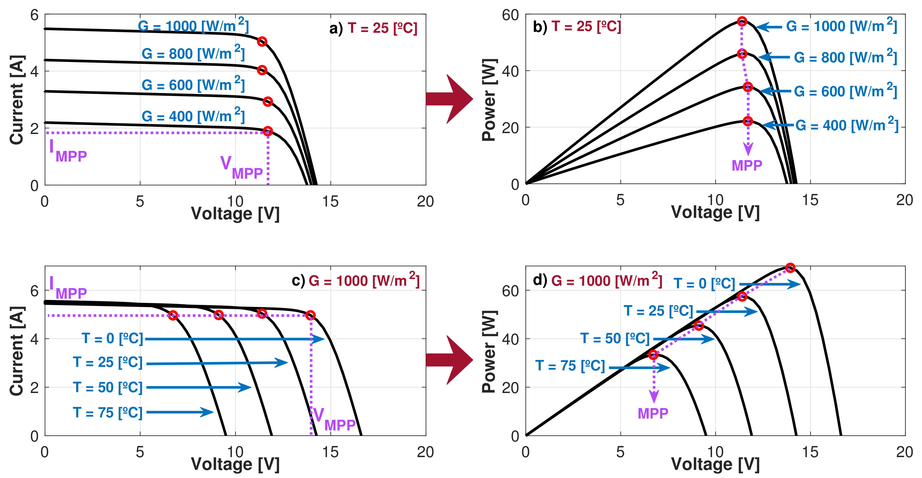
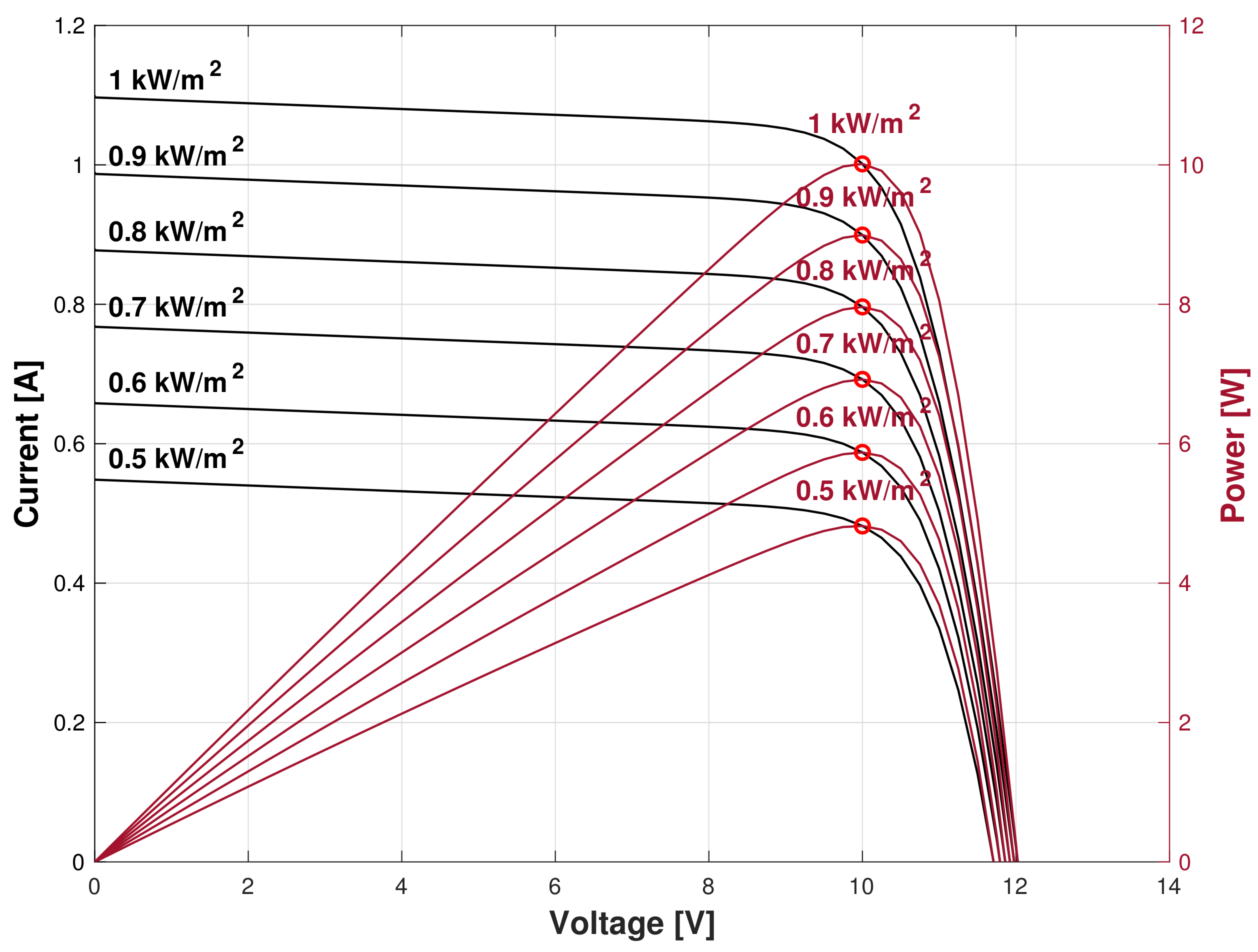
. Nevertheless, it is important to address the dynamic behavior of the PV array, which can be better analyzed through characterization of the power and current against voltage profiles, which were estimated through the mathematical model from Section 2 and are presented in Figure 14.
Additionally from Figure 14, it is worth highlighting that currents vs. voltage profiles were plotted against the left-hand vertical axis; meanwhile the right-hand axis presents the power vs. voltage features of the modules. On the other hand, the maximum power points (MPPs) are highlighted with red circles on each plot to address how the MPPs move under different solar irradiation conditions. Then, the profiles from Figure 14 also allow validation of the suitability of the designed PV array for the proposed case study, which would allow the DC–DC converter to operate at a maximum of 10 W under STC conditions.
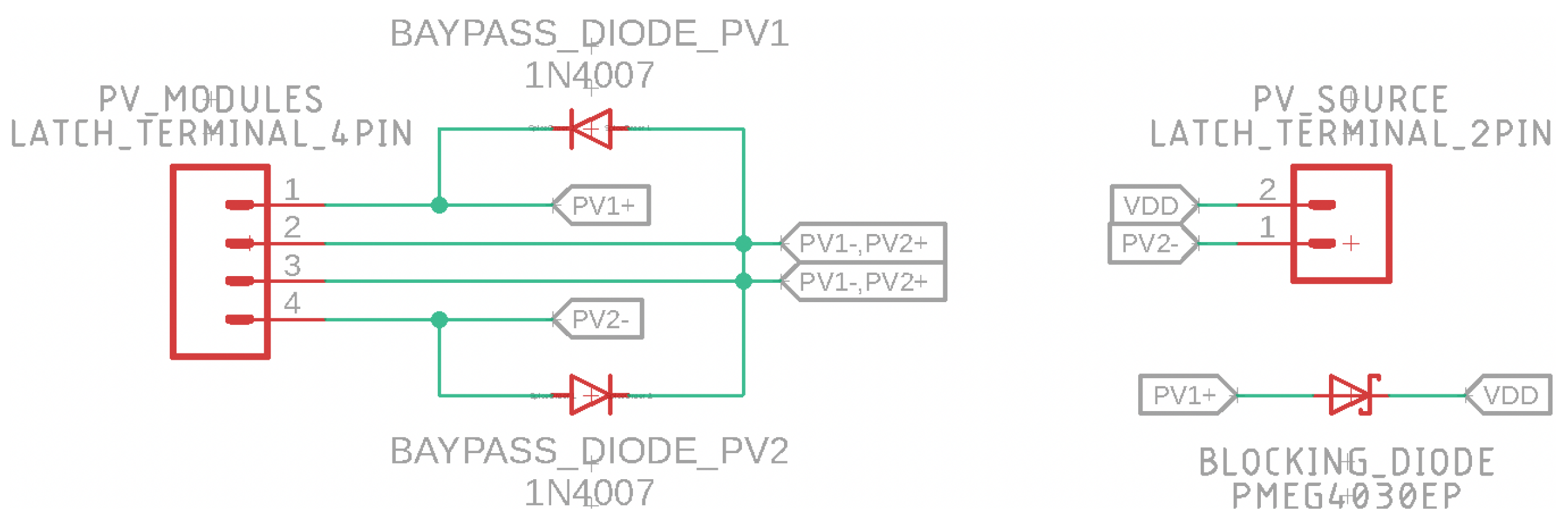
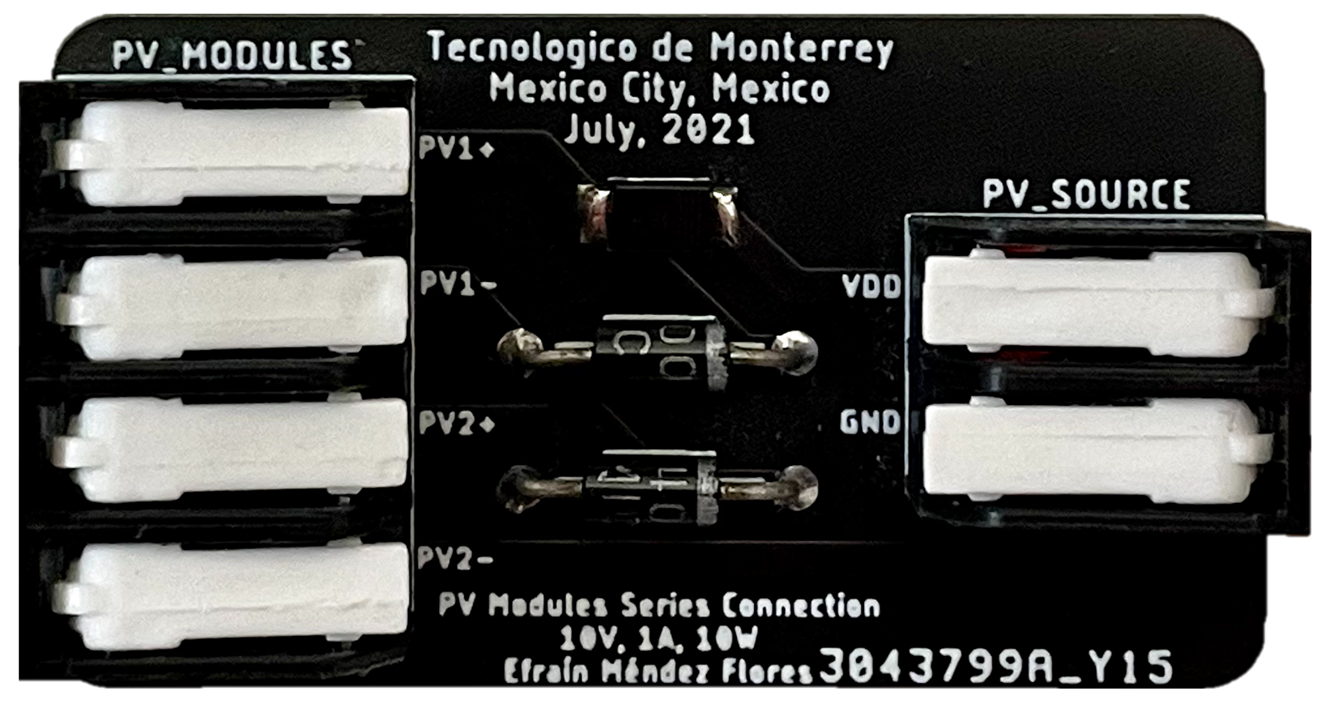
Moreover, to ensure reliable and safe connections between the photovoltaic modules and the DC–DC converter, a PCB was designed to avoid the risk of any connection errors throughout the experimental trials. Consequently, Figure 15 shows the schematics diagram of the designed circuit, where it can be also seen how both of the PV modules are internally connected in series to provide a single PV source for the DC–DC converter.
Additionally, Figure 15 shows where bypass diodes were added to the circuit, since those are a standard addition to prevent hot-spot phenomena, which, as explained by Solar Edge in [37], can produce serious damage to solar cells in the array, even causing them to ignite, particularly when sunlight does not uniformly hit the surface of the PV cells in the array.
Nevertheless, it is still important to highlight that the bypass diodes ideally do not provide any efficiency liability to the system, since they are acting as additional protection to the circuit and do not act when the PV array is operating in normal irradiation conditions—in other words, under conditions where both solar panels receive the same amount of solar energy on their surface. On the other hand, it is also clear in Figure 15 that we selected a Schottky diode as the blocking diode, since the blocking diode is continuously in contact with the output power supplied by the array and its only objective is to block reverse energy flow from the converter into the PV array. Thereby, 
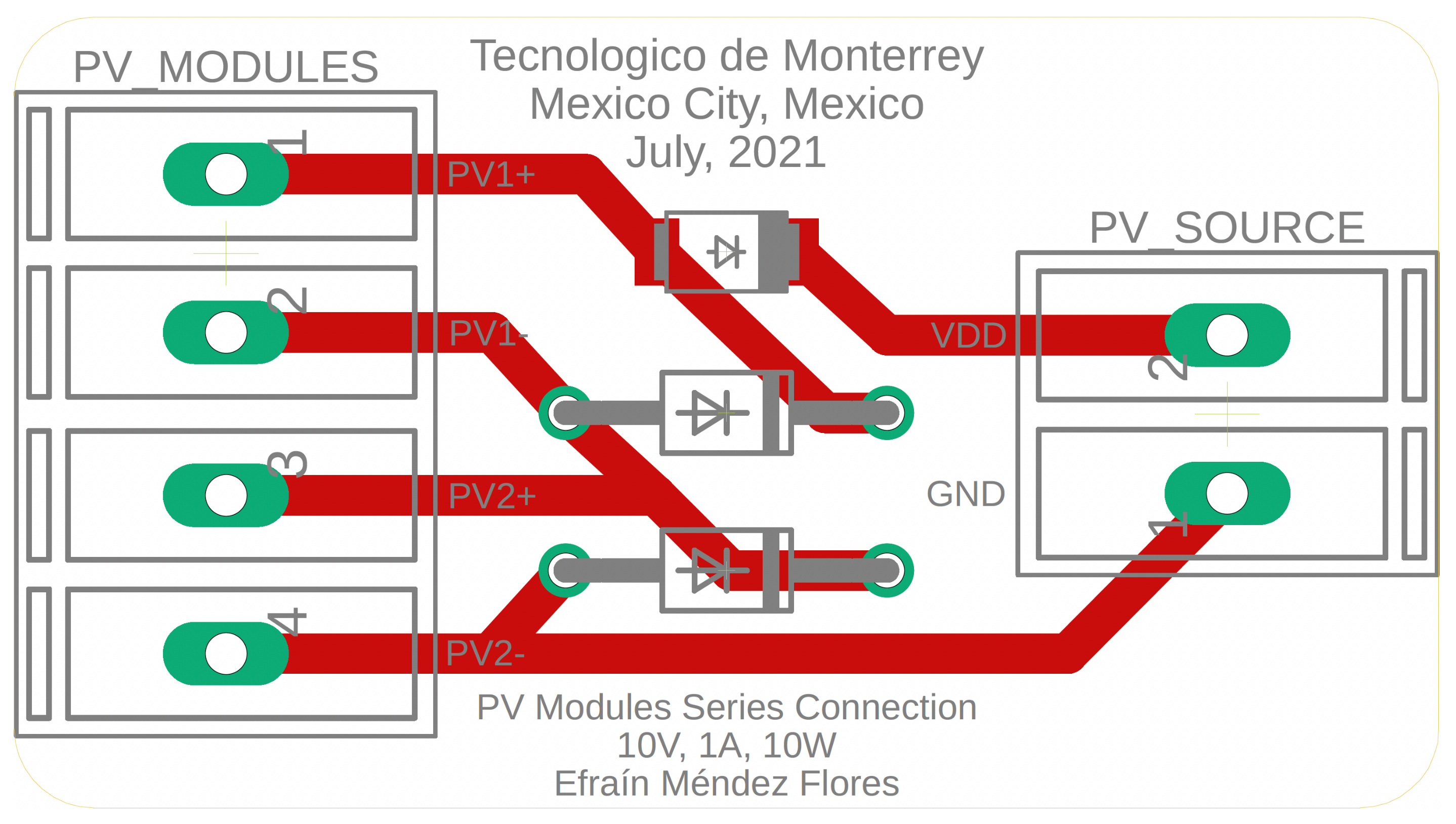
Figure 16 presents the PCB layout designed from the schematics from Figure 15.
In order to address the transition from circuit conceptualization to the manufacturing stage, the PCB design from Figure 16 was developed into an experimental PCB for the portable testbed; Figure 17 shows the printed board circuit with all the soldered elements, for which it can be analyzed that the PCB was designed as intuitively as possible, with multiple labels to ensure proper connections.
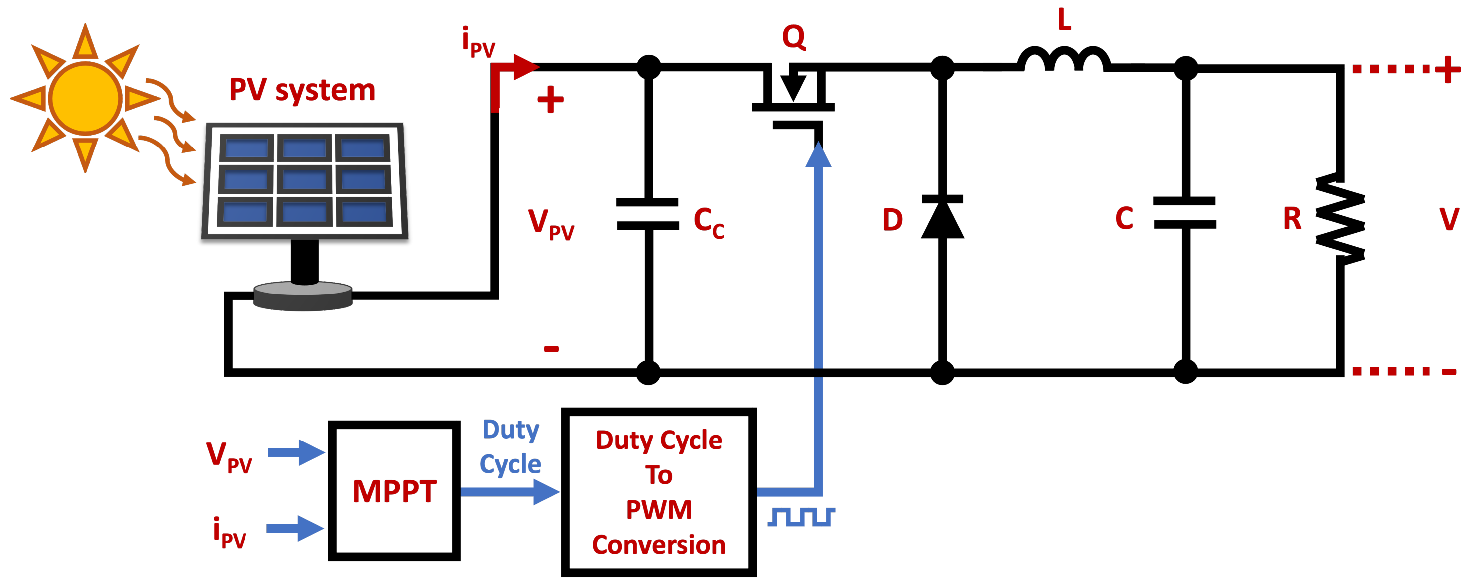
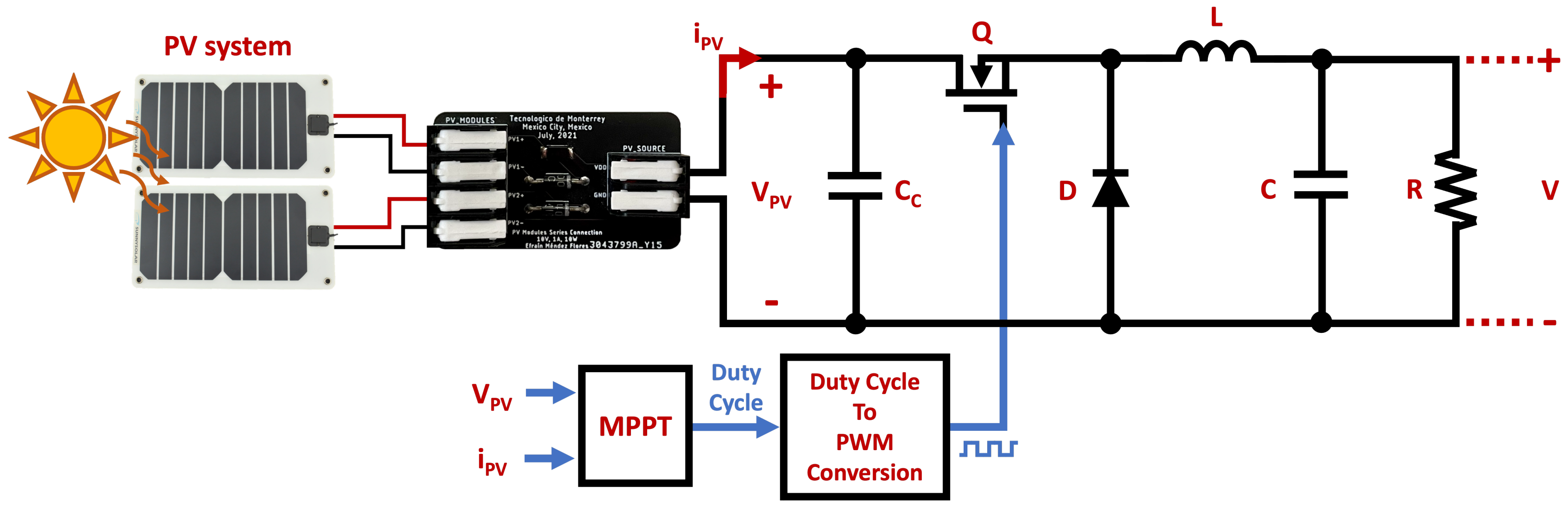
Then, to explain how the designed circuit together with the PV system are connected as the source of the DC–DC converter, Figure 18 embeds the connections of the PV cells and the manufactured PCB from Figure 17 into the case study topology from Figure 13, addressing where and how the elements are interconnected on the experimental testbed.
Nevertheless, since proper validation requires fully repeatable experiments to enable other researchers to achieve and reproduce the same results, the photovoltaic system was characterized to replicate its behavior by means of the Photovoltaic Array Simulator N8937APV, which, according to Keysight’s datasheet in [38], is a DC power supply with PV mode with an operating voltage range between 0 and 1500 V at a current between 0 and 30 A, which enhances dynamic simulations of the output characteristics of PV arrays under different environmental conditions such as temperature, irradiance, age, and even cell technology. Therefore, Keysight addressed in [38] that the equipment is particularly useful to enable quick and comprehensive tests for MPPT algorithms.
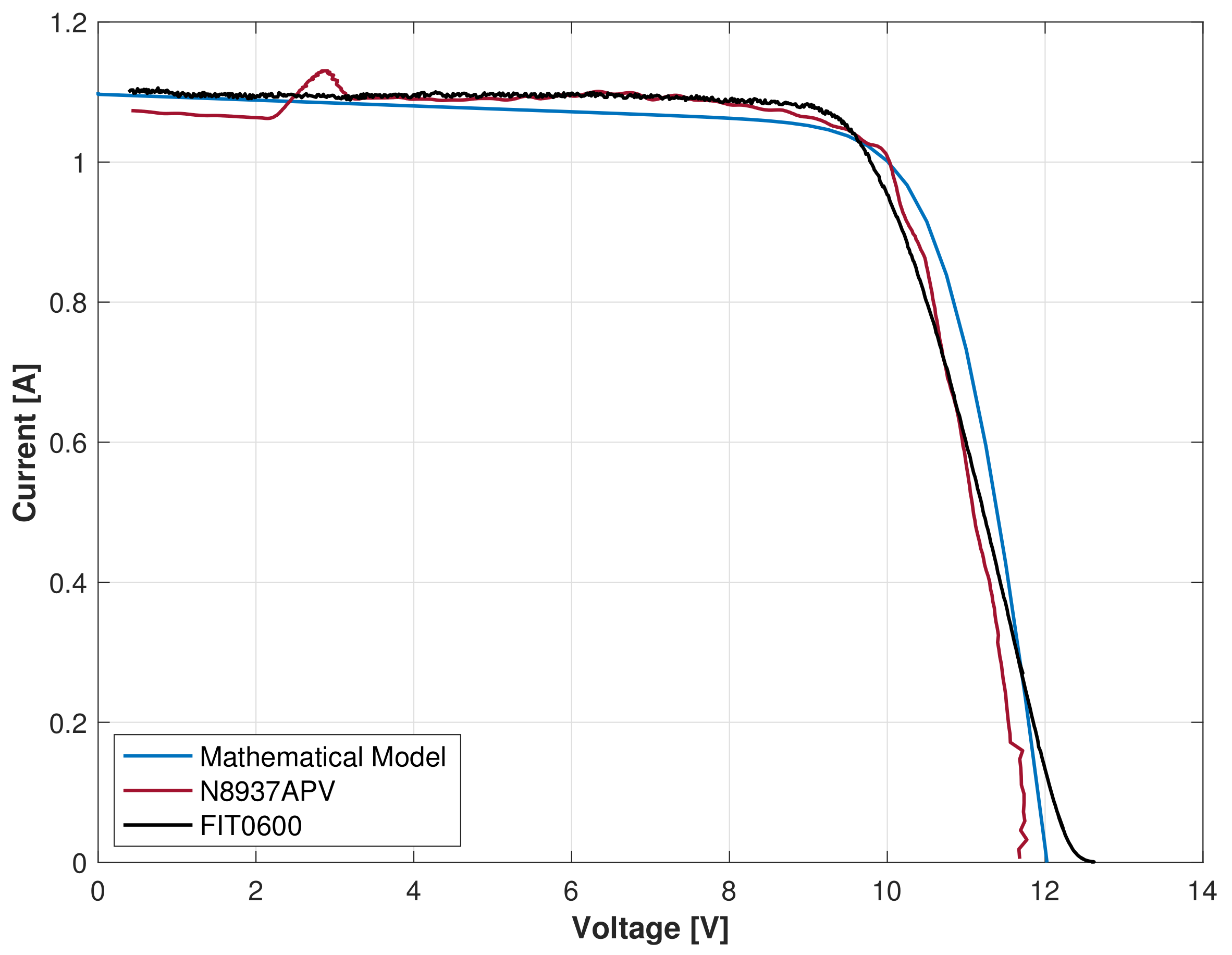
Then, to ensure proper representation of the dynamic features of the experimental PV array by its mathematical model, and also to enhance PV emulation through the N8937APV PV array simulator, the PV array and the N8937APV were subjected to variable voltage ramp characterization through a Keithley 2461 SourceMeter®, which, according to Keithley (Tektronix company) from [39], is optimized for characterizing and testing high-power materials, devices, and modules; the 2461 SourceMeter® features a 10 A/1000 W pulse current and 7 A/100 W DC current capacity. Consequently, the performed tests enabled us to obtain and compare the IV profiles of the PV arrays and the N8937APV, which, in addition to the mathematical model profile, are presented in Figure 19.
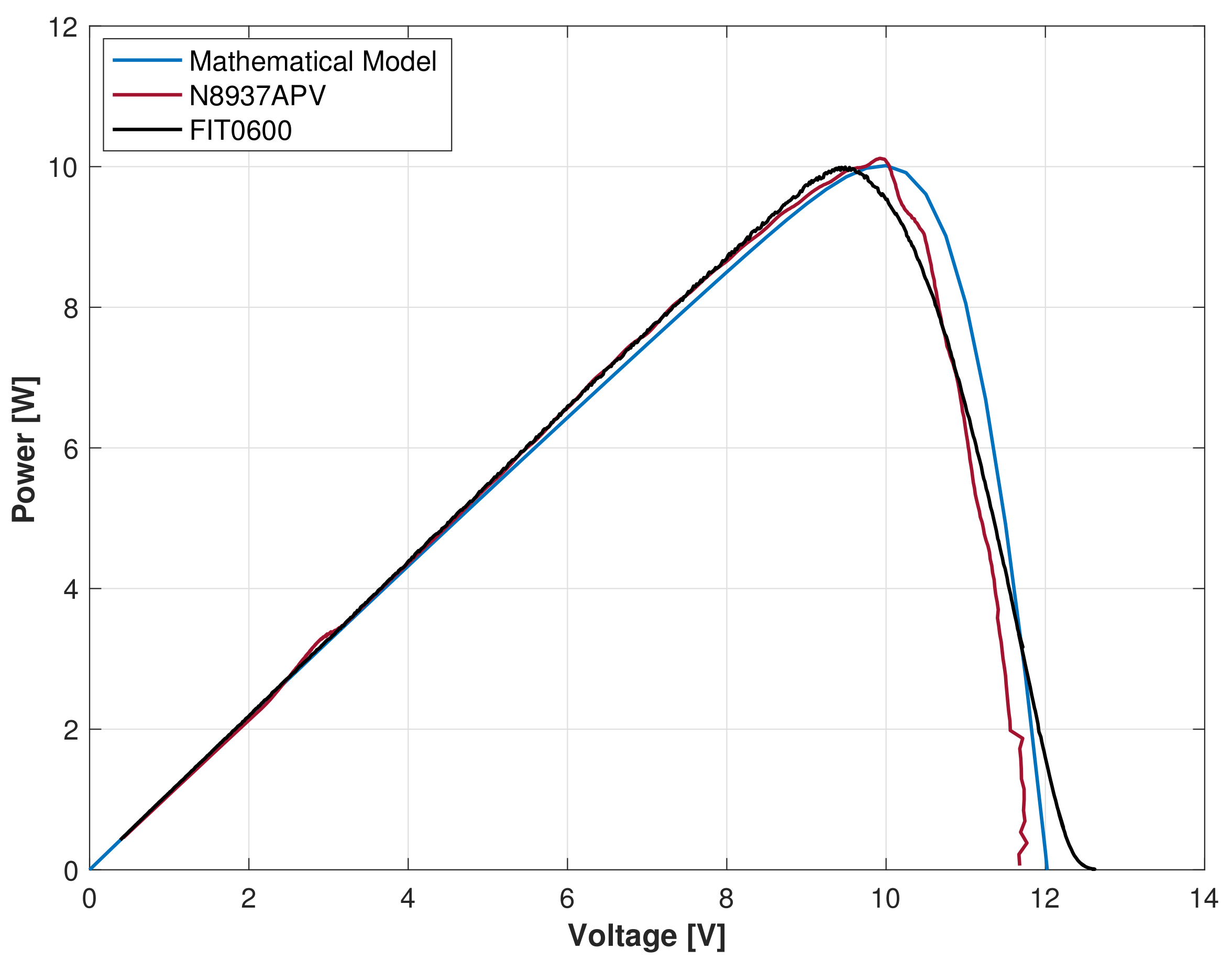
Consequently, we clearly validated that the IV dynamics of the mathematical model and the N8937APV are reliable representations of the dynamic features of the real FIT0600 PV array. Still, to fully address the power signal dynamic features, Figure 20 compares the power vs. voltage curves obtained through the acquired data from Figure 19. Moreover, Figure 20 allows graphical validation of the representation of the real PV array, mostly since the slopes are dynamically consistent between them, and the achievable MPP still remains around 10 W.
Furthermore, in order to sustain that the dynamics of the N8937APV and the mathematical model are valid representations of the real power behavior of the PV array, the errors and the precision of the representations against the experimental PV arrays were estimated through the quantified data; the N8937APV PV array simulator achieved 12.8089% average error that led to 87.1911% precision; meanwhile, the mathematical model compared to the experimental array achieved 84.7796% precision with an average error of 15.2204%.
Thereby, to enhance the reproducibility of the results and to ensure equal test conditions in all the experimental validation test trials, the structure presented in Figure 18 was rearranged into the experimental topology addressed by Figure 21, which can be inferred as valid through the dynamic comparison from Figure 20.
Therefore, the following section details the main features of the designed DC–DC buck converter for the case study that enabled the experimental validation trials for the proposed improved EA-based MPPT algorithm.

6.2. DC–DC Converter

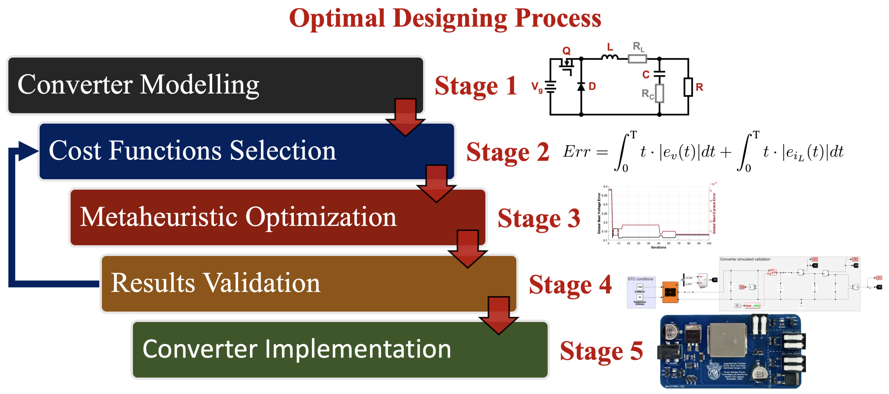
After exploring the main features of the PV source designed for experimental validation, the DC–DC converter developed for this application was developed through the optimal design methodology addressed in 
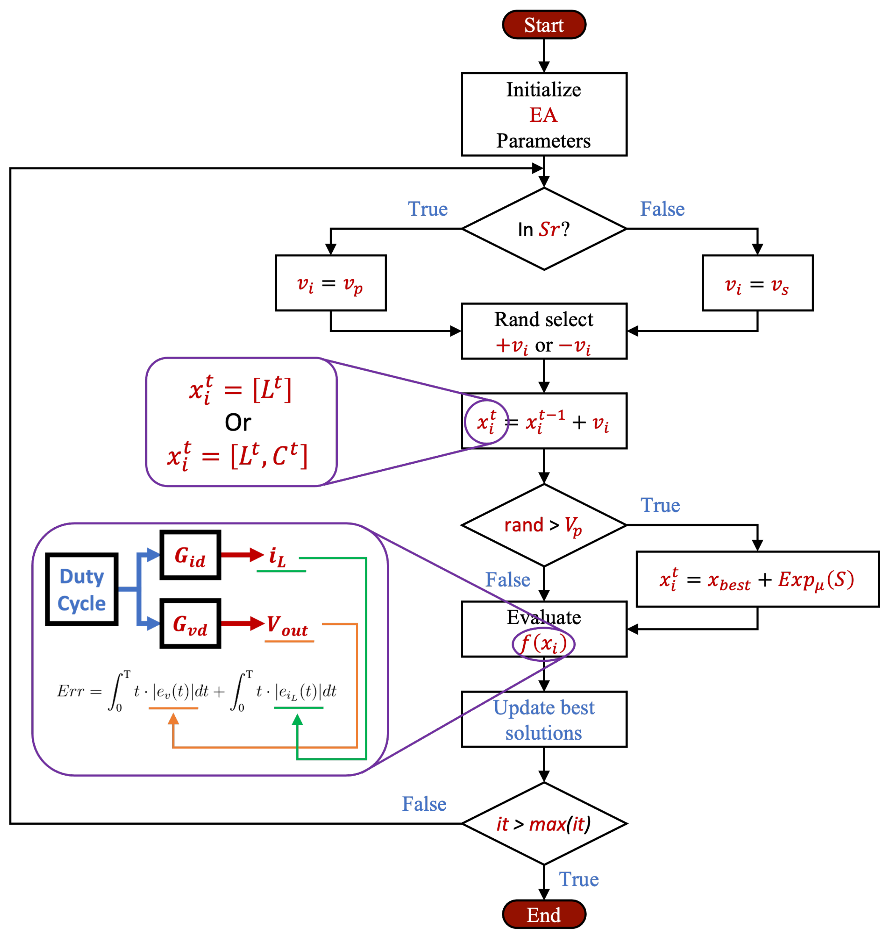
Section 5. Then, the classic EA was implemented for the design technique, where the optimization was carried out through a set of 20 epicenters (searching agents) through 100 iterations in each optimization trial (three trials), where the results were taken from the mean values among the trials; additionally, the algorithm was configured to find an inductance with low ESR, which, together with the new capacitance, could enable fast dynamic behavior while retaining low ripple-effect on the converter, which obeys the requirements of the continually induced perturbations from the MPPT algorithm.
Therefore, 
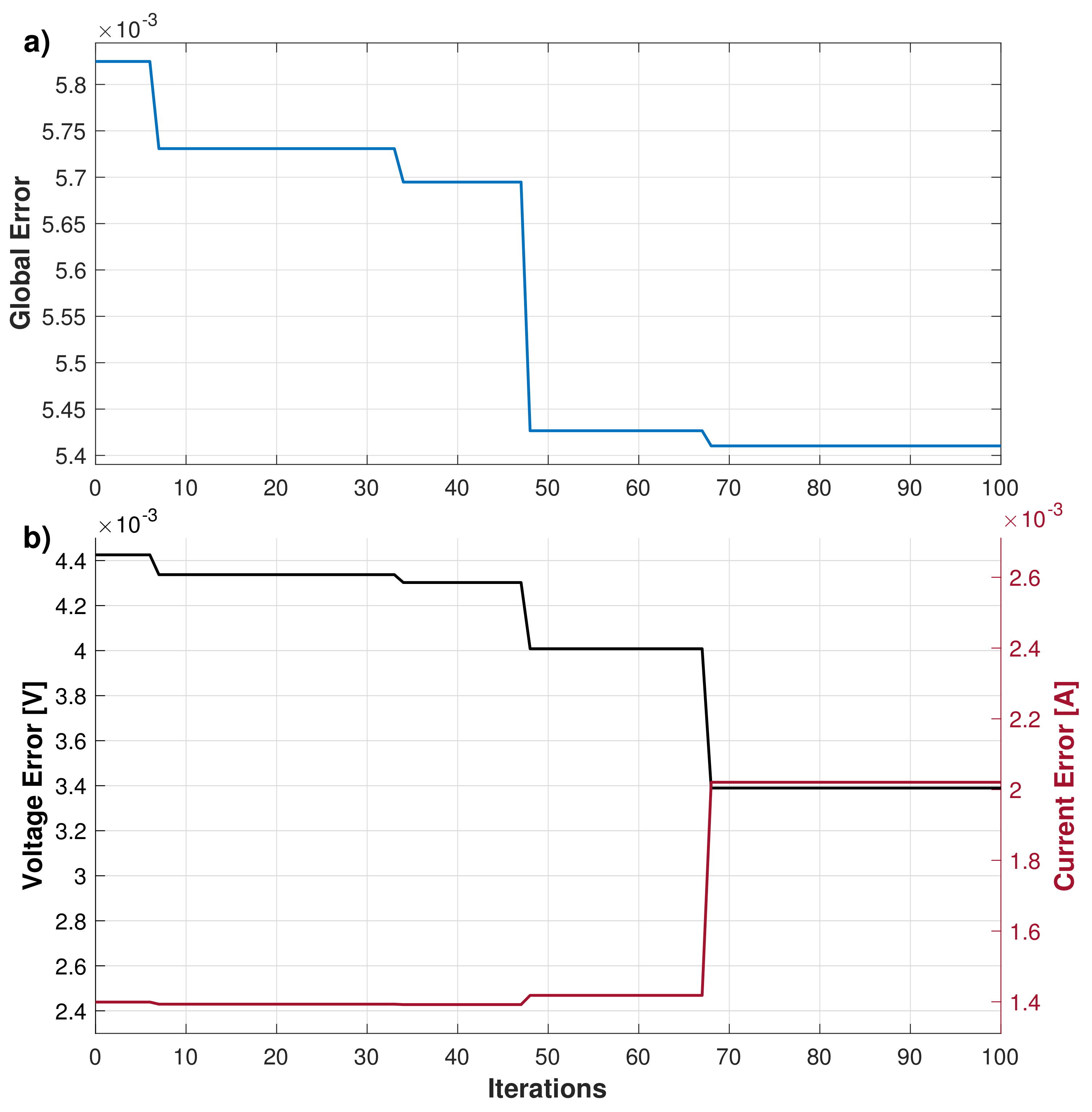
Figure 22 presents the convergence plots of the optimization process throughout the 100 iterations. On the one hand, Figure 22a shows how the global error, estimated through Equation (10), is reduced through iterations. On the other hand, Figure 22b breaks down the global error profile into its voltage and current components, since Equation (10) highlighted, through e v and e i , where the ITAE from the voltage and current errors are estimated.
Consequently, profiles from Figure 22a,b show how multiobjective optimization enables equilibrium between the errors, where the metaheuristic algorithm finds the optimal components for which the converter has the best performance for the given application (MPPT tests in this case). Accordingly, the inductance and capacitance results optimized by the algorithm meanly settled at 79.677 μ H and 215.64 μ F, with a mean global error measured through Equation (10) of 0.0054103 after 100 iterations (as seen in Figure 22a).
Subsequently, the experimental capacitor and inductor were selected through study of the nearest available commercial values; thus, the selected capacitance was an aluminum organic polymer 220 μ F capacitor. Meanwhile, to meet the dynamics and efficiency requirements of the application, the inductance was taken as a fixed-shielded high-current molded 82 μ H power inductor. Then, the main parameters from the selected inductor are presented in Table 3, Table 4 presents the main parameters of the selected capacitor for the circuit, and 
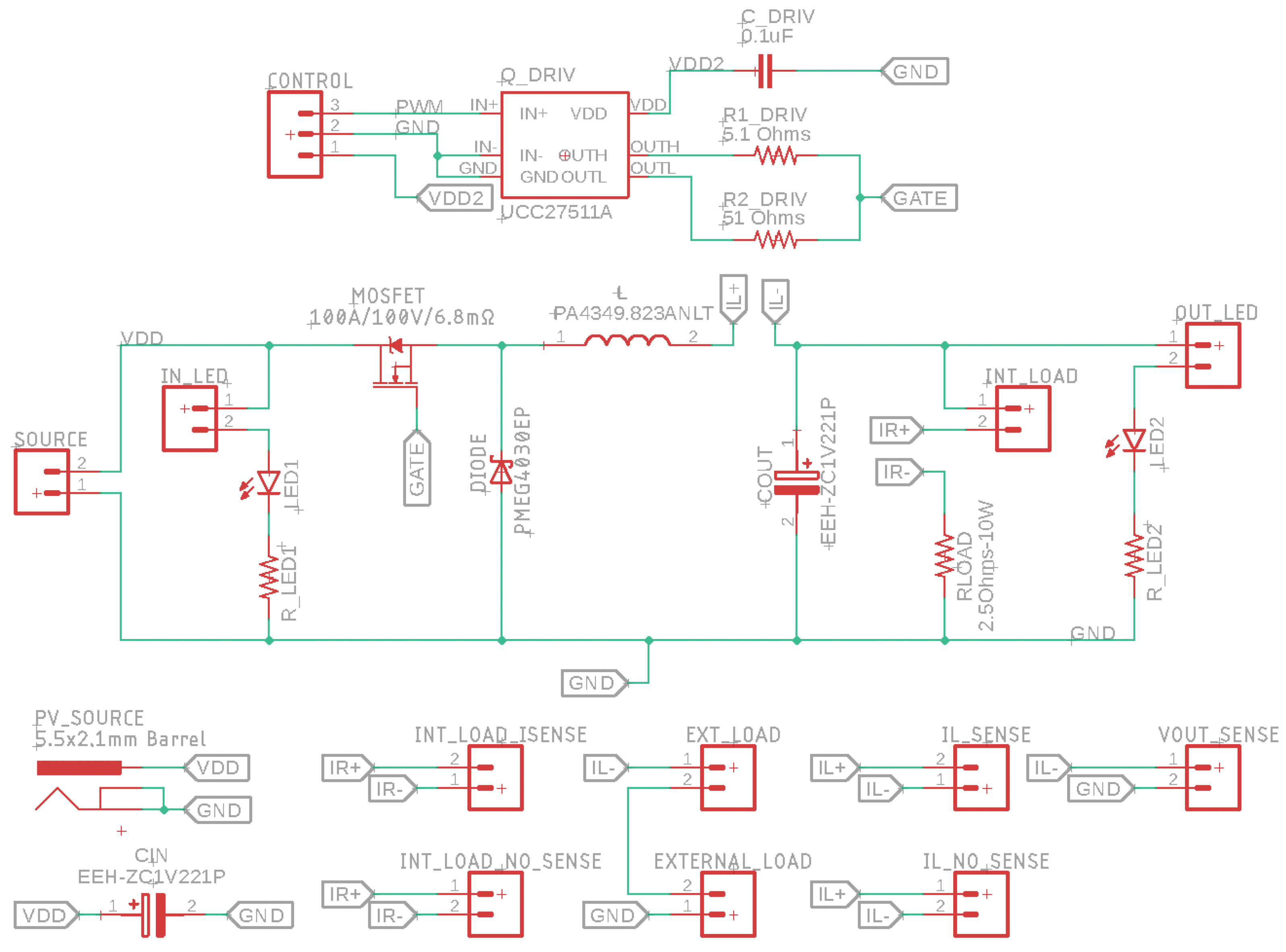
Figure 23 shows the schematics diagram of the circuit and where the capacitance and the inductance were implemented.
Additionally, Figure 23, shows at the top the required connections for the MOSFET’s gate driver, which was selected to be the single-channel gate driver UCC27511A, as also addressed in the experimental implementation presented by Mendez-Flores, E., et al. in [29]; since according to the datasheet presented by Texas instruments in [42], it is a compact, high-speed solution suitable for DC–DC converters and also provides parasitic Miller turn-on effect rejection.
Moreover, in the middle of Figure 23, the main structure of the designed DC–DC converter is presented; the figure also presents how the input and output LED indicators can be decoupled from the system in order to enhance the possibility of tests through the minimal required components without the case apart when fast input/output verification is required.
Additionally, two different PV source connections were added to the design; on the one hand, 5.5 × 2.1 mm barrel was provided as an additional safety measure, which allows the user to avoid the possible scenario where the PV source is mistakenly connected with reversed polarity. On the other hand, source header pins were also provided on the design to enable tests with additional fixed sources, thus, both headers enable a suitable option for a different external sources for the system. The CIN capacitor below the barrel jack is the coupling capacitor previously described in Figure 18, the capacitance of which is the same as the output capacitance described in Table 4.
Hence, from the bottom of Figure 23, the two-pin connectors provide reconfiguration options for the converter; if both INT_LOAD_NO_SENSE connectors are joined, the INT_LOAD_SENSE terminals are useless since those terminals are bridged, but if they are not bridged, INT_LOAD_SENSE can be used to connect a current sensor to monitor the current through the internal load of the circuit. Still, the internal load (2.5 Ω ) can be removed from the test trials if the INT_LOAD terminals are detached.
Similarly, if the EXT_LOAD headers are bridged and the INT_LOAD terminals are separated, an external load can be attached to the converter to enable tests under different load experiments; therefore, the external can be connected and monitored through the EXTERNAL_LOAD terminals. Finally, when the IL_NO_SENSE terminals are not united, the current through the inductance can be monitored through an external sensor at the IL_SENSE terminals.
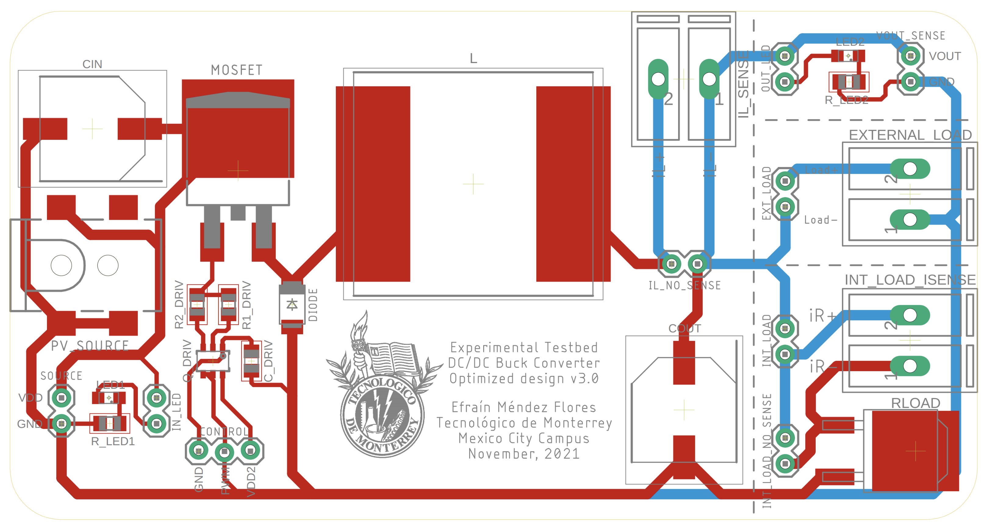
Thereby, under those circumstances and with those design considerations in mind, Figure 24 presents the PCB layout designed for the DC–DC converter implementation for the PV experimental case study, where all the elements from 
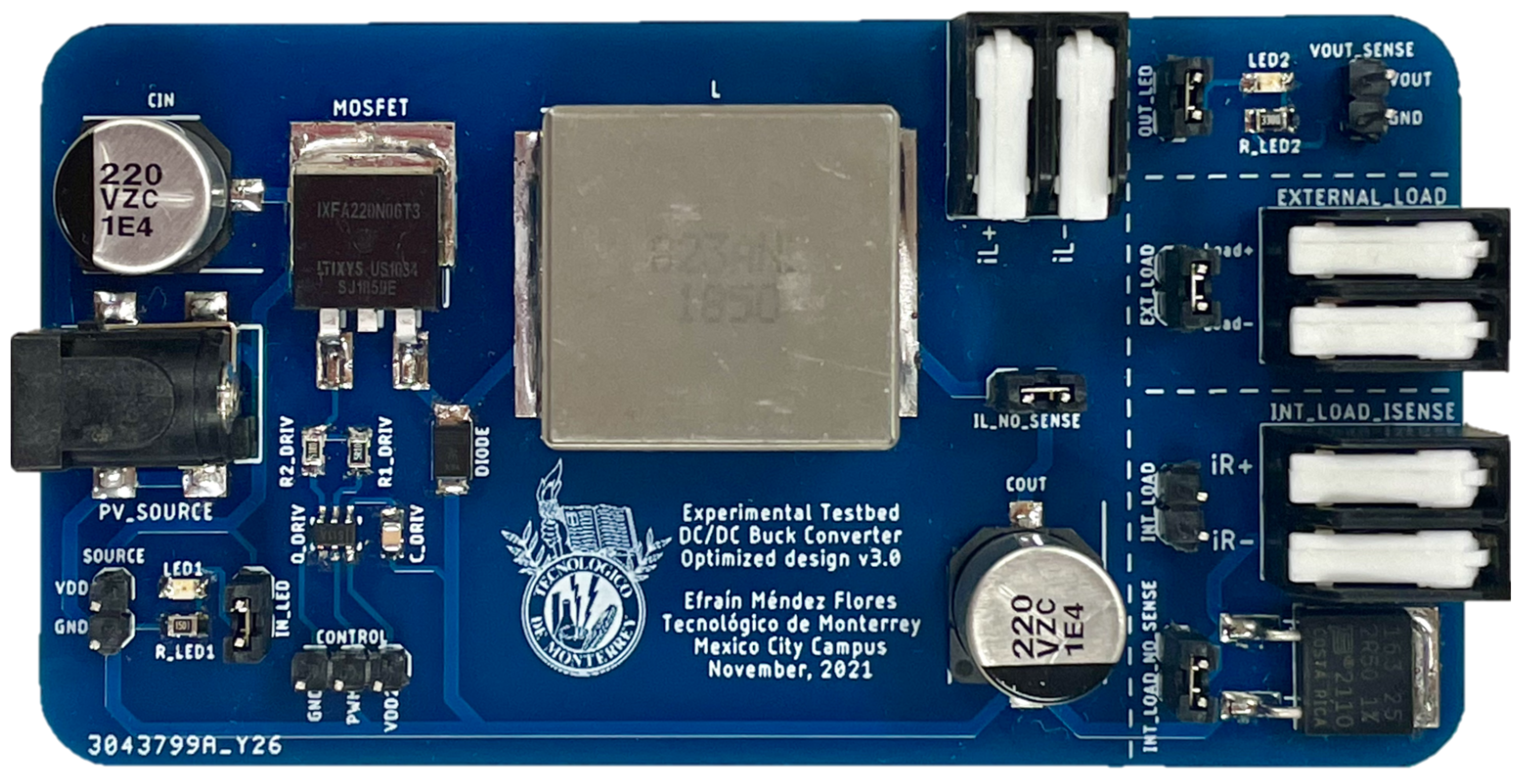
Figure 23 were arranged and routed for the manufacturing stage of the converter. Then, Figure 25 presents the manufactured PCB of the DC–DC converter.
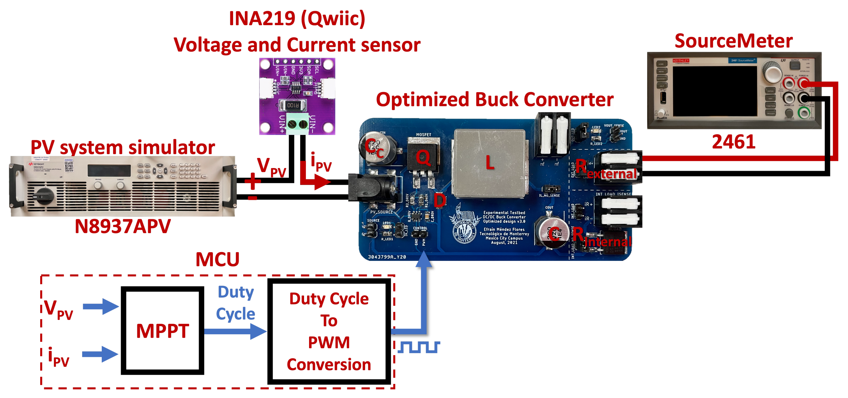
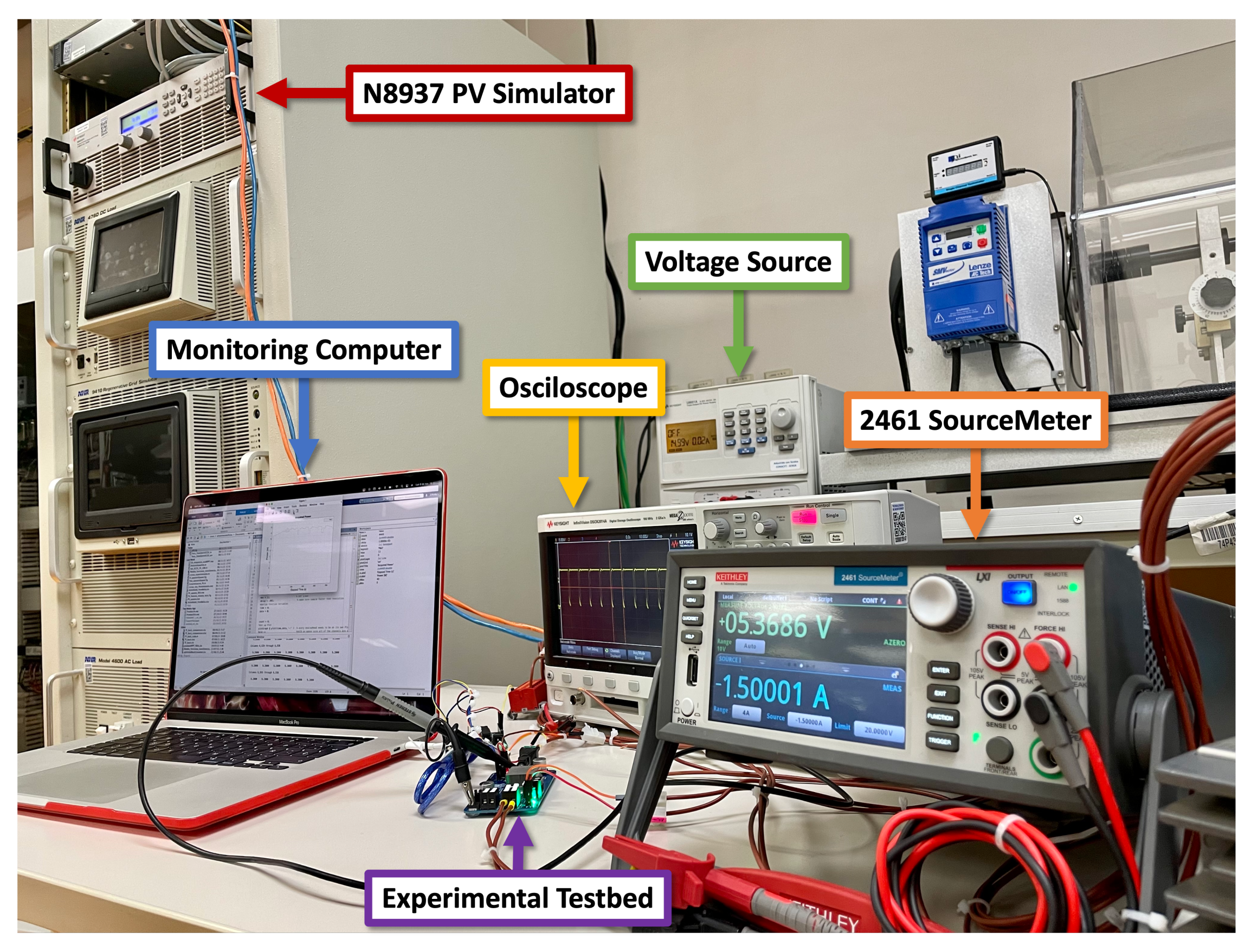
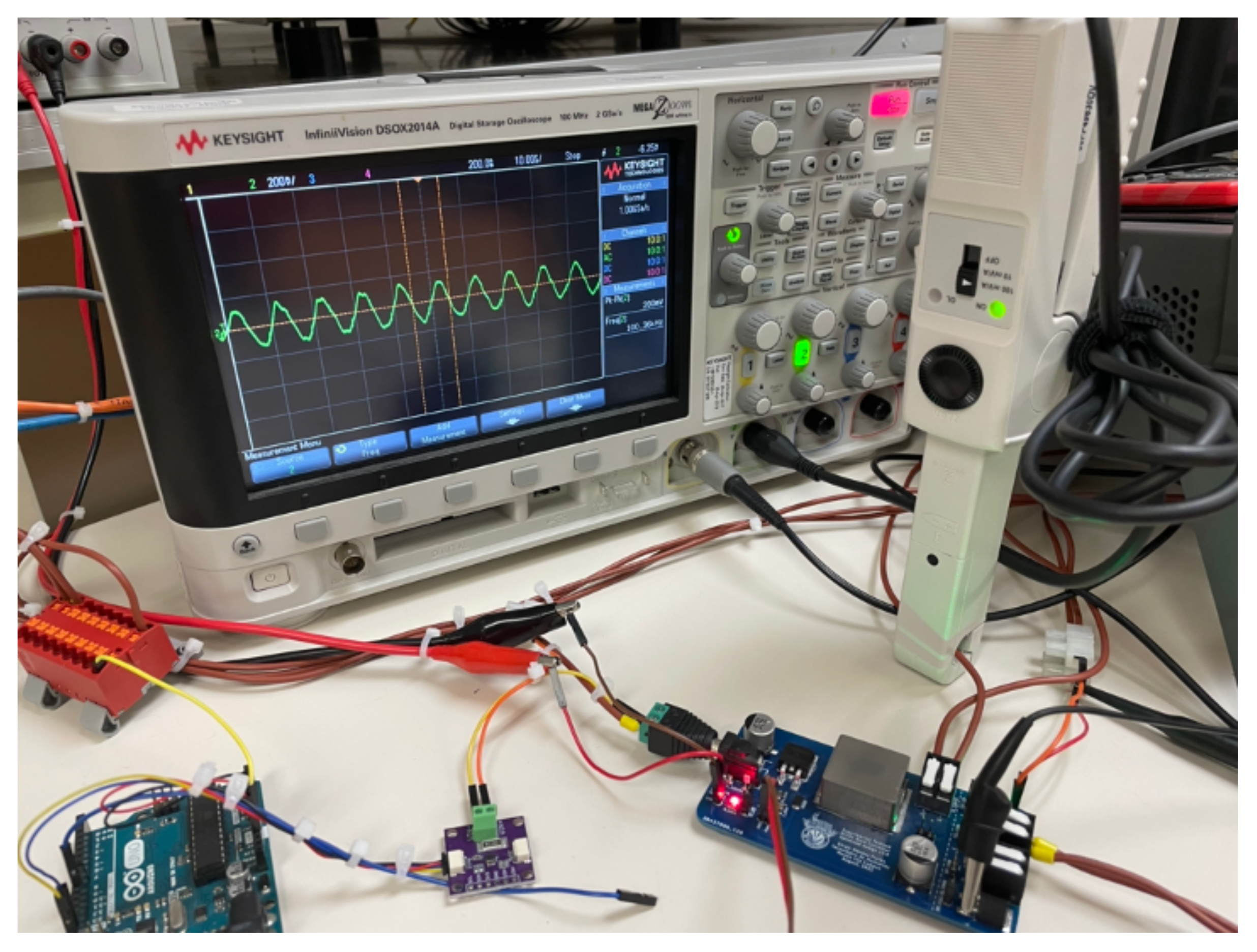
Hence, keeping up with the figure sequence that shows how the experimental frame was built for the validations tests, 
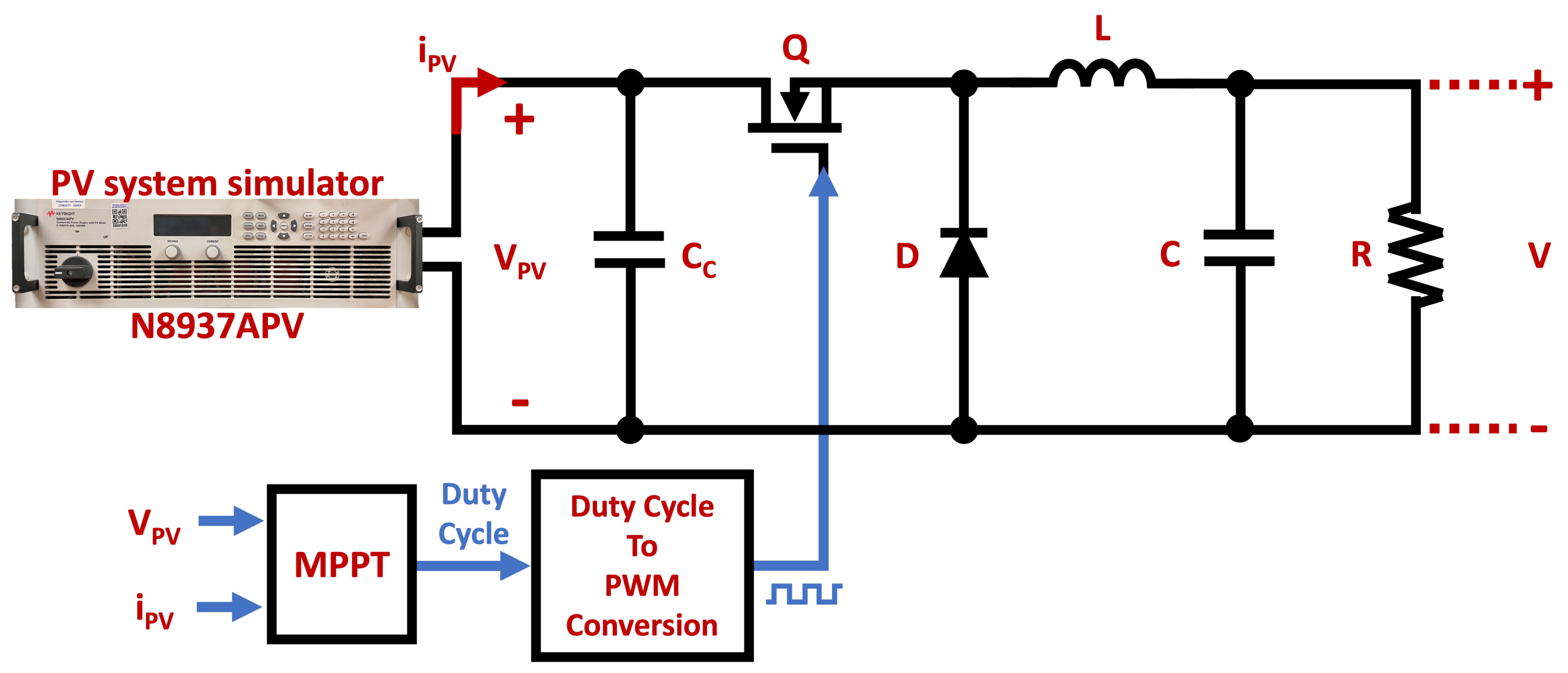
Figure 26 presents the case study topology, where integration of the N8937APV PV array simulator, the 2461 SourceMeter®, and the optimized buck converter (from Figure 25) is presented. Additionally, from Figure 26, it can be seen where the main elements and variables from Figure 13 are implemented; also Figure 26 highlights the MPPT and the PWM stages, addressing where the microcontroller unit (MCU) acquires and processes the data to provide the control signal to the system.
Yet it is critical to mention that from now on, the data acquisition process regarding the voltage, current, and power signals for the implementation and evaluation of the proposed MPPT algorithm are carried out through the INA219 (Qwiic) module, which is based on the INA219 power monitor with I 2 C interface presented by Texas Instruments in [43]. Then, Qwiic is a rapid prototyping standard developed by Sparkfun® that uses 4-pin JST connectors to quickly interface development boards with sensors, microcontrollers, and displays, among others things.
The INA219 (Qwiic) module was selected for the experimental tests since the module provides a reliable solution that reports current, voltage, and power through I 2 C protocol with up to 1% precision, suitable for tracking solar power generation applications. According to [43] by Texas Instruments, the sensor can measure voltage up to 26 V and current up to 3.2 A, which fits on the 10 W case study proposed to work at 10 V and 1 A at the PV terminals.
Consequently, 
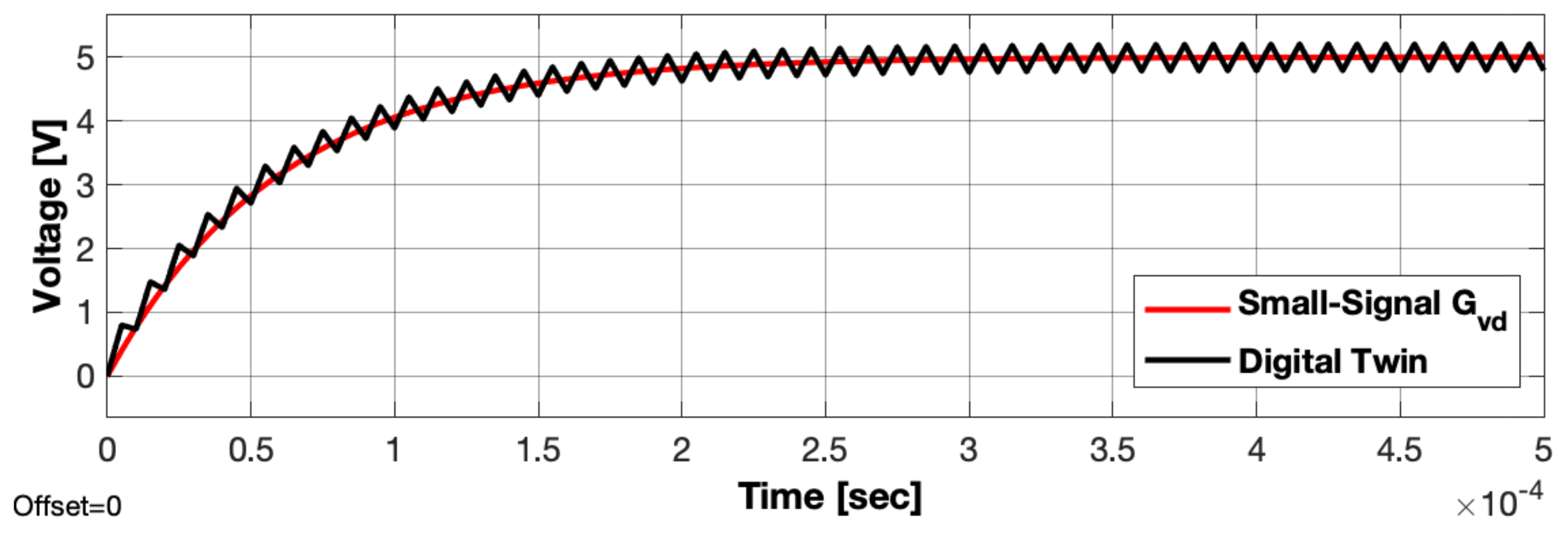
Table 5 summarizes the parameters of the buck converter for which its design was optimized for the PV case study. Nevertheless, since the novel optimal design methodology validated by Mendez-Flores, E., et al. in [
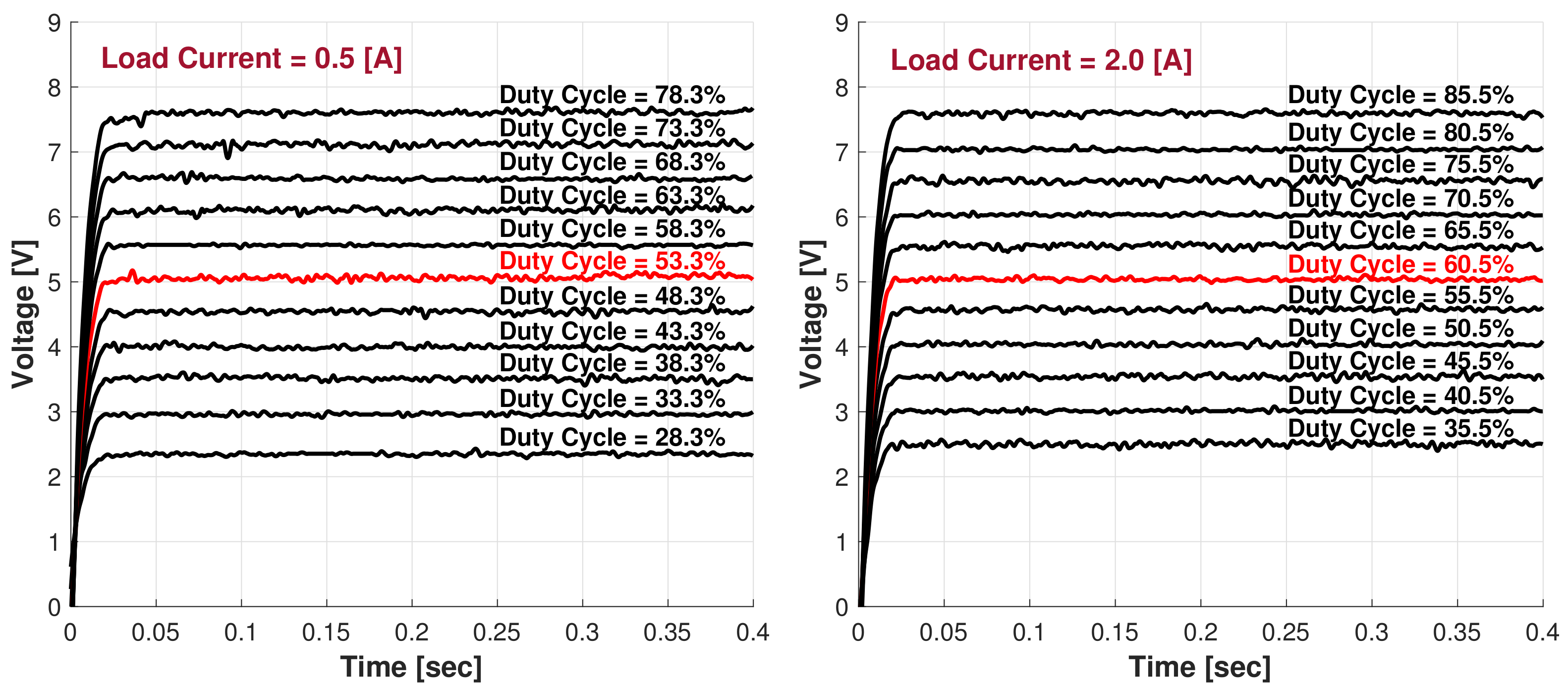
29] is acknowledged as one of the main contributions of this work, the dynamic performance profiles of the experimental converter through multiple duty-cycle step signals are provided in the following section of this work as part of the featured results.
Therefore, the following section presents the main results of the experimental integration case study proposed to validate how the contributions of this work enhance smarter photovoltaic systems. Then, among the results from the following section, it is seen how the dynamic features of the optimized converter enable a prominent testbed for the algorithm’s validation.

7. Results

Seeking to validate the contributions of this work, the developed results in this research are mostly divided into two main subsections: the first one presents the main experimental results of the DC–DC converter optimally designed for the PV case study; meanwhile, the second one discusses the results from the perspective of the EA-based improved MPPT algorithm embedded through the converter.
Thereby, Figure 27 presents the implementation of the testbed integrated with the case study topology and interconnected to the laboratory’s equipment just as schematized in Figure 26, with the N8937APV PV simulator and the 2461 SourceMeter® are also shown. Then, the following subsection addresses with greater detail the efficiency and dynamics evaluation of the converter through the addressed equipment.

7.1. Optimized Converter Experimental Results

Since for this case study the DC–DC converter was designed to provide a nominal 5 V of output voltage at 2 A of output current at the MPP, the experimental testbed was subjected to a current sweep to evaluate the efficiency of the design under different current loads, which allowed validating the suitability of the converter for the 10 W proposed PV application.
Therefore, Figure 28 presents the efficiency profile of the converter over the operating range of the PV system. Hence, it is proven that the optimal design is perfectly suitable for the case study, since the buck converter achieved almost 90% efficiency at the nominal output power for the converter, which would efficiently harness energy at STC of the PV array when it is supplying the maximum achievable power.
Moreover, Nowakowski, R., and Tang, N., in [44] explain that commercial nonsynchronous buck converters meeting the same power range of operation can usually achieve up to 85% efficiency, which ensures that the converter designed for experimental validation has outstanding features, even compared to some commercial converters. Then, after validating that almost 90% efficiency is achieved under the STC conditions of the proposed PV case study, the dynamics of the buck converter had to be evaluated in order to feature a proper implementation of the MPPT.
Thereafter, Figure 29 shows the dynamic behavior of the converter against different duty cycle (control signal) steps, which validates that under the required conditions, the control signal is still achievable even under the greatest current loads that the PV array can provide. Yet it is important to address that the data acquisition for the voltage profiles from Figure 29 was acquired through the Keysight InfiniiVision DSOX2014A Digital storage oscilloscope, which has a bandwidth of 100 MHz and a maximum sample rate of 2 GSa/s, which is more than enough to uncover the dynamic performance of the circuit.
It is important to address that the voltage profiles from Figure 29 were obtained by determining the duty cycle needed to meet the nominal conditions of the converter under different continuous current loads, which were taken from the current boundaries in the proposed 10 W case study. Additionally, to feature the precision that the control signal can achieve, a duty-cycle sweep was performed around the nominal duty cycle for which the converter finds the 5 V output voltage.
Hence, it is clear from Figure 29 that the converter achieves remarkable precision through duty-cycle changes, since the step changes allow us to obtain fine results at the output voltage of the converter, which is a feature that was also a key result from the first experimental validation of the design methodology provided by Mendez-Flores, E., et al. in [29]. Therefore, the consistency of the dynamic features of the converters designed through the contributed methodology double-checks the reliability and suitability of the design methodology for multiple applications.
However, Figure 29 also allows evaluation of the transitory state of the system through the slope of the voltage profiles, which provides enough information to analyze the suitability of the converter for MPPT applications, since it was validated in [21] by Mendez-Flores, E., et al. that a typical sample rate for MPPT algorithms can be similar to or near 0.1 s.
Nevertheless, it is still relevant to evaluate the inductance current of the optimized design in order to fully validate whether the design objectives were completely fulfilled, which is why Figure 30 shows how a hall-effect current tip was connected to the IL terminals of the converter, which allowed us to acquire the inductance current signal of the converter operating at an output current of 2 A.
Therefore, Figure 31 shows a screenshot from the oscilloscope taken during the inductance current evaluation, which validates once again that the proposed design methodology leads to converters with reduced ripple effect. Still, Erickson, R. W., and Maksimovic, D., in [31] explain that for buck converters, the ripple can be defined as presented by Equation (13).
Δ i L = V g V 2 L D T s
where Δ i L is the ripple current through the inductor, which is defined as the average-to-peak current. Then, the theoretical ripple of the converter should be near 0.1524 A, which represents almost 7.6% of current ripple. Subsequently, Erickson, R. W., and Maksimovic, D., in [31] explain that commercial converters typically achieve Δ i L values that lie in the range of 10% to 20%, which sustains even more the quality of the designed converter, since Figure 31 measured a 0.140 A Δ i L .
Still, to properly evaluate the experimental data regarding the ripple on the inductance current, the acquired data were post-processed to digitally obtain and evaluate the experimental Δ i L results. Thus, Figure 32 presents the current ripple data acquired from the oscilloscope, but this time, they are plotted in the MATLAB environment and are additionally compared to the simulated i L profile of the converter.
Then, the experimental inductance current ripple Δ i L was estimated through the data plotted in Figure 32, leading to the precise 0.1468 A calculated ripple, which is transduced into almost 7.3% of current ripple. Therefore, the simulated behavior of the converter was 96.32% precise when compared to the dynamics of the experimental converter. Henceforth, after validating that the dynamic features of the converter were suitable for the case study, the MPPT experimental results were carried out through the optimally designed converter and are presented in the following section.
Consequently, this subsection fully validated and experimentally double-checked the claimed contributions of the optimal design methodology proposed by Mendez-Flores, E., et al. in [29], where the quality of the provided design perfectly enhances the quality of the methodology.

7.2. Improved MPPT Experimental Results

After validating that the dynamics of the experimental DC–DC converter design were reliable for MPPT applications, we present the results from the experimental validation tests performed to ensure the suitability of the EA-based MPPT algorithm for real-life applications. Nonetheless, in the same validation track, an Arduino UNO development board was taken as the MCU to embed the algorithm, since it is a well-known testbed for rapid algorithm prototyping. Still, the Arduino UNO has limited processing capacity based on the ATmega328P microcontroller, which under the development board design can only achieve 16 MHz clock speed and has 32 KB of flash memory, 2 KB of SRAM, and 1 kB of EEPROM.
Nevertheless, the Arduino UNO enables validation of the simplicity of the contributed MPPT, with easy suitability for the application through the pre-existing INA219 current and voltage sensor libraries, which are sustained by the few required connections, as appreciated in Figure 32. Still, it is important to address that the updating time for all the algorithms tested in this paper was 50.008 mSec.
Hence, the results from the contributed EA-based MPPT algorithm are evaluated and compared against the classic P&O algorithm (as shown in Figure 33) in order to provide a simple benchmark to address the magnitude of the results through a state-of-the-art case, similar to the results validated in [21] by Mendez-Flores, E., et al., where the simulated features of the algorithm were peer-reviewed and published due its contribution to MPPT applications. Yet different from the validation presented by [21], this case study did not consider the PSO-based MPPT for the benchmark comparison due to the constant oscillations from the optimization process, which, in addition, to the parametric calibration features of the algorithm, may represent a risk for the whole system, mainly due to the aggressiveness of the tracking behavior, also explored by Dolara, A., et al. in [19].
As consequence, Figure 33 addresses the dynamic behavior of both EA-based and P&O MPPTs, showing the energy harvested through time for both algorithms. Thus, it can also be analyzed from Figure 33 that the EA-based MPPT managed to find the MPP faster compared to P&O, and both algorithms behaved similarly to the simulated results presented by Mendez-Flores, E., et al., in [21]. Therefore, the power profiles from Figure 33 allow evaluation of the consistency of the results, where the EA-based algorithm shows once again that its greatest contribution is found in its MPP tracking speed, which exploits more time for solar irradiation to be received on the photovoltaic system.
However, to provide a fair comparison between the algorithms, four more trials were performed in addition to the test trial from Figure 33 to address the heuristic features of the EA-MPPT. Yet since the sampled graphs would overlap between them, it would be difficult to simultaneously analyze and compare the dynamics of the experimental testbed under all the test trials. To overcome the issue and to have a better graphical evaluation, Figure 34 presents how the averaged smoothed profiles are obtained to still represent the dynamics of the converter. Hence, the same profiles from Figure 33 are presented to validate that the dynamic features of the curves are still conserved.
Then, after dynamic feature validation from Figure 34, Figure 35 shows the averaged experimental profiles of the P&O MPPT algorithm compared against five test runs of the EA-based algorithm (since P&O is not heuristic); it is clear that the EA-based MPPT improved the maximum power point tracking process even under its worst heuristic behavior, which allows us to verify the proposed EA-based MPPT as a reliable improvement for dynamic optimization.
Yet in order to quantify the results from the MPPT tests for each algorithm, Table 6 shows the quantified power data from each EA-MPPT test trial compared to the P&O algorithm, which, for instance, sustains that all the EA-based MPPT trials managed to harness more energy through time than the P&O algorithm, which was clear from the dynamics featured in Figure 35. It is important to mention that the red values from Table 6 highlight the best features in terms of the different evaluation features.
Moreover, Table 6 remarkably validates the consistency of the simulated features of the EA-based and P&O MPPT algorithms, as compared to the results addressed by Mendez-Flores, E., et al., in [21], since in all the tested cases, the EA-MPPT managed to achieve more efficiency and precision than the P&O algorithm.
Then, the analyzed results presented by Mendez-Flores, E., et al., in [21] presented that the MPPT efficiency under low power simulations of the P&O algorithm was simulated to be around 96.6886%; meanwhile, the experimental validation in Table 6 shows that P&O MPPT achieved around 86.7718% efficiency. On the other hand, [21] showed that simulated MPPT efficiency of the EA-MPPT was around 97.2558% for low-power applications; meanwhile, Table 6 presents that the experimental efficiency achieved by the EA-MPPT averaged 91.8389%. Despite these values being slightly different in magnitude due to unpredictable experimental losses in the equipment, the efficiency improvement remained a constant feature of the contributed MPPT, regardless of the case study being simulated or experimental validation.
Nevertheless, in terms of the total wasted power from both algorithms, P&O wasted 6.6141 W through the 5 Sec simulation, and the EA-based MPPT managed to reduce the losses through time, achieving an average wasted power of 4.0805 W, which represents an average 38% energy waste reduction, which is particularly similar to the simulated energy waste reduction from the algorithms, since Mendez-Flores, E., et al., in [21] present that under some simulated scenarios, the EA-based MPPT achieved a 36.48% reduction of energy wasted compared to the P&O MPPT.
Subsequently, the quantified data in [21] show that the precision achieved by the P&O MPPT was around 96.8%, but the precision of the EA was around an average of 97.14% on the MPP found, which means that the error of P&O was around 3.2%, and the error of the contributed algorithm was found to be around 2.86%. Therefore, the EA-based MPPT achieved 10% error reduction when compared to the P&O solution.
Under those circumstances, it can be clearly seen that the dynamic features of the optimized converter enhanced the implementation of the EA-based MPPT, since the instrumented power sensor is a key feature for MPPT algorithms because the noise can dramatically affect the performance due to misleading power signals, which is avoided by the low-ripple design with robust dynamic performance. Hence, the MPPT algorithms implemented in this section managed to solve the optimization issue with remarkable precision for an experimental case study. Therefore, the optimal circuit ensured that the acquired and quantified data from Table 6 are a reliable representation of the experimental behavior of the algorithms.
Consequently, the maturity of the technology developed in this work can be measured through the Technology Readiness Levels (TRL) metric, which can be addressed through Figure 36, where the highlighted red levels are the completed stages of the technology maturity of the contributions in this work, since the developed technology has been taken through all the research from conceptualization to an experimental prototype tested under realistic conditions.
Yet the gray levels from Figure 36 highlight the future work of this research, addressing the improvement stages required for a fully matured technological product, where the complete prototype has to be developed and tested under the actual environment where the product will be used. Still, more rigorous tests should be executed in order to fulfill the performance verification of the system in order to complete the technological product development.
This PV application finds it greatest strengths in the simplicity of the experimental implementation, but it still requires a closed loop to manage the output of the system, which is where it finds its greater disadvantages against other solutions that are focused on the steady output of the converter. Yet this research validated that even under dynamic changes in climatic conditions, this approach manages to effectively optimize the efficiency of the energy harvested from the PV system.

8. Conclusions

As the main objective of this paper was to verify the implementation capabilities of the EA-MPPT, this work validated that the frame based on the classic earthquake optimization algorithm managed to be a prominent solution, particularly under scenarios where parametric variations of temperature and solar irradiation are significant; this is sustained by the experimental 38% power reduction of the energy wasted achieved by the EA-MPPT algorithm compared to the classical P&O approach.
Therefore, The MPPT frame based on the EA was validated in this work as a reliable algorithm for experimental applications, which leaves the state-of-the-art with a novel solution that improves the energy harvested from PV sources. Still, the experimental validations in this work would not have been possible without the novel design methodology for DC–DC converters enhanced through this research, which was validated through the experimentally optimized DC–DC converter designed for the PV case study. In that case, the designed converter for the MPPT application achieved up to 90% efficiency at nominal operating parameters for the 10 W case study, which is above the regular efficiency of typical non-synchronous buck converters.
Nevertheless, despite the remarkable features validated through the results of this work, it remains as future work the implementation of a voltage and current cascade controller in order to complete the control scheme to achieve a steady output voltage with the maximum achievable current at the MPP from the PV array. This work did not provide a control closed-loop structure to monitor and control the output of the controller due to the fact that this work was focused on validating that the proposed algorithms could harvest as much energy as possible from the PV source.
Therefore, the next stage of this research should be to fill the gap of the implementation of the control structure that could achieve a steady energy source at the converter’s output, which means that the next step in this research is to implement a closed-loop system for the converter’s output. By achieving that step, an efficiency test of the MPPT algorithm could be performed through the EN 50530 standard to further explore the limits and the advantages of this novel MPPT.

Author Contributions

Conceptualization, E.M.-F. and I.M.; methodology, E.M.-F.; software, E.M.-F.; validation, E.M.-F., A.O. and I.M.; formal analysis, E.M.-F.; investigation, E.M.-F.; resources, A.M.; data curation, E.M.-F.; writing—original draft preparation, E.M.-F. and I.M.; writing—review and editing, E.M.-F.; visualization, E.M.-F.; supervision, A.M.; project administration, I.M. and A.M.; funding acquisition, A.M. All authors have read and agreed to the published version of the manuscript.

Funding

We appreciate the financial support through the Scholarships Program of CONACYT addressed to CVU 859994, Tecnologico de Monterrey.

Institutional Review Board Statement

Not applicable.

Informed Consent Statement

Not applicable.

Conflicts of Interest

The authors declare no conflict of interest.

Abbreviations

The following abbreviations are used in this manuscript:
MDPIMultidisciplinary Digital Publishing Institute
IEAInternational Energy Agency
RESrenewable energy sources
PVphotovoltaic
MPmaximum power
CPMcells per module
MPPmaximum power point
MPPTmaximum power point tracking
P&Operturb and observe
PSOparticle swarm optimization
EAearthquake optimization algorithm
SrS-range
PCBprinted circuit board
DOAJdirectory of open access journals
TLAthree letter acronym
LDlinear dichroism

References

  1. IEA. Energy Policies Beyond IEA Countries: Mexico 2017; Technical Report; International Energy Agency: Paris, France, 2017. [Google Scholar]
  2. IEA. Global Energy Review 2020; Technical Report; International Energy Agency: Paris, France, 2020. [Google Scholar]
  3. IEA. Solar; Technical Report; International Energy Agency: Paris, France, 2022. [Google Scholar]
  4. Femia, N.; Petrone, G.; Spagnuolo, G.; Vitelli, M. Power Electronics and Control Techniques for Maximum Energy Harvesting in Photovoltaic Systems; CRC Press: Boca Raton, FL, USA, 2017. [Google Scholar]
  5. Mendez-Flores, E.; Macias-Hidalgo, I.; Molina, A. Solar Irradiation Changes Detection for Photovoltaic Systems Through ANN Trained with a Metaheuristic Algorithm. In Metaheuristics in Machine Learning: Theory and Applications; Springer: Berlin/Heidelberg, Germany, 2021; pp. 711–744. [Google Scholar]
  6. Verbytskyi, I.; Lukianov, M.; Nassereddine, K.; Pakhaliuk, B.; Husev, O.; Strzelecki, R.M. Power Converter Solutions for Industrial PV Applications—A Review. Energies 2022, 15, 3295. [Google Scholar] [CrossRef]
  7. Sabhahit, J.N.; Solanke, S.S.; Jadoun, V.K.; Malik, H.; García Márquez, F.P.; Pinar-Pérez, J.M. Contingency Analysis of a Grid of Connected EVs for Primary Frequency Control of an Industrial Microgrid Using Efficient Control Scheme. Energies 2022, 15, 3102. [Google Scholar] [CrossRef]
  8. Sharma, A.; Sharma, A.; Jately, V.; Averbukh, M.; Rajput, S.; Azzopardi, B. A Novel TSA-PSO Based Hybrid Algorithm for GMPP Tracking under Partial Shading Conditions. Energies 2022, 15, 3164. [Google Scholar] [CrossRef]
  9. Farh, H.M.; Eltamaly, A.M. Maximum power extraction from the photovoltaic system under partial shading conditions. In Modern Maximum Power Point Tracking Techniques for Photovoltaic Energy Systems; Springer: Berlin/Heidelberg, Germany, 2020; pp. 107–129. [Google Scholar]
  10. Motahhir, S.; El Hammoumi, A.; El Ghzizal, A. The most used MPPT algorithms: Review and the suitable low-cost embedded board for each algorithm. J. Clean. Prod. 2020, 246, 118983. [Google Scholar] [CrossRef]
  11. Ahmed, M.; Harbi, I.; Kennel, R.; Rodríguez, J.; Abdelrahem, M. Maximum Power Point Tracking-Based Model Predictive Control for Photovoltaic Systems: Investigation and New Perspective. Sensors 2022, 22, 3069. [Google Scholar] [CrossRef]
  12. Lee, H.S.; Yun, J.J. Advanced MPPT Algorithm for Distributed Photovoltaic Systems. Energies 2019, 12, 3576. [Google Scholar] [CrossRef] [Green Version]
  13. Sahnoun, M.A.; Ugalde, H.M.R.; Carmona, J.C.; Gomand, J. Maximum power point tracking using P&O control optimized by a neural network approach: A good compromise between accuracy and complexity. Energy Procedia 2013, 42, 650–659. [Google Scholar]
  14. Derbeli, M.; Napole, C.; Barambones, O.; Sanchez, J.; Calvo, I.; Fernández-Bustamante, P. Maximum Power Point Tracking Techniques for Photovoltaic Panel: A Review and Experimental Applications. Energies 2021, 14, 7806. [Google Scholar] [CrossRef]
  15. Meddour, S.; Rahem, D.; Cherif, A.Y.; Hachelfi, W.; Hichem, L. A novel approach for PV system based on metaheuristic algorithm connected to the grid using FS-MPC controller. Energy Procedia 2019, 162, 57–66. [Google Scholar] [CrossRef]
  16. Ishaque, K.; Salam, Z.; Amjad, M.; Mekhilef, S. An improved particle swarm optimization (PSO)–based MPPT for PV with reduced steady-state oscillation. IEEE Trans. Power Electron. 2012, 27, 3627–3638. [Google Scholar] [CrossRef]
  17. Eltamaly, A.M.; Farh, H.M. Dynamic global maximum power point tracking of the PV systems under variant partial shading using hybrid GWO-FLC. Sol. Energy 2019, 177, 306–316. [Google Scholar] [CrossRef]
  18. Huang, Y.P.; Huang, M.Y.; Ye, C.E. A fusion firefly algorithm with simplified propagation for photovoltaic MPPT under partial shading conditions. IEEE Trans. Sustain. Energy 2020, 11, 2641–2652. [Google Scholar] [CrossRef]
  19. Dolara, A.; Grimaccia, F.; Mussetta, M.; Ogliari, E.; Leva, S. An evolutionary-based MPPT algorithm for photovoltaic systems under dynamic partial shading. Appl. Sci. 2018, 8, 558. [Google Scholar] [CrossRef] [Green Version]
  20. Koad, R.B.; Zobaa, A.F.; El-Shahat, A. A novel MPPT algorithm based on particle swarm optimization for photovoltaic systems. IEEE Trans. Sustain. Energy 2016, 8, 468–476. [Google Scholar] [CrossRef] [Green Version]
  21. Mendez, E.; Ortiz, A.; Ponce, P.; Macias, I.; Balderas, D.; Molina, A. Improved MPPT algorithm for photovoltaic systems based on the earthquake optimization algorithm. Energies 2020, 13, 3047. [Google Scholar] [CrossRef]
  22. Mendez, E.; Ortiz, A.; Ponce, P.; Acosta, J.; Molina, A. Mobile phone usage detection by ann trained with a metaheuristic algorithm. Sensors 2019, 19, 3110. [Google Scholar] [CrossRef] [Green Version]
  23. Sher, H.A.; Murtaza, A.F.; Noman, A.; Addoweesh, K.E.; Al-Haddad, K.; Chiaberge, M. A new sensorless hybrid MPPT algorithm based on fractional short-circuit current measurement and P&O MPPT. IEEE Trans. Sustain. Energy 2015, 6, 1426–1434. [Google Scholar]
  24. Verma, D.; Nema, S.; Shandilya, A.; Dash, S.K. Maximum power point tracking (MPPT) techniques: Recapitulation in solar photovoltaic systems. Renew. Sustain. Energy Rev. 2016, 54, 1018–1034. [Google Scholar] [CrossRef]
  25. Youssef, A.; El Telbany, M.; Zekry, A. Reconfigurable generic FPGA implementation of fuzzy logic controller for MPPT of PV systems. Renew. Sustain. Energy Rev. 2018, 82, 1313–1319. [Google Scholar] [CrossRef]
  26. Baimel, D.; Shkoury, R.; Elbaz, L.; Tapuchi, S.; Baimel, N. Novel optimized method for maximum power point tracking in PV systems using fractional open circuit voltage technique. In Proceedings of the 2016 International Symposium on Power Electronics, Electrical Drives, Automation and Motion (SPEEDAM), Capri, Italy, 22–24 June 2016; pp. 889–894. [Google Scholar]
  27. Solodovnik, E.V.; Liu, S.; Dougal, R.A. Power controller design for maximum power tracking in solar installations. IEEE Trans. Power Electron. 2004, 19, 1295–1304. [Google Scholar] [CrossRef]
  28. Mendez-Flores, E.; Ortiz-Espinoza, A.; Macias-Hidalgo, I.; Ramirez-Cadena, M.; Vargas-Martinez, A.; Lozoya-Santos, J.; Ramirez-Mendoza, R.; Molina-Gutierrez, A.; Tudón-Martínez, J. Design of a DC-DC converter applying earthquake algorithm for inductance selection. In Proceedings of the ICAST, Montreal, QC, Canada, 7–10 October 2019. [Google Scholar]
  29. Mendez, E.; Macias, I.; Ortiz, A.; Ponce, P.; Vargas-Martinez, A.; Lozoya-Santos, J.d.J.; Ramirez-Mendoza, R.A.; Morales-Menendez, R.; Molina, A. Novel design methodology for DC-DC converters applying metaheuristic optimization for inductance selection. Appl. Sci. 2020, 10, 4377. [Google Scholar] [CrossRef]
  30. Würth Elektronik. SMPS Topology Chart. Available online: we-online.com (accessed on 16 August 2022).
  31. Erickson, R.W.; Maksimovic, D. Fundamentals of Power Electronics; Springer: Cham, Switzerland, 2020. [Google Scholar]
  32. Riquelme-Dominguez, J.M.; Martinez, S. Systematic Evaluation of Photovoltaic MPPT Algorithms Using State-Space Models Under Different Dynamic Test Procedures. IEEE Access 2022, 10, 45772–45783. [Google Scholar] [CrossRef]
  33. Mendez, E.; Ortiz, A.; Ponce, P.; Molina, A. Electric machines control optimization by a novel geo-inspired earthquake metaheuristic algorithm. In Proceedings of the 2018 Nanotechnology for Instrumentation and Measurement (NANOfIM), Mexico City, Mexico, 7–8 November 2018; pp. 1–6. [Google Scholar]
  34. Ponce-Cruz, P.; Molina, A.; Ramírez-Mendoza, R.; Mendez-Flores, E.; Ortiz, A.; Balderas, D. A Practical Approach to Metaheuristics Using LabVIEW and MATLAB®; Chapman and Hall/CRC: Boca Raton, FL, USA, 2020. [Google Scholar] [CrossRef]
  35. Ogata, K. Modern Control Engineering; Prentice Hall: Upper Saddle River, NJ, USA, 2010; Volume 5. [Google Scholar]
  36. DFRobot®. Semi Flexible Monocrystalline Solar Panel (5V 1A); DFRobot: Shanghai, China, 2019. [Google Scholar]
  37. SolarEdge. Technical Note Bypass Diode Effects in Shaded Conditions; Technical Report; Solar Edge: Milpitas, CA, USA, 2021. [Google Scholar]
  38. Keysight®. N8900 Series Autoranging System DC Power Supplies; Keysight: Santa Rosa, CA, USA, 2021. [Google Scholar]
  39. Keithley®. SourceMeter® SMU Instrument 1000 Watts, 10 Amps Pulse, 7 Amps DC; Keithley Instruments: Cleveland, OH, USA, 2015. [Google Scholar]
  40. Pulse Electronics®. SMT Power Inductor—High Current Molded Power Inductor—PA4349.XXXANLT Series; Pulse Electronics: San Diego, CA, USA, 2019. [Google Scholar]
  41. Panasonic®. Conductive Polymer Hybrid Aluminum Electrolytic Capacitors—ZC Series; Panasonic: Kadoma, Japan, 2021. [Google Scholar]
  42. Texas Instruments Incorporated®. UCC27511A Single-Channel High-Speed Low-Side Gate Driver With 4-A Peak Source and 8-A Peak Sink datasheet; Texas Instruments: Dallas, TX, USA, 2018. [Google Scholar]
  43. Texas Instruments Incorporated®. INA219 Zero-Drift, Bidirectional Current/Power Monitor with I2C Interface; Texas Instruments: Dallas, TX, USA, 2015. [Google Scholar]
  44. Nowakowski, R.; Tang, N. Efficiency of Synchronous versus Nonsynchronous Buck Converters; Texas Instruments Incorporated: Dallas, TX, USA, 2009. [Google Scholar]
Figure 1. General elements required for a photovoltaic power supply.
Energies 15 08043 g001
Figure 2. Electric diagram of the single-diode equivalent model with ohmic losses for PV modules.
Energies 15 08043 g002
Figure 3. Equation (1) broken down into its multiple components for implementation, where colors are used to address how each variable is estimated through time and where they are substituted.
Energies 15 08043 g003
Figure 4. Graphical exemplification of the maximum power point for different irradiation (a,b) and temperature (c,d) variations.
Energies 15 08043 g004
Figure 5. Basic topology of a buck converter.
Energies 15 08043 g005
Figure 6. Basic topology of a boost converter.
Energies 15 08043 g006
Figure 7. Basic DC–DC converter designs for PV applications.
Energies 15 08043 g007
Figure 8. Basic flowchart structure of the EA-MPPT.
Energies 15 08043 g008
Figure 9. Optimal design methodology applied for this case study.
Energies 15 08043 g009
Figure 10. Input/output block diagram exemplification for each small-signal transfer function for DC–DC converters.
Energies 15 08043 g010
Figure 11. General structure of the earthquake algorithm from the perspective of the optimal design methodology.
Energies 15 08043 g011
Figure 12. Dynamic feature comparison between the small-signal G v d transfer function and the Simulink digital twin profiles.
Energies 15 08043 g012
Figure 13. Experimental case study buck converter topology for the validation tests.
Energies 15 08043 g013
Figure 14. Current (black) and power (Red) against voltage feature profiles for the PV array from the experimental case study.
Energies 15 08043 g014
Figure 15. Schematic diagram of the circuit designed for PV module integration.
Energies 15 08043 g015
Figure 16. PCB layout design of the PV module integration circuit.
Energies 15 08043 g016
Figure 17. Manufactured experimental PCB design for PV supply integration.
Energies 15 08043 g017
Figure 18. PV array integration for the case study topology.
Energies 15 08043 g018
Figure 19. Current against voltage under STC profile comparison.
Energies 15 08043 g019
Figure 20. Power against voltage under STC profiles comparison.
Energies 15 08043 g020
Figure 21. Topology with the N8937APV PV array simulator integrated for the case study.
Energies 15 08043 g021
Figure 22. Convergence plots of the (a) global error and its breakdown into its (b) voltage and current errors.
Energies 15 08043 g022
Figure 23. Schematic diagram of the PCB regarding the DC–DC converter optimally designed for the PV application.
Energies 15 08043 g023
Figure 24. PCB layout design regarding the DC–DC converter optimally designed for the PV application.
Energies 15 08043 g024
Figure 25. Manufactured PCB for the DC–DC converter optimally designed for the PV application.
Energies 15 08043 g025
Figure 26. Case study topology with the N8937APV PV array simulator, 2461 SourceMeter®, and the optimized buck converter integrated with the INA219 (Qwiic) power sensor.
Energies 15 08043 g026
Figure 27. Laboratory equipment for the testbed experiments on the PV case study.
Energies 15 08043 g027
Figure 28. Experimental efficiency of the designed converter through different current loads.
Energies 15 08043 g028
Figure 29. Experimental performance evaluation of the optimized converter against multiple duty-cycle step signals, highlighting where the nominal operation is achieved.
Energies 15 08043 g029
Figure 30. Oscilloscope hall-effect current tip connection for inductance current evaluation.
Energies 15 08043 g030
Figure 31. Oscilloscope’s printed screen from the inductance current evaluation.
Energies 15 08043 g031
Figure 32. Acquired data from the oscilloscope plotted in the MATLAB environment.
Energies 15 08043 g032
Figure 33. Experimental performance of the MPPT algorithms, comparing the EA-based MPPT and P&O algorithms.
Energies 15 08043 g033
Figure 34. Averaged experimental performance of the MPPT algorithms, comparing the EA-based MPPT and P&O algorithm.
Energies 15 08043 g034
Figure 35. Averaged experimental performance of the MPPT algorithms, comparing different test trials of the proposed EA-based MPPT and P&O algorithm.
Energies 15 08043 g035
Figure 36. Technology Readiness Level (TRL) for the developed contribution in this work.
Energies 15 08043 g036
Table 1. Simple classification of MPPT techniques.
Traditional MethodsIndirect MethodsIntelligent Techniques
Perturb & ObserveFractional Short-Circuit Current ([23])PSO-MPPT ([16])
Hill ClimbingFractional Open-Circuit Voltage ([24])Fuzzy-Logic Control ([25])
Incremental ConductancePilot Cell ([26])GWO-MPPT ([17])
Variable step P&O ([27])Firefly-MPPT ([18])
EA-MPPT ([21])
Table 2. Main operating parameters of the FIT0600 PV module.
VariableParameterValue
M P Maximum power5 W
C P M Cells per module10
V o c Open-circuit voltage6 V
I s c Short-circuit current1.1 A
V m p Voltage at MPP5 V
I m p Current at MPP1 A
T V o c Temperature coefficient of V o c −0.223 [%/°C]
T I s c Temperature coefficient of I s c 0.065 [%/°C]
I L Light-generated current1.0869 A
I O Diode saturation current9.9377 × 10 14 A
nDiode ideality factor0.77907
R s h Shunt resistance119.9356 [ Ω ]
R s Series resistance0.35553 [ Ω ]
P S Parallel strings1
S S Series-connected strings2
Table 3. Inductor’s main parameters summarized from the datasheet presented by Pulse Electronics® in [40].
InductanceTest Frequency R L I Sat I DC max
82 μ H100 kHz34.2 m Ω 9 A15 A
Table 4. Capacitor’s main parameters summarized from the datasheet presented by Panasonic® in [41].
CapacitanceRated DC Voltage R C Ripple Current
220 μ F36 V20 m Ω 2 A
Table 5. Buck converter optimized for the case study.
VariableParameterValue
V g Nominal input voltage10 V
fSwitching frequency100 kHz
LInductor82 μ H
R L L-series resistance34.2 Ω
CCapacitor220 μ F
R C C-series resistance20 m Ω
RLoad resistance30–150 Ω
P o u t Output power2.5–10 W
V o u t Nominal output voltage5 V
i o u t Output current0.5–2 A
Table 6. Quantified experimental results for each MPPT algorithm.
P&OPSOEA-Based MPPT
MPPTMPPTTest 1Test 2Test 3Test 4Test 5
Energy harvested (W)43.385944.161946.227845.535846.738145.781745.3139
MPPT efficiency (%)86.771888.323892.455691.071693.476291.563490.6278
Total wasted power (W)6.61415.83813.77224.46423.26194.21834.6861
MPP Found (W)9.68009.72009.72009.70009.70009.75009.7000
MPPT Precision (%)96.800097.200097.200097.000097.000097.500097.0000
Publisher’s Note: MDPI stays neutral with regard to jurisdictional claims in published maps and institutional affiliations.

