State of Charge Estimation for Electric Vehicle Battery Management Systems Using the Hybrid Recurrent Learning Approach with Explainable Artificial Intelligence

Abstract

Enhancing the accuracy of the battery state of charge (SOC) estimation is essential in developing more effective, dependable, and convenient electric vehicles. In this paper, a hybrid CNN and gated recurrent unit-long short-term memory (CNN-GRU-LSTM) approach, which is a recurrent neural network (RNN) based model with an explainable artificial intelligence (EAI) was used for the battery SOC estimation, where the cell parameters were explicitly synchronized to the SOC. The complexed link between the monitoring signals related to current, voltage, and temperature, and the battery SOC, was established using the deep learning (DL) technique. A LG 18650HG2 li-ion battery dataset was used for training the model so that the battery was subjected to a dynamic process. Moreover, the data recorded at ambient temperatures of −10 °C, 0 °C, 10 °C, and 25 °C are fed into the method during training. The trained model was subsequently used to estimate the SOC instantaneously on the testing datasets. At first, the training process was carried out with all temperature data to estimate the SOC by the trained model at various ambient temperatures. The proposed approach was capable to encapsulate the relationships on time into the network weights and, as a result, it produced more stable, accurate, and reliable estimations of the SOC, compared to that by some other existing networks. The hybrid model achieved a mean absolute error (MAE) of 0.41% to 1.13% for the −10 °C to 25 °C operating temperatures. The EAI was also utilized to explain the battery SOC model making certain decisions and to find out the significant features responsible for the estimation process.

1. Introduction

In the realm of modern power technologies, energy storage systems or batteries are considered as a major component with a variety of applications traversing from small electrical devices to large scale applications e.g., electric vehicles (EVs) [1]. Due to the significantly low to zero carbon emissions, low noise, great effectives, and the adaptability of EVs in grid administration and interconnection, they are a viable technology for establishing a sustainable transportation system in the longer term [2,3,4,5]. Due to the absence of fuel in EVs, the technical structure is much simpler, compared to a vehicle based on an internal combustion (IC) engine. Among the different types of battery technologies, lithium-ion batteries are preferred in EVs for high power and energy density, greater reliability, longer lifespan, minimal discharge rate, and improved effectiveness. Moreover, the cost and capacity of these batteries are being optimized gradually, which eventually increases their usage in the EV industry. As a primary element in all of the battery applications with multiple cells, a battery management system (BMS) is necessary to provide a reliable operation during its consumption, in the EVs. The BMS is capable of sensing the voltage, current, and temperature of the battery cells to minimize overcharging and over discharging scenarios [6].

The most significant roles of the BMS include the SOC, State of Health (SoH), and the State of Power (SoP) for the assessment of the battery states [7], which enables the users to evaluate the battery pack’s remaining charge, predict the battery’s ageing level, and the amount of power the battery pack can offer at any given time. The SOC estimation is also vital to maintain appropriate functioning of the EV drive systems, as this metric straightforwardly measures a vehicle’s available mileage and is required for the battery balancing system. The SOC estimation is an undeniable objective as the battery cells endure irregular characteristics with repetitive acceleration and braking, in the EVs. As there exists no direct and specific method to quantify the SOC, it is essential to estimate it precisely. Typically, open circuit voltage-based techniques and coulomb counting (CC), have been used to estimate the SOC, but these are widely acknowledged to have certain drawbacks [8]. The methods primarily use a chart or quadratic fitting to define the relationship between the SOC and the open-circuit voltage (OCV). Nevertheless, they necessitate the battery being at rest for more than two hours in order to obtain an accurate SOC value [9]. The hybrid approach has been proposed in the literature, to provide a holistic modeling approach for Li-ion batteries [5] where CC, the linear Kalman filter (LKF), and OCV-based methods were combined for accurately estimating the SOC and to ensure a safe battery operation within the acceptable SOC limits, prolonging its lifetime. Therefore, the SOC estimation tasks have largely been replaced by more advanced methods, for instance, artificial intelligence (AI) based methods. In the subsequent literature review, the focus has been given on the AI based SOC estimation methodologies.

In recent years, a number of AI algorithms for the SOC estimation have been postulated. These strategies have shown the potential to outperform the traditional methods. The methods utilize a unique learning capability of the AI model for training, which is able to correlate the interrelationships and patterns among the cell assessment parameters (i.e., voltage, current, resistance, and temperature) and the SOC, with the help of a massive quantity of data. The AI model is then applicable to an unknown data set to estimate the SOC. Feedforward neural network (FNN) models for predicting the SOC, were presented by Darbar and Bhattacharya [10], using voltage, current, and temperature measurements as the input variables. Once confronted with a variety of driving conditions at varying temperatures throughout training and testing, the proposed scheme was adequate in estimating the SOC. However, the real-time data layout arrangement for machine learning (ML) was still considered a work in progress. Vidal et al. [11] proposed an enhanced back propagation neural network (BPNN) that used evaluated voltage, current, and temperature as the input features to estimate the precise SOC. The BPNN algorithm, however, had a slow computation time and was extremely receptive to the preliminary weight [12], although it could show gradient dissemination or dropping into a local minimum dilemma. To overcome this issue, other authors utilized an artificial fish swarm technique to determine several optimal BP neural network parameters [13]. Notwithstanding, in the particular instance of a huge quantity of data, this swarm intelligence optimization algorithm significantly increased the computational cost.

Numerous different AI approaches did not take into account the battery voltage modeling, but the SOC was rather explicitly represented as a component of the sampled signals. For the SOC estimation, the assorted recurrent neural networks (RNNs) were used with reasonable precision. To estimate the SOC, Chemali et al. [14] proposed the exploitation of a long short-term memory (LSTM) network. The voltage, current, and temperature measurements were supplied actively into an extensive infrastructure, which could discover the delineation between both the input series data and the goal SOC. It predicts the SOC appropriately and learns the hyperparameters on its own. Bian et al. [15] employed a bi-directional LSTM (Bi-LSTM) which presented a shortcoming that, when decoding started without sufficient input sequence data, the decoding efficiency suffered significantly [16]. Considering the recorded current, voltage, and temperature information, another research work [17] employed the gated recurrent unit recurrent neural network (GRU-RNN) to estimate the battery SOC. Yang et al. [18] employed the velocity derivative to adjust the network’s weights, in order to increase the GRU network model’s predictive performance. However, the practical EV operating characteristics for the batteries might vary from these dynamically balanced trajectories, since they could be changed for various places, users, and time frames. A network based on certain common features might not be adequate to reliably estimate the SOC underneath a variety of real-world EV contexts. In the domain of AI, it could lead to algorithmic breakdowns. Moreover, these methods did not offer the aspects on the mapping of input and output. Therefore, it is necessary to find out the feature which is responsible for the output result of the AI model.

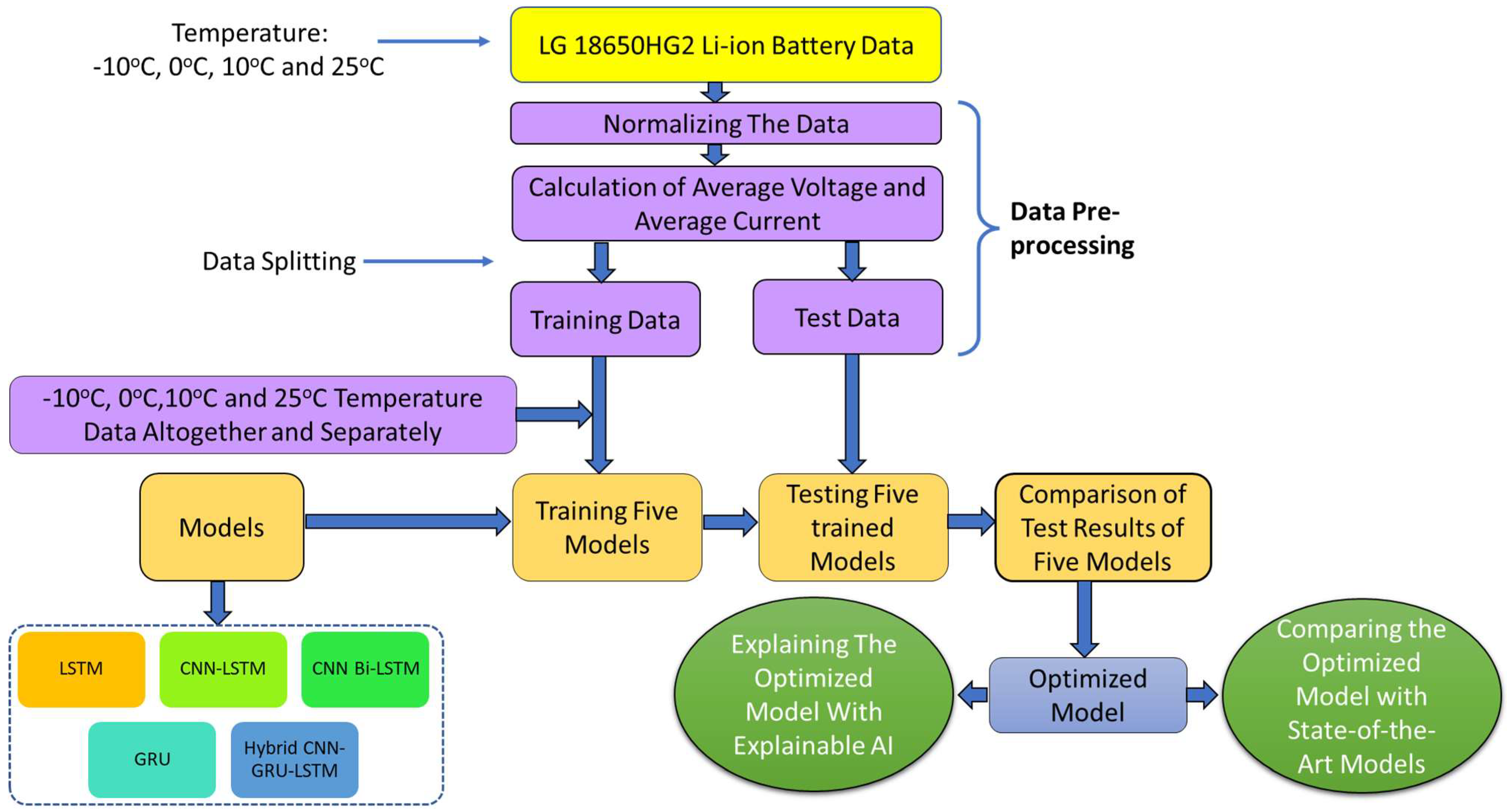
In this research, a hybrid CNN-GRU-LSTM (convolutional neural network-gated recurrent unit-long short-term memory network) model with an explainable AI, has been proposed, that can reliably and more accurately estimate the SOC while self-learning the network parameters, in order to contribute to the effective battery management for the EVs. The novel hybrid lightweight model was employed to minimize the SOC estimation error with a shorter processing time and a smaller memory use, due to a smaller number of parameters. The explainable AI would help to identify the most important feature from all of the input features for an accurate SOC estimation when the SOC data at different temperatures were used together and separately. The hybrid model was compared with four other models, such as the LSTM, CNN-LSTM, CNN-bi-directional LSTM, and GRU, to identify the best performing model. Furthermore, the performance of the hybrid model was compared with the state-of-the-art (SOTA) models to contribute to a better health management of the EV batteries.

The rest of the paper is organized as follows. Section 2 provides the materials and methods used in this paper to develop the model, while Section 3 discusses the models’ architecture. Section 4 presents the full experimental results and analysis. Finally, Section 5 draws conclusions, based on the findings.

2. Materials and Methods

2.1. Description of the Dataset

Data related to A LG 18650HG2 Li-ion battery [19] using a 3 Ah LG HG2 cell was used to train the RNN models. The Li-ion battery was tested in a 0.23 m³ thermal chamber and a 75 amp and 5 volt Digitron firing circuit was used as the battery tester. The test was conducted at six different ambient temperatures, ranging from −20 °C to 40 °C. A random combination of UDDS, HWFET, LA92, and US06, was used in a sequence of eight drive cycles (mix 1–8). In a compact electric car, the driving cycle power profile was computed for a single LG HG2 cell. Following each test, the battery was charged at a rate of 1C to 4.2 V with a 50 mA cutoff and a battery temperature of 22 °C or higher. The details of the test bench and the data logging system are given in [14].

The data of the four ambient temperatures (−10 °C, 0 °C,10 °C, and 25 °C) were chosen for this work. Four parameters, including voltage, current, temperature, and ampere-hour (Ah), were selected from the dataset to train the RNN models. The dataset was sampled to 1 Hz and the SOC was calculated by dividing the Ah data by the capacity of the battery cell. Then, two parameters were added to the dataset which were the average voltage and the average current determined by the moving window method. The sample data is shown in Figure 1.

2.2. Overall Design of the Study

The main objective of this work is to propose an optimized deep learning (DL) approach to estimate the SOC and explain the model with the explainable AI. The initial task was to collect and preprocess the data for the model training. Then five DL model architectures, based on CNN and RNN, were built to estimate the SOC of the EV battery in an optimum way. Then, these five models were trained with the training data and verified with the test data. A comparison was made among the models and an optimum model was selected. The optimum model performs better than the other four models, but does not state that it can be used in a BMS as a battery model. Therefore, the optimum model was also compared with the existing state-of-the-art models, and finally explained with an explainable AI and the feature importance was calculated using the SHAP library in Python. An overview of the workflow is shown in Figure 2.

2.3. Methodologies Used for the SOC Estimation

The RNN is one kind of artificial neural network (ANN) that is used in the analysis of sequential data. Nowadays, the RNN is used in the field of natural language processing (NLP), time series forecasting, voice recognition, and so on [20]. Since the SOC of a lithium-ion battery is estimated through the analysis of sequential data, the RNN can also be applicable here. Two types of RNN algorithms were used here: the long short-term memory (LSTM) and the gated recurrent unit (GRU). One dimensional convolution was also used for the feature extraction purpose from the data.

2.3.1. Long Short-Term Memory (LSTM)

The LSTM is specifically developed to prevent the problem of long-term dependency [20]. It is its default behavior to remember information for long periods of time. In Figure 3, c_k is denoted as the cell memory where k is denoted as time. The LSTM has three gates: forget, input, and output. The forget gate decides which information has to be erased from the cell memory and is defined by Equation (1) [14].

F_k = σ (w_f · [h_k−1, x_k] + b_f)

(1)

where, the sigmoid function, which is denoted by σ, is used and this provides the values of either 0 or 1. Mainly this sigmoid function decides whether the information in c_k−1 has to be erased or not. Here, w_f, h_k−1, x_k, and b_f, are weight metrics, previous layer hidden state vector, input vector, and the bias of the network, respectively.

The input gate keeps the new information in the unit memory c_k. The input gate is described by Equations (2) and (3).

i_k = σ (w_k · [h_k−1, x_k] + b_k)

(2)

c˜_k= tanh(w_c · [h_k−1, x_k] + b_c)

(3)

where the “input gate layer” i_k, which is built with a sigmoid layer, chooses which values have to be updated first. Following that, a tanh layer generates the c˜_k vector of the new candidate values that could be added to the state. Now, the outputs of Equations (1)–(3) are combined to update the unit memory c_k, defined by Equation (4).

c_k = f_k ∗ c_k−1 + i_k ∗ c_˜k

(4)

where, c_k is the unit memory. Now, the principle of the output gates will be discussed. The output has to be provided, based on the cell unit memory c_k. First, a sigmoid function is used to perform the task related to which part of the unit memory will be used, as the output (Equation (5)).

O_k = σ (w_o [h_k−1, x_k] + b_o)

(5)

where b_o is the bias. Now, the cell unit memory c_k is passed into a tanh function to make the values from −1 to 1. Then, it is multiplied by the output of the Equation (4) to obtain the output h_k (Equation (6)).

h_k = O_k ∗ tanh(c_k)

(6)

where h_k is the output. The main problem of the past RNN, was that previous inputs faded away with time. However, in the LSTM, the cell memory is controlled by the input and the forget gates. Thus, a long-term dependency problem is solved [21].

2.3.2. Gated Recurrent Unit (GRU)

Although the accuracy of the LSTM with three gates is very good, it is a complex model. Therefore, an updated version of the LSTM has emerged, and this is called the gated recurrent unit (GRU), which has an update gate and a reset gate. The reset gate controls how to integrate a new input with prior inputs in its memory, while the update gate specifies how much of the previous memory should be retained. The long-term dependencies can be explicitly modeled using this gating method. The network learns how its memory should function by learning the settings for its gates. Figure 4 explains the whole process in the GRU.

The reset gate is denoted by ‘r’ and the update gate is denoted by ‘z’. Equations (7)–(10) represent the whole GRU process [22]. The GRU reduces the complexity of the LSTM and works very well with small datasets.

z_k = σ (w_z · [h_k−1, x_k])

(7)

r_k = σ (w_r · [h_k−1, x_k])

(8)

h͂_k = tanh(w [r_k ∗ h_k−1, x_k])

(9)

h_k = (1 − z_k) ∗ h_k−1 + z_k ∗ h͂_k

(10)

where r_k is the reset gate and z_k is the update gate.

2.3.3. CNN for the Feature Extraction

A one-dimensional (1D) convolutional layer was used in this work. In a normal two-dimensional (2D) CNN, the kernels or filters stretch across both the spatial dimensions of an image, from left to right and from top to bottom. Moreover, the kernels in 1D-CNN layers only stretch in one dimension, which in this case is the temporal dimension. As a result, they can extract temporally relevant information [23]. The causal padding was used before running the filter. This is a unique sort of padding that mostly uses one-dimensional convolutional layers, that are particularly useful in time series analysis. As the time series provides the sequential data, it aids in the addition of zeros at the beginning and the prediction of the early time step values.

2.3.4. Explainable AI Tool

The explainable AI is a new feature of ML and DL that can explain a ML or DL model. In the process of ML or DL, at first, a model is trained with some input features and the outputs. Following the training of the model, if the input features are provided, the model provides an output result. However, the individual impact of the input features on the output is unknown. For example, in this SOC estimation model, if five inputs (voltage, current, temperature, average voltage, and average current) are provided, the model provides the SOC of the battery, but the model cannot determine the importance of each input feature, which can be explained by the explainable AI.

The Shapley Additive exPlanations (SHAP) is a library using Python, which is used to calculate the feature importance of a model. At first, SHAP takes a trained model, and with a sample dataset provided to SHAP, it makes predictions using the obtained dataset by shuffling the values in a single column. It calculates how much the loss function suffered from shuffling, using these forecasts and the true target values [24]. The importance of the variable just shuffled, is measured by the performance degradation. Then, it restores the data to its previous state (undoing the shuffle from step 2). Then, it repeats the step with the next column in the dataset, until it has computed the importance of all of the columns.

Lundberg and Lee’s recent work [25] on ML algorithms has created new ways to comprehend the model outputs. Based on the average of the geometrical contribution across all potential permutations of the features, the Shapley value is determined. The following mathematical expression is used for calculating the traditional SHAP value.

$${\varnothing }_j=\sum _{T\subseteq N\left\{j\right\}}\frac{\left|T\right|!(n-|T|-1)!}{n!}[f(T\cup \left\{j\right\})-f\left(T\right)]$$

(11)

where ∅_j stands for the contribution of feature j and N represents all features set. Then, n denotes the number of the features in set N, T is the subset of N that contains feature j and without knowing the feature values, the base value, or f(N), is the expected result for each feature in N. The SHAP value of each feature for a given observation, is added up to estimate the model result for that observation. As a result, the explanation model is defined by Equation (12).

$$g\left(z^{\prime }\right)={\varnothing }_0+\sum _{j=1}^M{\varnothing }_j{z}_j^{\prime }$$

(12)

where M is the features number and z′ is the input [26].

3. Architecture of the Employed Learning Networks

A total of five RNN models were employed for the SOC estimation. The models were built using TensorFlow, which is an open-source library that uses Python, and that is widely used in the field of ML and DL. These models were built, based on five types of layers, namely, a one-dimensional convolution layer, a LSTM layer, a bi-directional LSTM layer, a GRU layer, and a dense layer. Google Collab was used as the programming environment. The voltage, current, battery temperature, average voltage, and the average current were used as the input features and the SOC i% was used as the output. Adam was used as the optimizer, with the benefit of fixing the learning rate of the model itself [27]. An algorithm, regarding the whole process is given in Algorithm 1.

Algorithm 1. The model building and training method for the SOC estimation
Inputs	Voltage, Current, Temperature, Average Voltage, Average Current Input Shape = (5,1); Which corresponds (Number of Features, Window Size) Here, Number of Features = 5, Window Size = 1
Output	Five trained models and their performance parameters
Model Building	Building a model with just LSTM and dense layers Building a model with the addition of a one-dimensional convolution layer before the LSTM layers Building a model transforming the uni-directional LSTM layers into bi-directional. Building a model with just the GRU and dense layers Building a hybrid model with a one-dimensional convolution, and GRU and LSTM layers
Model Compiling	Defining the loss function as Mean Absolute Error (MAE) Defining the optimizer as “Adam”.
Training and Testing Models	Training the five models with training data and calculating the training errors. Testing the five models with test data and calculating the test error. (Errors are Mean Absolute Error, Root Mean Squared Error, and Maximum Error)

3.1. Learning Network 1: LSTM

Recurrent neural networks with a unique ability to disingenuously recognize sequences over extended periods of time, are known as long short-term memory (LSTM) networks. It is the best option for modeling sequential data and is therefore used to understand the intricate complexities of sentient behavior. The term “cell state” refers to the long-term memory. The preceding data is kept in the cells because of their recursive nature. Three LSTM layers with each layer consisting of 512 units, were added to the model. Then, a flatten layer was used to make the data three-dimensional to one-dimensional, followed by four dense layers, which have 1024, 1024, 512, and 128 units, respectively with the activation function “ReLU”. Finally, one dense layer of one unit was incorporated as the output layer. The architecture of the LSTM model is presented in Figure 5.

3.2. Learning Network 2: CNN-LSTM

The convolutional neural network (CNN) layers for the extraction of features on the input data are merged with the LSTMs, to endorse the sequential prediction in the CNN LSTM architecture. The CNN-LSTMs were created for concerns involving the prognostics of the visual time series, as well as the implementation of producing explanations from the visual patterns. The model architecture of the CNN-LSTM was almost same as the LSTM model with the key difference of a one-dimensional convolution layer, before the LSTM layers, which was added for the feature extraction purposes (Figure 6). It extracts the main features of the data before entering it into the LSTM layers. A total of 128 filters were used for the convolution process.

3.3. Learning Network 3: CNN-Bi-Directional LSTM

A bi-directional LSTM, also known as a Bi-LSTM, is a sequential computational framework, that consists of two LSTMs, one of which receives the input in forward time order, and the other receives the input in backward time order. The CNN-bi-directional LSTM architecture is almost the same as the CNN-LSTM model, except for the bi-directional LSTM layers, instead of the uni-directional LSTM layers, as shown in Figure 7. The rest of the architecture is the same. The input runs in two directions in a bi-directional LSTM. The input flows in one way, either backward or forwards, with the conventional LSTM. However, with the bi-directional LSTM, the information flows in both directions, preserving both the future and the past. When jobs requiring sequence to sequence are essential, the Bi-LSTM is typically used.

3.4. Learning Network 4: GRU

A gated recurrent unit (GRU) is a component of a particular type of recurrent neural network, that is designed to use the interconnection made through a series of nodes, to carry out machine learning activities involving memory and grouping, such as speech recognition. The main distinction between the GRU and LSTM, is that while the LSTM has three gates—input, output, and forget—the GRU only has two gates, update and reset. The GRU has fewer gates than the LSTM, making it less complicated. In the GRU model, three layers with each layer consisting of 64 units, were added in place of the LSTM layers, followed by a flatten layer and three dense layers with 1024, 1024, and 512 units with the activation function “ReLU”. Then, one dense layer with one unit was used as the output layer. The complexity of the GRU model is much less than that of the LSTM based models. The architecture of the GRU model is shown in Figure 8.

3.5. Learning Network 5: Hybrid CNN-GRU-LSTM

First, an explanation is needed why a CNN-GRU-LSTM hybrid model should be built. Although the LSTM is capable to solve the long-term dependency problems of the RNN and shows accurate results on large datasets, it needs more parameters and memory, in order to be executed, in contrast to the GRU. Hence, a combination of the LSTM and the GRU layers can provide the solution to the long-term dependency problem, but at the same time be less complex and less time-consuming.

At first, a one-dimensional convolution layer containing 128 filters was added for the feature extraction purpose, followed by a GRU layer of 64 units. Next, a LSTM layer of 64 units and a flatten layer were incorporated sequentially. Then, two dense layers, which have 1024 and 512 units, were added with the activation function “ReLU”. Finally, one dense layer of one unit was used as the output layer. The architecture of the CNN-GRU-LSTM hybrid model is shown in Figure 9.

3.6. Summary of the Learning Networks

The structural comparative analysis of the different learning network models is shown in

Table 1. Summary of the model characteristics.

Models	No. of Parameters	Model Depth (No. of Layers)	No. of CNN Layers	No. of RNN Layers	No. of Dense (Hidden) Layers
LSTM	9,513,729	7	0	3	4
CNN-LSTM	9,774,849	8	1	3	4
CNN Bi-LSTM	22,101,761	8	1	3 (Bi-directional)	4
GRU	1,729,217	6	0	3	3
CNN-GRU-LSTM	925,313	5	1	2	2

. According to the number of parameters and layers, the hybrid CNN-GRU-LSTM is the most lightweight model and the CNN-Bi-LSTM is the heaviest.

4. Quantitative Analysis and Validation of the Learning Networks

4.1. Performance Valuation Metrices

The mean absolute error (MAE), defined by Equation (13), was used as the loss function for training the model.

$$MAE=\frac{1}{N}{\displaystyle \sum }_{n=1}^N\left|SoC{\left(measured\right)}_k-SoC{\left(predicted\right)}_k\right|$$

(13)

where N is the length of the data. Following the training, the models were tested with the test data. The root mean squared error (RMSE) defined by Equation (14) and the maximum error defined by Equation (15) were chosen as the test criteria of the models, as well as the MAE.

$$RMSE=\sqrt{\frac{1}{N}{\displaystyle \sum }_{n=1}^N{\left(SoC{\left(measured\right)}_k-SoC{\left(predicted\right)}_k\right)}^2}$$

(14)

$$Max Error=MAX\left(\left|SoC\left(measured\right) – SoC\left(predicted\right)\right|\right)$$

(15)

4.2. Training with the Data of the Four Ambient Temperatures Altogether

In this experimental analysis, the data of all four ambient temperatures (10 °C, 0 °C, 10 °C, and 25 °C) were used collectively to train the five models with 669,956 training data.

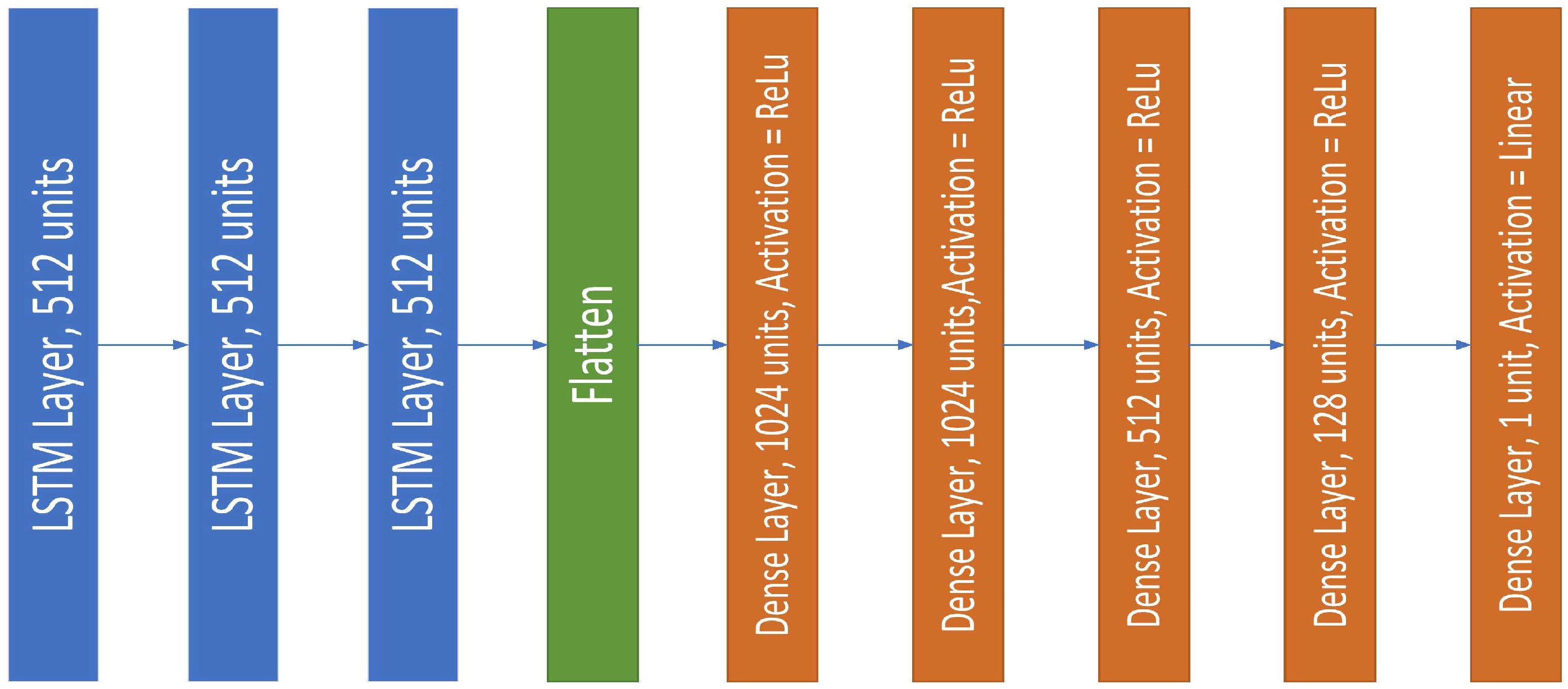
4.2.1. Training and Test Results of the LSTM Network

Following 15 epochs, the training mean absolute error (MAE) of the LSTM model was 0.93%. It took 55 min and 34 s for the whole training process with a total of 9,513,729 trainable parameters in the LSTM network. Following the training, the model was tested with the test data of the four ambient temperatures, separately, and the results are given in

Table 2. Test results of the LSTM model.

Temperature (°C)	Number of Test Data	Required Time (s)	MAE (%)	RMSE (%)	Max Error (%)
−10	39,293	4.03	0.79	1.11	4.17
0	42,530	4.12	0.64	0.89	4.65
10	44,284	4.26	0.90	1.56	8.43
25	47,517	5.14	0.87	1.10	4.50
Average			0.80	1.17	5.44

. The average MAE and RMSE of the LSTM model, based on the four ambient temperature data, were found as 0.81% and 1.17%, respectively. The remarkable point of the results was that no convolution layer was used for the feature extraction. Since the MAE was used as a loss function, the main goal of the training process was to reduce the MAE. The model performed best at 0 °C temperature where the MAE was only 0.64%, compared to the highest MAE of 0.9% at 10 °C.

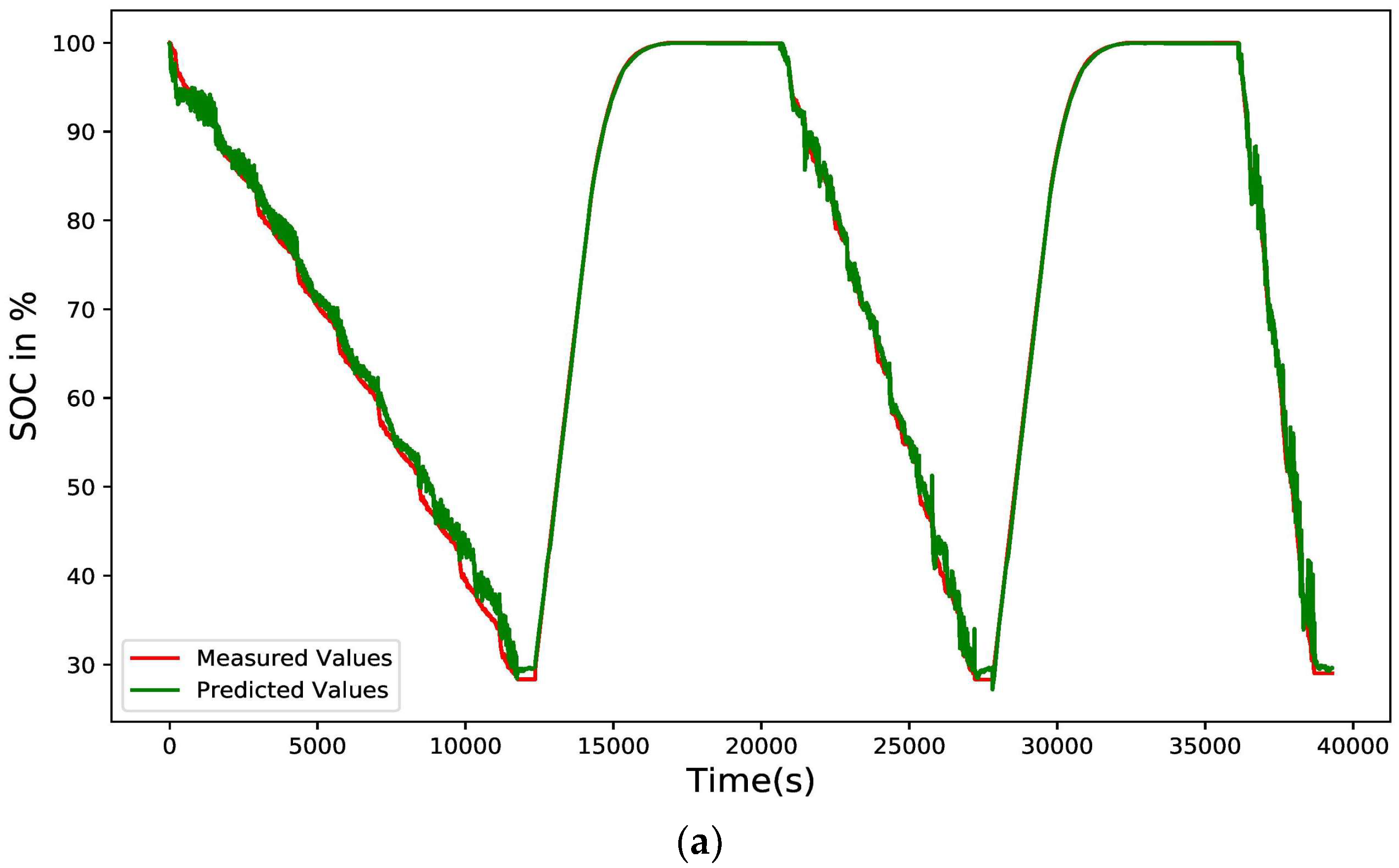
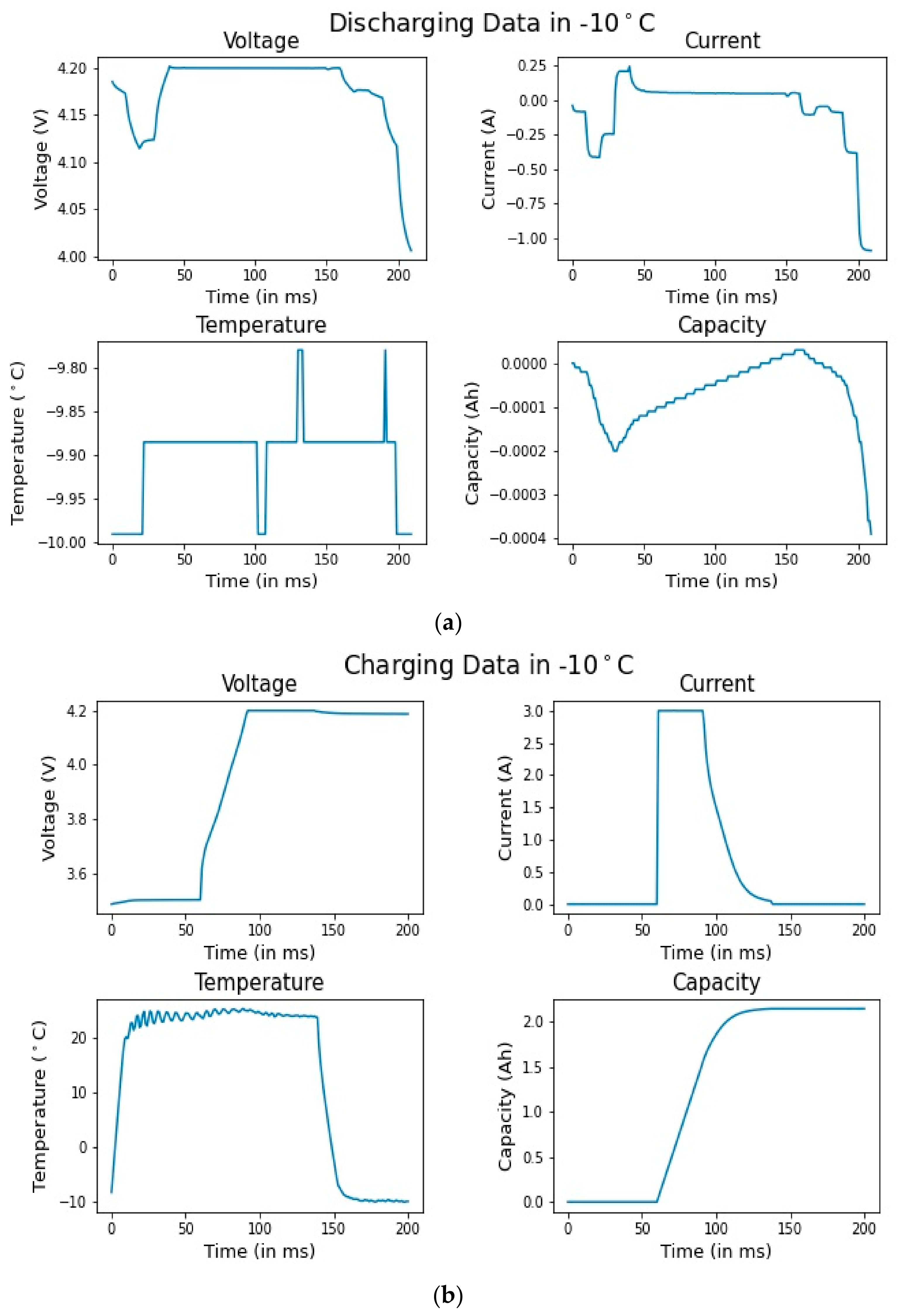
The plot of the measured and predicted SOC values of the LSTM model with the test data of −10 °C, is given in Figure 10a. Instead of plotting the data for all temperatures, the results of −10 °C is plotted as determining the SOC at lower ambient temperatures, is more critical than in higher temperatures [14,28]. From the graph, it was found that the model worked better with very small errors while charging, but generated more errors during the discharging process. Because of the experimental process, it is known that the battery was charged at a constant voltage process of 4.2 V. At the beginning of the charging process when the battery is empty, the current flow is normally higher. The current flow is subsequently decreased with the passage of charging time because the battery becomes gradually full of charge. Therefore, the charging process is quite simple, whereas discharging is not, as the battery is not discharged with a constant load, rather with the power profile of different drive cycles. When the battery is used in an electric vehicle, the load can be changed at almost every moment. Another remarkable phenomenon that happens during the discharging process is the regenerative braking, which is normally a charging process, where the loss of kinetic energy does not happen while braking, rather the energy is again stored in the battery. Therefore, the process of discharging is more complex making it very challenging to predict the accurate SOC while discharging, compared to the prediction of the SOC during the charging. This can be demonstrated by very smooth lines of the SOC during the charging process, compared to the noisy lines during the discharging process (Figure 10a). The plot of the absolute errors of the LSTM model on test data of −10 °C is shown in Figure 10b. The maximum error of the test data at −10 °C (4.17%), presented in Table 2, was also evidenced in Figure 10b. The error can be both positive and negative. As the optimization of the model was built, based on the mean absolute error, the absolute error is plotted for better understanding.

4.2.2. Training and Test Results of the CNN-LSTM Network

The CNN-LSTM network contained 9,774,849 trainable parameters and after 15 epochs, the training mean absolute error (MAE) was recorded as 0.91%, with 1 h 57 min and 24 s required for the whole training process. Adding a convolution layer with 128 filters, increased the training time by almost 1 h, reduced by 0.02% the training error, and increased a total of 261,120 trainable parameters. Following the training, the model was tested with the test data of the four ambient temperatures, separately, and the test results are shown in

Table 3. Test results of the CNN-LSTM model.

Temperature (°C)	Number of Test Data	Required Time (s)	MAE (%)	RMSE (%)	Max Error (%)
−10	39,293	10.12	0.82	1.23	9.30
0	42,530	11.04	0.70	1.12	9.28
10	44,284	12.10	0.89	1.65	8.37
25	47,517	13.40	0.49	1.00	11.50
Average			0.73	1.25	9.61

.

It was observed that the CNN-LSTM model showed a superior performance at 25 °C and a relatively poor performance at 10 °C. The average MAE and RMSE of the CNN-LSTM model, based on the four ambient temperature data, were 0.73% and 1.25%, respectively. Therefore, from the test result, it was clear that adding a convolution layer reduced the total mean absolute error, but the maximum error was increased. The testing time increased significantly, compared to the LSTM model because of the convolution layer, which extracted the feature from the data, and it is normally a time-consuming process. 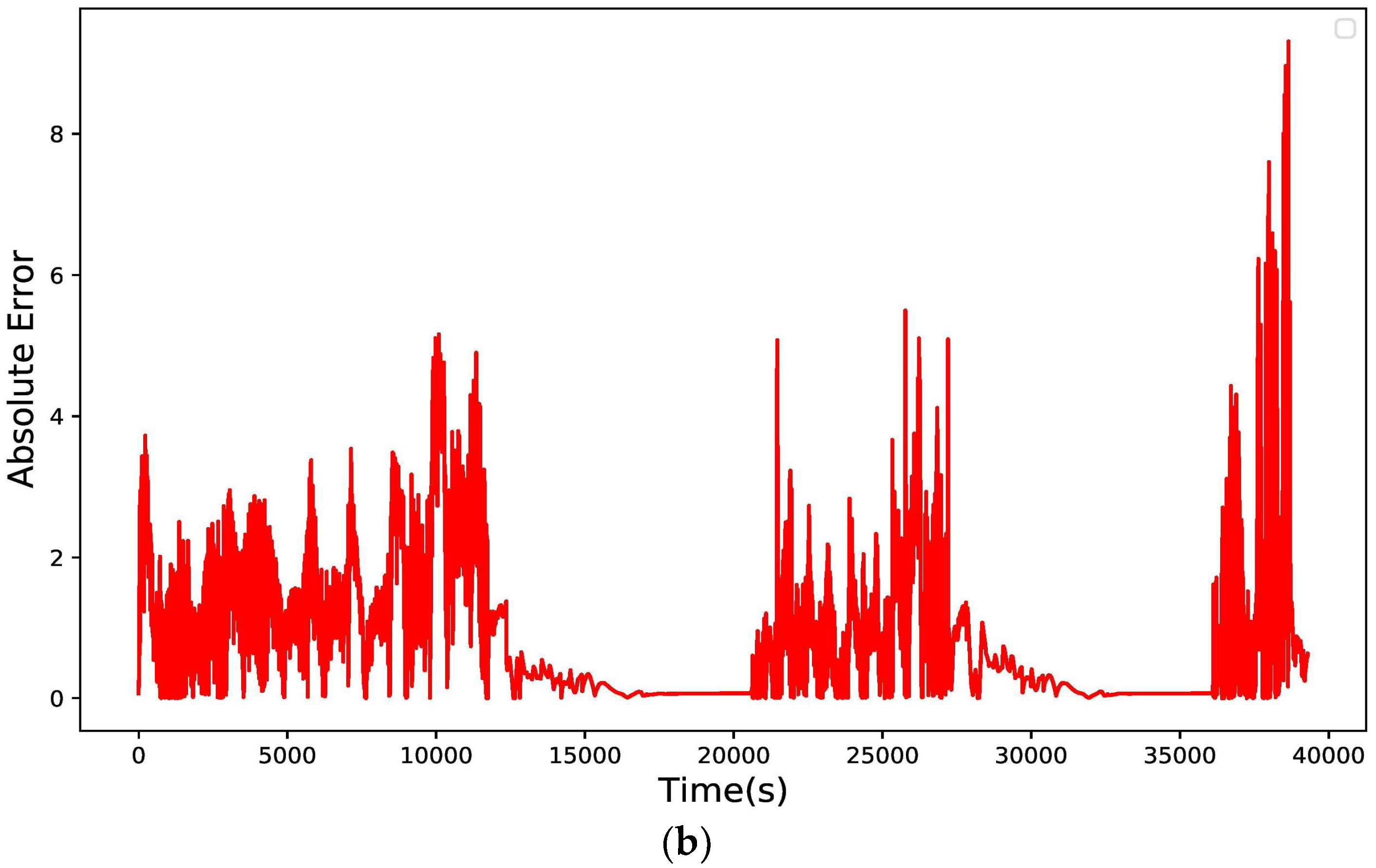The plot of measured values and predicted values of the CNN-LSTM model on the test data at −10 °C is presented in Figure 11a. The graph was also almost identical to the LSTM model performance graph with a better performance for the charging time SOC estimation, compared to that during the discharging. The absolute errors of the CNN-LSTM model on the test data at −10 °C is plotted in Figure 11b with a maximum error of 9.3%, which was higher than that of the LSTM model. It should be noted that only at a fewer points, were the error was so high. However, the overall test MAE of all of the temperature data of the CNN-LSTM model decreased to 0.73%, compared to 0.81% in the LSTM model. Therefore, though adding a convolution layer made the model more complex, the overall performance of the CNN-LSTM improved.

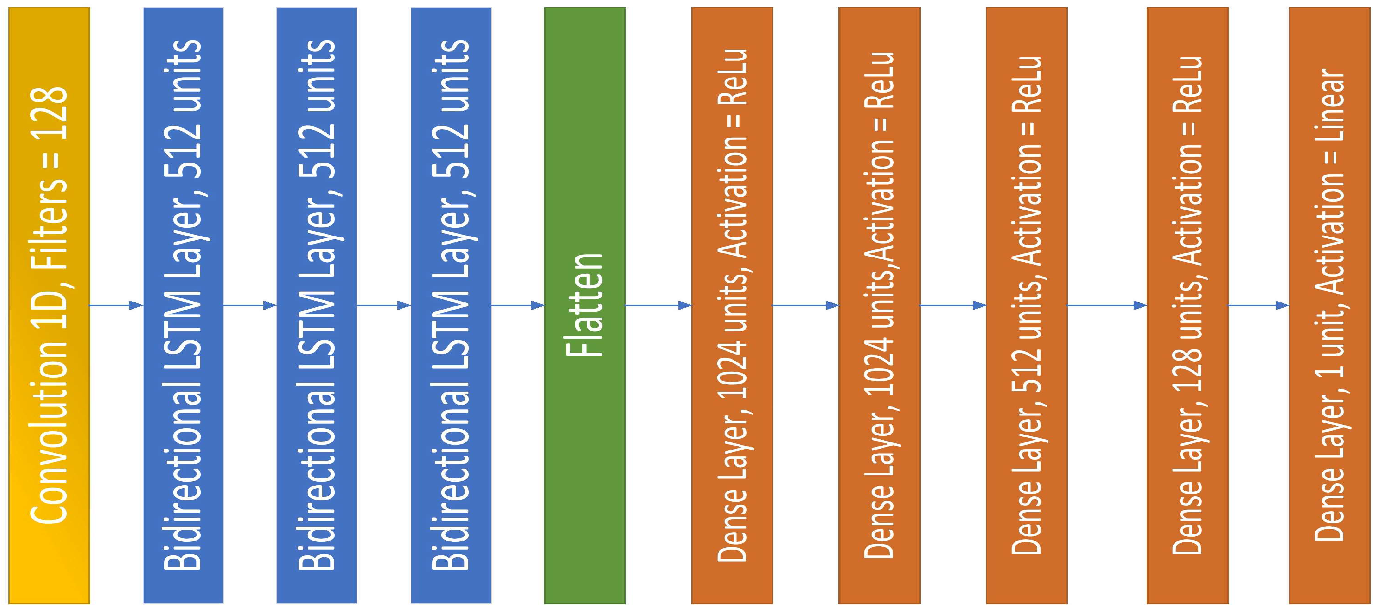
4.2.3. Training and Test Results of the CNN Bi-Directional-LSTM Network

During the CNN bi-directional-LSTM (CNN Bi-LSTM) model training, the MAE was found to be 0.87%, after running 15 epochs which took almost 3 h 55 min 32 s, which were about four and two times higher than the LSTM and CNN-LSTM models, respectively. The total number of 22,101,761 trainable parameters in the CNN Bi-LSTM model was more than double the previous two models. Adding the number of parameters means adding more complexity. Though the MAE was reduced by almost 0.04%, than that of the CNN-LSTM model, it required a huge amount of time for training. Therefore, this CNN Bi-LSTM model can be used where time and memory complexities are of minor importance, compared to the error. Following the training, the model was tested with the test data of the four ambient temperatures (

Table 4. Test results of the CNN bi-directional-LSTM model.

Temperature (°C)	Number of Test Data	Required Time (s)	MAE (%)	RMSE (%)	Max Error (%)
−10	39,293	20.52	0.64	1.05	5.23
0	42,530	20.52	0.67	0.97	5.78
10	44,284	20.29	0.89	1.62	8.00
25	47,517	21.75	0.55	1.07	9.11
Average			0.69	1.18	7.03

).

The average MAE and RMSE of the CNN Bi-LSTM model, based on the four ambient temperature data, were recorded as 0.69% and 1.18%, respectively, which were either similar to or better than the previous two models. Though it required more time to calculate the SOC, the error was on a satisfactory level. The testing time was almost double that of the CNN-LSTM model and four times greater than that of the LSTM model, possibly due to the bi-directional layers. In the normal uni-directional LSTM, the data passes in only the forward direction, whereas the data passes in both the forward and backward directions in the bi-directional layers. It was also observed that, similar to the CNN-LSTM model, the CNN Bi-LSTM model performed best at 25 °C and worst at 10 °C.

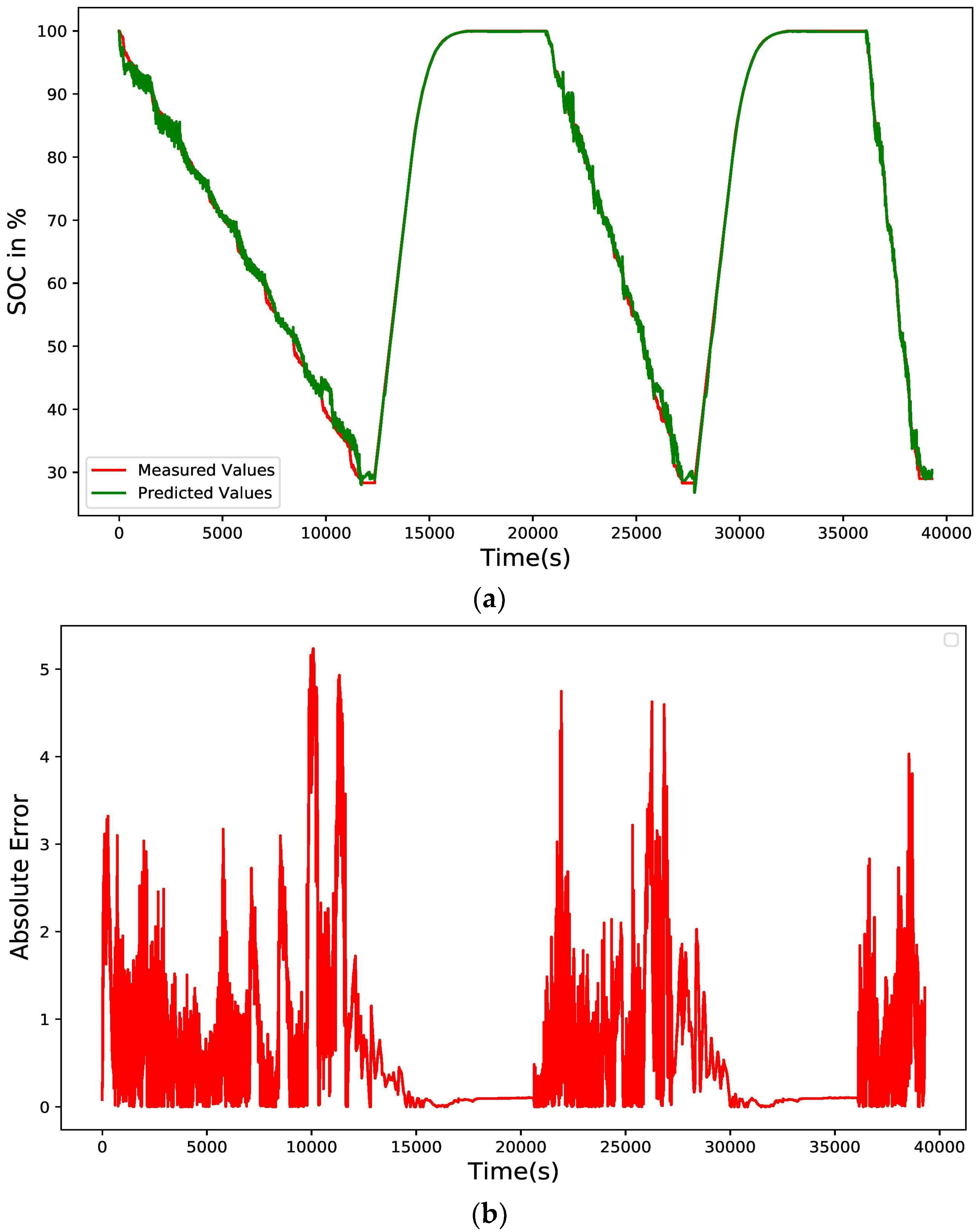
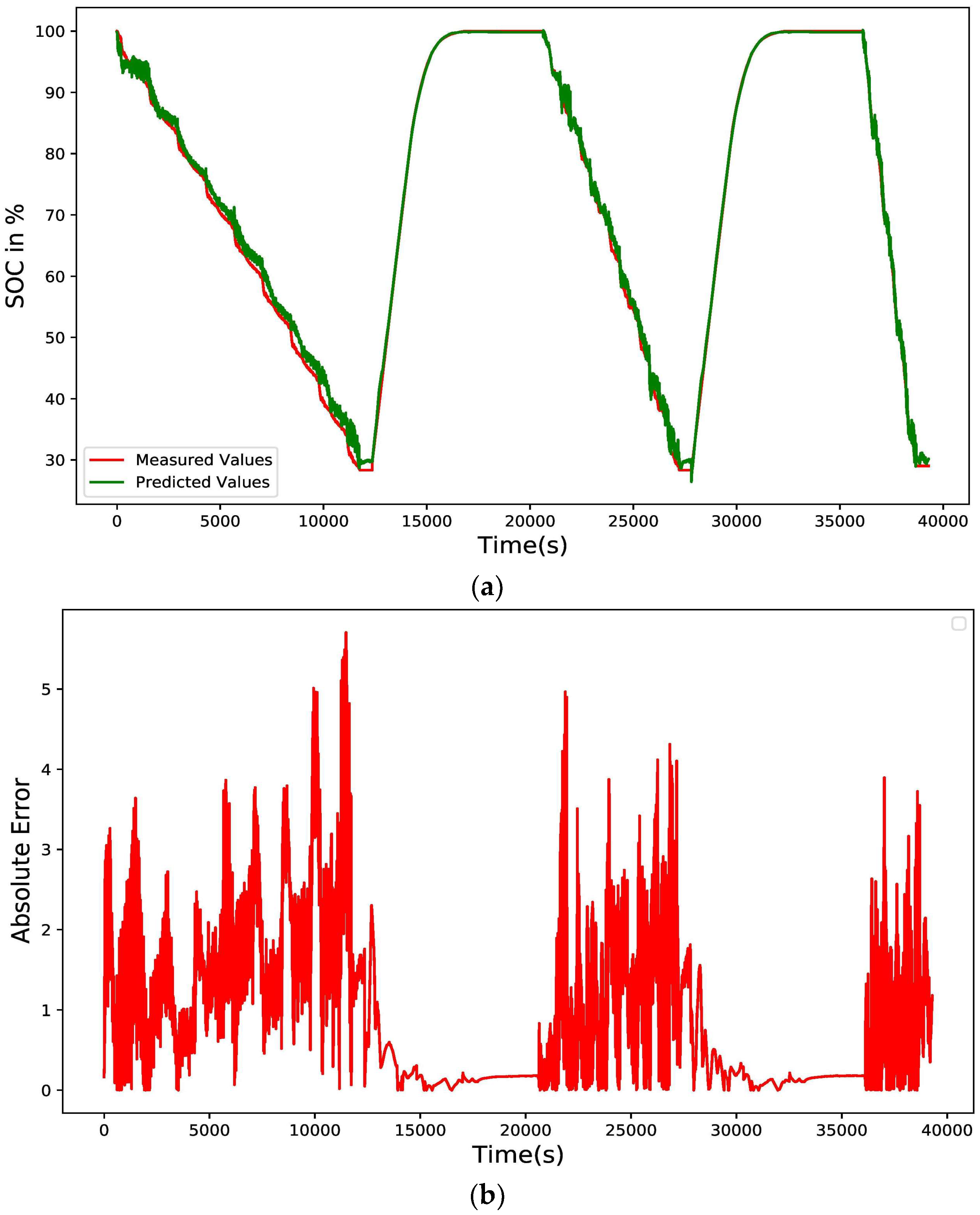
The plot of the measured values and predicted values of the CNN Bi-LSTM model, based on the test data at −10 °C during the charging and discharging, showed a similar trend to that of the previous models (Figure 12a). From Figure 12b and Table 4, a maximum error value of 5.23% was found for the CNN Bi-LSTM model on the test data at −10 °C, which was in between the previous two models. The overall lower MAE of the CNN Bi-LSTM model indicated a sign of a better performance than the previous two models.

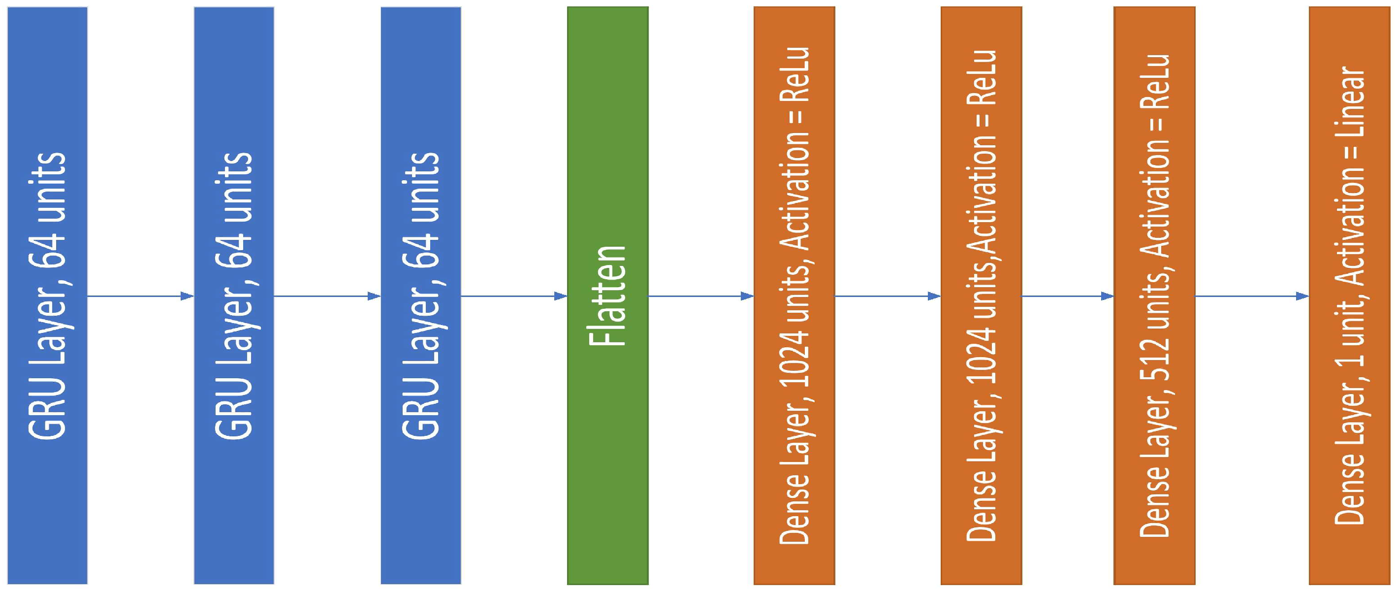
4.2.4. Training and Test Results of the GRU Network

For the GRU model, after 15 epochs, a MAE of 0.88% was found, which took almost 1 h 29 min and 45 s for the training, with a total of 1,729,217 trainable parameters. The GRU is a more lightweight model than the LSTM, with a smaller number of parameters than the three previous LSTM-based models. Based on the similarity, the GRU model architecture was similar to the LSTM model. The main difference identified was that the three layers of the LSTM model had 512 units, compared to the 64 units in the GRU model, indicating that it is less complex than the LSTM model. The CNN Bi-LSTM showed a very good performance in predicting the SOC but with the shortcomings of the complex model, a longer calculation time, a high number of parameters, and a larger memory space. Therefore, the optimization can be carried out using the GRU model instead of the LSTM models, as it achieved almost the same training error as the CNN Bi-LSTM model. The test results of the GRU model are presented in

Table 5. Test results of the GRU model.

Temperature (°C)	Number of Test Data	Required Time (s)	MAE (%)	RMSE (%)	Max Error (%)
−10	39,293	5.15	1.17	1.58	8.34
0	42,530	5.13	0.76	1.05	7.13
10	44,284	5.11	1.19	2.00	10.36
25	47,517	5.71	0.94	1.48	10.12
Average			1.02	1.53	8.99

.

The average MAE and RMSE of the GRU model, based on the four ambient temperature data, were found as 1.02% and 1.53%, respectively. Though a smaller training error was found in the GRU model, the test results were poorer than the LSTM models. Some sort of over fitting was observed in the test results of the GRU model, but the testing time was smaller due to it being a lightweight model.

From Table 5, the GRU model performed well at 0 °C and the highest errors were found at 10 °C. The absolute error results on the test data at −10 °C can be observed in Figure 13a. Overall, the GRU model could not predict the SOC as correctly as the LSTM based models, but the complexity and testing times of the model were reduced with a reduction of the trainable parameters. When the GRU model was compared to a similar type, such as the LSTM model, which showed a 0.2% less MAE than the GRU model because the LSTM model performed better with large datasets. The absolute error graph of the GRU model on the test data at −10 °C (Figure 13b) showed that the max error of 8.34% was present only at one point, while at other points, all absolute error values were below 6%.

4.2.5. Training and Test Results of the Hybrid CNN-GRU-LSTM Network

In order to take advantage of the best functional features of the individual models, a hybrid CNN-GRU-LSTM network was proposed. For reaching the optimized point, the GRU layer reduced the complexity and the LSTM layer made the necessary steps to obtain a better result in the large dataset. Moreover, the CNN layer carried out the feature extraction task very well.

Upon the completion of 15 epoch runs, a MAE of 0.82% was achieved with the total trainable parameters of 925,313 in the hybrid CNN-GRU-LSTM network. It was very lightweight, compared to the other four models, due to the one GRU layer and the one LSTM layer, while the other models have three LSTM or GRU layers. Other LSTM-based models had 512 units in every layer, in contrast to the 64 units in the hybrid model. Though it had a smaller number of parameters, it showed a better training performance than the other four models, with least amount of training time (53 min and 22 s). The MAE and the training time were both improved in this hybrid model. The test results for the hybrid model are given in

Table 6. Test Results of the hybrid CNN-GRU-LSTM model.

Temperature (°C)	Number of Test Data	Required Time (s)	MAE (%)	RMSE (%)	Max Error (%)
−10	39,293	5.15	0.86	1.30	5.70
0	42,530	5.16	0.61	1.00	4.80
10	44,284	4.31	0.90	1.62	11.50
25	47,517	5.01	0.63	1.00	9.80
Average			0.75	1.23	7.95

.

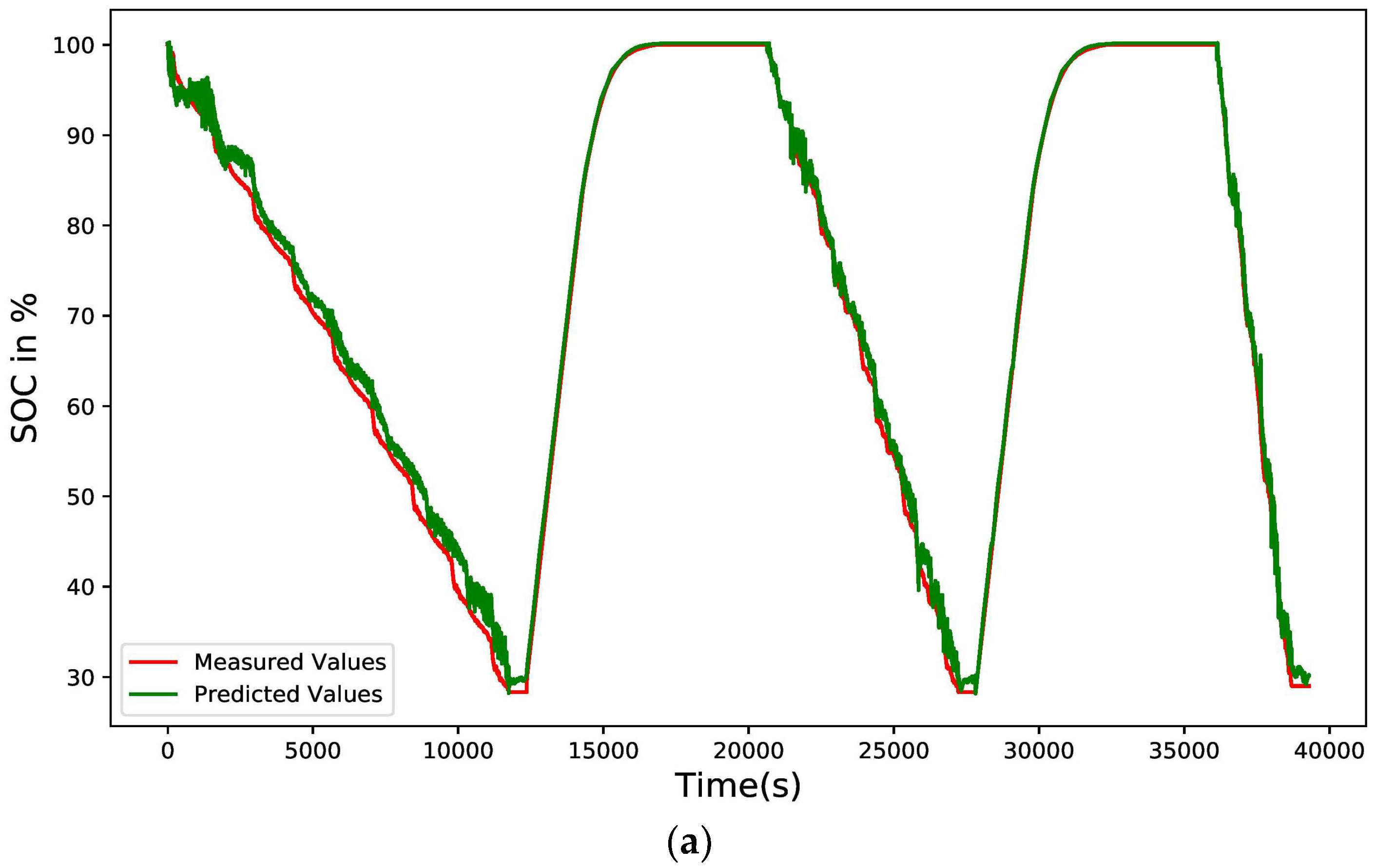
The average MAE and RMSE of the hybrid CNN-GRU-LSTM model, based on the four ambient temperature data, were recorded as 0.75% and 1.23%, respectively, which were similar to the LSTM based models but better than the GRU model with a smaller number of layers and units. The test results and the absolute errors of the hybrid CNN-GRU-LSTM model on the test data of −10 °C can be observed in Figure 14a and Figure 14b, respectively. The model performed best at 25 °C and worst at 10 °C.

4.2.6. Comparative Analysis among the Five Models

It is highly important to choose an optimized model for the SOC of a lithium-ion battery management system, which will be governed by model error, prediction time, and number of trainable parameters. A higher error obviously reduces the prediction accuracy, which is undesirable. As well, as the SOC is used in the battery energy management of an electric vehicle, a longer prediction time to calculate the SOC would slow down the BMS response. Furthermore, a higher number of trainable parameters would increase the size of the model and hence the memory requirement.

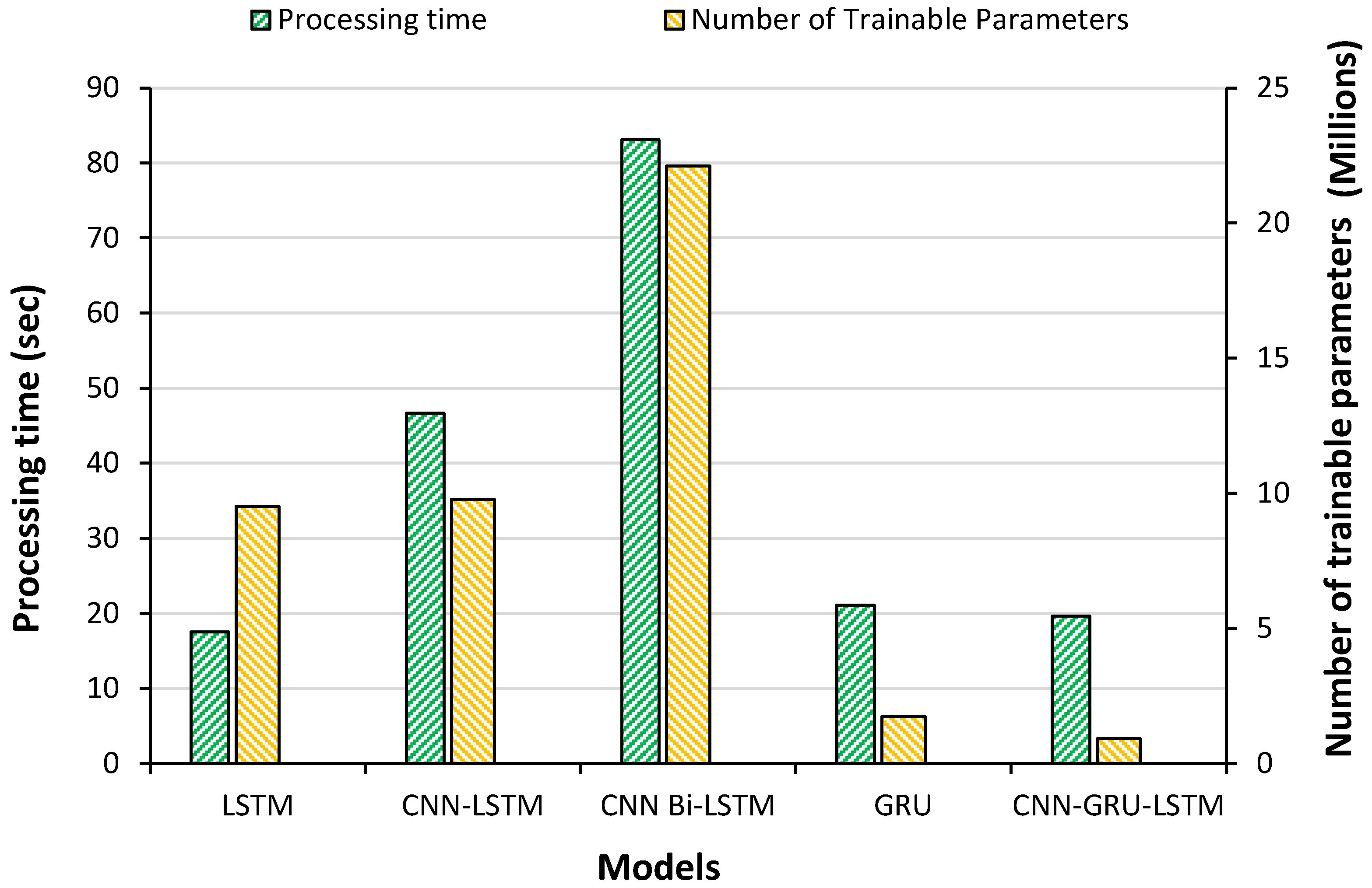
All of the five models tested in this work, performed quite well, hence it is challenging to select the best model, as almost every model performed better than the others with the test data obtained at any particular temperature. A comparison was made with the overall error, prediction time, and number of trainable parameters, and presented in Figure 15 and Figure 16.

It was clear from the graphs that the CNN Bi-LSTM determined the SOC most correctly, but its prediction time and number of trainable parameters were the highest among the tested models. However, the hybrid CNN-GRU-LSTM showed almost the same errors as the CNN-LSTM model, but its prediction time and number of trainable parameters were either equal to or smaller than the other models. Therefore, the hybrid model could be considered as the optimum one among the five models tested.

4.3. Training with the Data of the Four Ambient Temperatures Separately

It is also important to train the optimum hybrid model with separate temperature data, to determine its performance. Following the training with the separate temperature data, the training MEAs were found as 0.42%, 0.46%, 0.38%, and 0.35%, for −10 °C, 0 °C, 10 °C, and 25 °C, respectively, where the 0.82% training MAE was found while training with all of the temperature data altogether. Therefore, it can be concluded that if the models are developed with the data obtained at the different ambient temperatures separately, the error can be reduced.

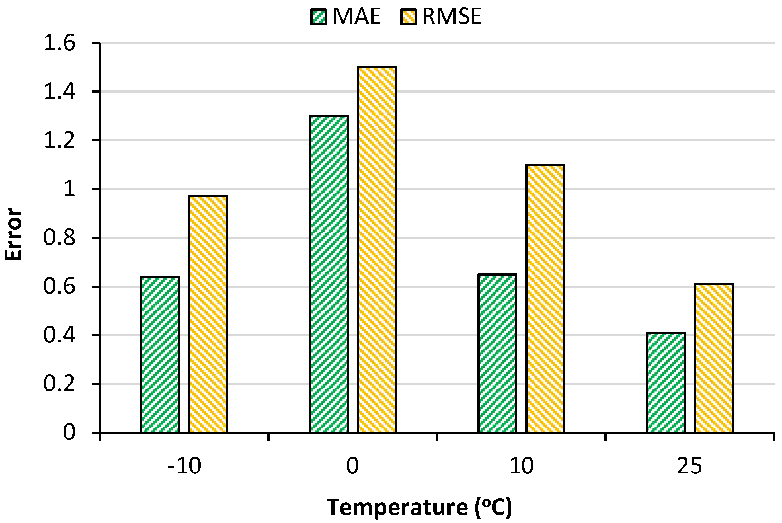
Following the training, the model was tested with the test data and the results are shown in

Table 7. The test result when the CNN-GRU-LSTM model is trained using separate temperature data.

Temperature (°C)	MAE (%)	RMSE (%)	Max Error (%)
−10	0.64	0.97	6.25
0	1.30	1.50	5.80
10	0.65	1.10	7.60
25	0.41	0.61	4.20

and Figure 17. The best performance was obtained for the model developed with the data at 25 °C. The higher error at 0 °C could be due to an increase in the battery’s internal resistance [14].

4.4. Comparative Analysis with the State-of-the-Art (SOTA) Models

The hybrid CNN-GRU-LSTM model was also compared with other SOTA models, reported in the literature, using the performance parameters including the MAE and RMSE (

Table 8. Comparative analysis for the five studies.

Type of Model	Temperature Data Use	Ambient Temp. (°C)	MAE (%)	Lithium-Ion Battery Specification	Reference
LSTM-RNN	Together	0 10 25	2.088 0.782 0.774	Panasonic 2.9 Ah NCR18650PF	[14]
	Fixed	10 25	0.807 0.68%
DNN	Together	−20 −10 0 10 25	0.22 1.4 0.9 1.9 1.1	Panasonic 2.9 Ah NCR18650PF	[28]
	Fixed	25	0.61
Extreme Learning Machine	Together	25	<1.5 MAX	Samsung 2.6 Ah	[29]
Adaptive Unscented Kalman Filter with Support Vector Machine	Together	25 to 42	<2.0	Kokam 70 Ah	[30]
Sunflower Optimization Algorithm Extended Kalman Filter	N/A	10 25 40	1.24 0.82 1.37	LG 18650HG2 3 Ah	[31]
Hybrid CNN-GRU-LSTM	Together	−10 0 10 25	0.86 0.61 0.90 0.63	LG18650HG2 3 Ah	Current study
	Fixed	−10 0 10 25	0.64 1.30 0.65 0.41

). Chemali et al. [14] proposed a LSTM-RNN model that could predict the SOC. However, this LSTM-RNN network had 1000 units in the hidden layer. They found their best result while training their model with the fixed temperature data at 25 °C which was 0.68% of the MAE. Chemali et al. [28] proposed a deep neural network (DNN) approach and obtained their best result of a 0.61% MAE at 0 °C. A Panasonic 2.9 Ah NCR18650PF battery was used in these two proposals. Du et al. in [29] proposed an extreme learning machine battery model, which can estimate the SOC under a maximum error of 1.5%, when the test was performed with a Samsung 2.6 Ah battery. Meng et al. [30] proposed an adaptive unscented Kalman filter with a support vector machine to calculate the SOC using a Kokam 70 Ah battery, and achieved the SOC under a 2% MAE. Maheshwari et al. [31] proposed the sunflower optimization algorithm extender Kalman filter method and determined the SOC from 0.82% to 1.37%of the MAE on a LG 18650HG2 3 Ah dataset.

The hybrid CNN-GRU-LSTM model proposed in this work achieved only a 0.41% MAE at a 25 °C ambient temperature, in contrast to the lowest error of a 0.61% MAE at 25 °C, found in the previous works. At −10 °C and 10 °C ambient temperatures, 0.64%, and 0.65% MAE errors were found, respectively. At 0 °C temperature, a 0.61% MAE was found when the model was trained with the four temperature data altogether. Therefore, with the 25 °C temperature data, the model performed best, which reduced by almost 0.2% the MAE from the previous work. At −10 °C, 0 °C, and 10 °C, the performance was also better than the previous studies and the proposed hybrid model was lightweight and less complex than the others. For instance, even the best performing LSTM-RNN model [14] had 1000 hidden units in the hidden layers, compared to only 64 hidden units in the hybrid model. Therefore, it can be concluded that the proposed hybrid model can outperform the SOTA models.

4.5. Explaining the Hybrid CNN-GRU-LSTM Model with the Explainable AI

4.5.1. Model Trained with the Four Ambient Temperature Data Altogether

The Python SHAP library was used to determine the feature importance. At first, the model that was trained with the data altogether, was tested with SHAP and presented in Figure 18, which revealed that, from the five inputs, the average voltage was the most important input feature. The prediction of the SOC depends on the average voltage the most and on the nonlinear behavior of the battery voltage. Since the average voltage is the average of the voltages (the present voltage and the previous voltage values) of a moving window, which is a statistical method to quickly identify the changes in the residual mean value and standard deviation [32], it contains a lot of information on the previous condition of the SOC. It is the main requirement of the RNN, that the previous important input and output, should be considered for the present output. Following the average voltage, the present voltage is another important input feature. As the average voltage contains information about the previous and present states altogether, the instantaneous voltage information is also an important feature for the SOC estimation. Furthermore, the average current containing the information on the present and previous loads on the battery, is also important information for the SOC estimation. As the battery behavior changes with the ambient temperature, its importance is shown in the SHAP chart. The instantaneous current was shown to be a less important feature, as its impact was very low in the SOC estimation. Therefore, the CNN-GRU-LSTM model could detect the input feature importance from the dataset on the SOC estimation more correctly, based on SHAP values.

4.5.2. Models Trained with Separately with the Four Ambient Temperature Data

The feature importance graph, based on the models trained on the four ambient temperatures separately is shown in Figure 19. The top important features at all four temperatures, sequentially, were identified as average voltage, voltage, and average current, though the value of the importance (SHAP value) were variable at different temperatures. The least important features (current and battery temperature) altered their positions between 4th and 5th places. If the importance of temperature was observed, it was noticed that the most impact was made on the model trained with the data of 10 °C. Therefore, the temperature could be placed at the 4th position before the current, in terms of the feature importance. However, in the other three models, the position of the feature importance of the temperature was 5th, and current was 4th. The model trained with 25 °C data showed temperature as the least important feature. The trained model with 0 °C and −10 °C data, the temperature showed some importance as a feature.

Now, further analysis is required to understand the importance of the input features. The models that were trained with the four temperature data altogether, the temperature feature importance was high possibly due to the fact that the SOC behavior of the battery was constantly changing with the change of temperature. However, when the model was trained with the data of the four temperatures separately, the temperature was the least important feature in three circumstances out of four. This could be explained by the fact that, when the model was trained with the data of the same ambient temperature, the battery behavior was remained constant.

4.6. General Discussion

The diversity of battery advancements will increase, due to the high demand for EVs, and as all types of batteries have distinct electrical and chemical constituents and functionalities, this will create a great deal of instability and provide difficulties for a comprehensive SOC estimation.

The proposed hybrid CNN-GRU-LSTM battery model can estimate the SOC with a very little amount of error, which is very helpful for the BMS of EVs because, the SOC is very significant and critical information for the BMS and the EV driver. Since the proposed battery model is very lightweight, it will consume a very small amount of memory in the BMS and the SOC estimation time will be very short, which will help the BMS to respond faster. Another feature of this work is the novel hybrid model of the LSTM and GRU layers, where two RNN layers have been used. The LSTM units are more accurate than the GRU in the long dataset, but two LSTM layers would increase the complexity of the model. Therefore, one LSTM layer and one GRU layer were used, which ensured both the accuracy and lightweightedness of the model. The hybrid CNN-GRU-LSTM model can estimate the SOC consuming less memory in the BMS, with the least calculation time and the least amount of error, which are the key qualities of an ideal battery model for a BMS.

The existing studies focused on estimating the SOC but it is still unknown which input features are more important in the SOC estimation. The determination of the input feature importance is a novel and crucial aspect of this work, as it can add a new dimension to the development of the BMS. Since, the average voltage and voltage are the most important input features, more precision while measuring the battery voltage will enhance the BMS performance. Moreover, since the average voltage was measured using the moving window method, an increment of the size of the moving window will boost up the accuracy of the SOC. From the description of the dataset, the data (voltage, current, and temperature) were collected at the sample rate of 1 Hz. From the input feature importance bar chart, the voltage is a more important input feature than the current and temperature. Therefore, the sample rate of the voltage can be increased, while implementing the battery model to the BMS.

5. Conclusions

The study proposed a hybrid CNN-GRU-LSTM network to predict the SOC of lithium-ion batteries in the most optimized way. A total of five RNN models (LSTM, CNN-LSTM, CNN Bi-LSTM, GRU and CNN-GRU-LSTM) were built, trained, and tested to identify the optimum model, by comparing the performance parameters, such as the error values, prediction time, and number of trainable parameters. The SOC is very important and vital information for the BMS and the EV driver, and the proposed model can estimate it with a very small amount of error (best result: 0.41% MAE at 25 °C), which is very helpful for the BMS of the EVs. Two RNN layers were used in this model’s LSTM and GRU layers. In the lengthy dataset, the LSTM units were more accurate than the GRU, but adding two LSTM layers would make the model more complex. Therefore, one LSTM layer and one GRU layer were used, guaranteeing the model’s accuracy and portability. The hybrid CNN-GRU-LSTM model has the key characteristics of the perfect battery model for a BMS as it can estimate the SOC while using less memory (11,170,968 bytes) in the BMS, with the least amount of calculation time (0.000113 s/sample), and with the least amount of error.

This hybrid CNN-GRU-LSTM model, demonstrated to be a robust tool for battery management systems, as it estimated the SOC correctly, within the shortest amount of time and consumed a small amount of memory in the BMS. When all of the temperature data (−10 °C, 0 °C, 10 °C, and 25 °C) were used together, the MAE ranged between 0.61% to 0.90%. Furthermore, the MAE values were with the range of 0.41% to 1.3% when the temperature data was used separately. The hybrid model used the least number of input parameters (925,313) and consumed the least amount of processing time (training time and testing time), when compared to the other models. The explainable AI has identified the average voltage as the most influential parameter, in order to accurately estimate the SOC. This brings a new dimension to effectively manage the EV battery system.

The hybrid model reduced the MAE by 0.20% over the existing best battery model, with the least number of parameters, which outperforms the existing models. It produced a 32.79% better accuracy than the existing models in the literature. The number of units was also reduced in this hybrid model, compared to other existing work, as it made the hybrid model more lightweight. In future, the most optimum model for determining the State of Health (SoH) and State of Energy (SoE) will be proposed. Moreover, the BMS has some special requirements for machine learning-based SOC computational methods. For example, the BMS should have a powerful CPU/GPU for receiving a fast response. The future task would be focused on reducing the computational burdens.

References

1. Espedal, I.B.; Jinasena, A.; Burheim, O.S.; Lamb, J.J. Current trends for state-of-charge (soc) estimation in lithium-ion battery electric vehicles. Energies 2021, 14, 3284. [Google Scholar] [CrossRef]
2. Macioszek, E. Electric Vehicles—Problems and Issues. In Smart and Green Solutions for Transport Systems; TSTP 2019; Sierpiński, G., Ed.; Advances in Intelligent Systems and Computing; Springer: Berlin/Heidelberg, Germany, 2020; Volume 1091. [Google Scholar] [CrossRef]
3. Ling, Z.; Cherry, C.R.; Wen, Y. Determining the Factors That Influence Electric Vehicle Adoption: A Stated Preference Survey Study in Beijing, China. Sustainability 2021, 13, 11719. [Google Scholar] [CrossRef]
4. Macioszek, E. E-mobility infrastructure in the Górnośląsko-Zagłębiowska Metropolis, Poland, and potential for development. In Proceedings of the 5th World Congress on New Technologies (NewTech’19), Lisbon, Portugal, 18–20 August 2019; pp. 1–4. [Google Scholar] [CrossRef]
5. Misyris, G.S.; Doukas, D.I.; Papadopoulos, T.A.; Labridis, D.P.; Agelidis, V.G. State-of-charge estimation for li-ion batteries: A more accurate hybrid approach. IEEE Trans. Energy Convers. 2018, 34, 109–119. [Google Scholar] [CrossRef] [Green Version]
6. Okay, K.; Eray, S.; Eray, A. Development of prototype battery management system for pv system. Renew. Energy 2022, 181, 1294–1304. [Google Scholar] [CrossRef]
7. Lipu, M.H.; Hannan, M.; Karim, T.F.; Hussain, A.; Saad, M.H.M.; Ayob, A.; Miah, M.S.; Mahlia, T.I. Intelligent algorithms and control strategies for battery management system in electric vehicles: Progress, challenges and future outlook. J. Clean. Prod. 2021, 292, 126044. [Google Scholar] [CrossRef]
8. Chang, W.-Y. The state of charge estimating methods for battery: A review. Int. Sch. Res. Not. 2013, 2013, 953792. [Google Scholar] [CrossRef] [Green Version]
9. Xiong, R.; Cao, J.; Yu, Q.; He, H.; Sun, F. Critical review on the battery state of charge estimation methods for electric vehicles. IEEE Access 2017, 6, 1832–1843. [Google Scholar] [CrossRef]
10. Darbar, D.; Bhattacharya, I. Application of machine learning in battery: State of charge estimation using feed forward neural network for sodiumion battery. Electrochem 2022, 3, 42–57. [Google Scholar] [CrossRef]
11. Vidal, C.; Kollmeyer, P.; Naguib, M.; Malysz, P.; Gross, O.; Emadi, A. Robust xev battery state-of-charge estimator design using a feedforward deep neural network. SAE Int. J. Adv. Curr. Pract. Mobil. 2020, 2, 2872–2880. [Google Scholar]
12. Hannan, M.A.; Lipu, M.S.H.; Hussain, A.; Saad, M.H.; Ayob, A. Neural network approach for estimating state of charge of lithium-ion battery using backtracking search algorithm. IEEE Access 2018, 6, 10069–10079. [Google Scholar] [CrossRef]
13. Wang, Q.; Wu, P.; Lian, J. Soc estimation algorithm of power lithium battery based on afsa-bp neural network. J. Eng. 2020, 13, 535–539. [Google Scholar] [CrossRef]
14. Chemali, E.; Kollmeyer, P.J.; Preindl, M.; Ahmed, R.; Emadi, A. Long short-term memory networks for accurate state-of-charge estimation of li-ion batteries. IEEE Trans. Ind. Electron. 2017, 65, 6730–6739. [Google Scholar] [CrossRef]
15. Bian, C.; He, H.; Yang, S. Stacked bidirectional long short-term memory networks for state-of-charge estimation of lithium-ion batteries. Energy 2020, 191, 116538. [Google Scholar] [CrossRef]
16. Jiao, M.; Wang, D. The savitzky-golay filter based bidirectional long short-term memory network for soc estimation. Int. J. Energy Res. 2021, 45, 19467–19480. [Google Scholar] [CrossRef]
17. Yang, F.; Li, W.; Li, C.; Miao, Q. State-of-charge estimation of lithium-ion batteries based on gated recurrent neural network. Energy 2019, 175, 66–75. [Google Scholar] [CrossRef]
18. Jiao, M.; Wang, D.; Qiu, J. A gru-rnn based momentum optimized algorithm for soc estimation. J. Power Sources 2020, 459, 228051. [Google Scholar] [CrossRef]
19. Kollmeyer, P.; Vidal, C.; Naguib, M.; Skells, M. Lg 18650hg2 li-ion battery data and example deep neural network xev soc estimator script. Mendeley Data 2020, 3. [Google Scholar] [CrossRef]
20. Naguib, M.; Kollmeyer, P.; Vidal, C.; Emadi, A. Accurate surface temperature estimation of lithium-ion batteries using feedforward and recurrent artificial neural networks. In Proceedings of the 2021 IEEE Transportation Electrification Conference & Expo (ITEC), Chicago, IL, USA, 21–25 June 2021; pp. 52–57. [Google Scholar]
21. Yang, F.; Zhang, S.; Li, W.; Miao, Q. State-of-charge estimation of lithium-ion batteries using lstm and ukf. Energy 2020, 201, 117664. [Google Scholar] [CrossRef]
22. Zhao, R.; Kollmeyer, P.J.; Lorenz, R.D.; Jahns, T.M. A compact unified methodology via a recurrent neural network for accurate modeling of lithium-ion battery voltage and state-of-charge. In Proceedings of the 2017 IEEE Energy Conversion Congress and Exposition (ECCE), Cincinnati, OH, USA, 1–5 October 2017; pp. 5234–5241. [Google Scholar]
23. Bhattacharjee, A.; Verma, A.; Mishra, S.; Saha, T.K. Estimating state of charge for xev batteries using 1 d convolutional neural networks and transfer learning. IEEE Trans. Veh. Technol. 2021, 70, 3123–3135. [Google Scholar] [CrossRef]
24. Zhang, K.; Xu, P.; Zhang, J. Explainable ai in deep reinforcement learning models: A shap method applied in power system emergency control. In Proceedings of the 2020 IEEE 4th Conference on Energy Internet and Energy System Integration (EI2), Wuhan, China, 30 October–1 November 2020; pp. 711–716. [Google Scholar]
25. Lundberg, S.M.; Lee, S.-I. A unified approach to interpreting model predictions. In Advances in Neural Information Processing Systems; 2017; p. 30. Available online: https://proceedings.neurips.cc/paper/2017/file/8a20a8621978632d76c43dfd28b67767-Paper.pdf (accessed on 24 October 2022).
26. Dikshit, A.; Pradhan, B. Interpretable and explainable AI (XAI) model for spatial drought prediction. Sci. Total Environ. 2021, 801, 149797. [Google Scholar] [CrossRef]
27. Peyal, H.I.; Shahriar, S.M.; Sultana, A.; Jahan, I.; Mondol, M.H. Detection of tomato leaf diseases using transfer learning architectures: A comparative analysis. In Proceedings of the 2021 International Conference on Automation, Control and Mechatronics for Industry 4.0 (ACMI), Rajshahi, Bangladesh, 8–9 July 2021; pp. 1–6. [Google Scholar]
28. Chemali, E.; Kollmeyer, P.J.; Preindl, M.; Emadi, A. State-of-charge estimation of li-ion batteries using deep neural networks: A machine learning approach. J. Power Sources 2018, 400, 242–255. [Google Scholar] [CrossRef]
29. Du, J.; Liu, Z.; Wang, Y. State of charge estimation for li-ion battery based on model from extreme learning machine. Control. Eng. Pract. 2014, 26, 11–19. [Google Scholar] [CrossRef]
30. Meng, J.; Luo, G.; Gao, F. Lithium polymer battery state-of-charge estimation based on adaptive unscented kalman filter and support vector machine. IEEE Trans. Power Electron. 2015, 31, 2226–2238. [Google Scholar] [CrossRef]
31. Maheshwari, A.; Nageswari, S. Real-time state of charge estimation for electric vehicle power batteries using optimized filter. Energy 2022, 254, 124328. [Google Scholar] [CrossRef]
32. Guo, P.; Bai, N. Wind turbine gearbox condition monitoring with AAKR and moving window statistic methods. Energies 2011, 4, 2077–2093. [Google Scholar] [CrossRef]
Figure 1. Sample data plot for the measured parameters of the terminal voltage, current, temperature, and battery capacity (Ah) while (a) discharging and (b) charging the battery at −10 °C.
Energies 15 08003 g001
Figure 2. Overall design of the study for the SOC estimation of the EV battery.
Energies 15 08003 g002
Figure 3. The internal architecture of a LSTM unit containing all of the parameters and gates.
Energies 15 08003 g003
Figure 4. The internal architecture of a GRU containing all of the parameters and gates.
Energies 15 08003 g004
Figure 5. Architecture of the LSTM model.
Energies 15 08003 g005
Figure 6. Architecture of the CNN-LSTM model.
Energies 15 08003 g006
Figure 7. Architecture of the CNN bi-directional-LSTM model.
Energies 15 08003 g007
Figure 8. Architecture of the GRU model.
Energies 15 08003 g008
Figure 9. Architecture of the hybrid CNN-GRU-LSTM model.
Energies 15 08003 g009
Figure 10. Performance of the LSTM model at −10 °C (a) measured and predicted SOC values and (b) absolute errors from the test data.
Energies 15 08003 g010
Figure 11. Performance of the CNN-LSTM model at −10 °C (a) measured and predicted SOC values and (b) absolute errors from the test data.
Energies 15 08003 g011aEnergies 15 08003 g011b
Figure 12. Performance of the CNN bi-directional-LSTM model at −10 °C (a) measured and predicted SOC values and (b) absolute errors from the test data.
Energies 15 08003 g012
Figure 13. Performance of the GRU model at −10 °C (a) measured and predicted SOC values and (b) absolute errors from the test data.
Energies 15 08003 g013aEnergies 15 08003 g013b
Figure 14. Performance of the hybrid CNN-GRU-LSTM model at −10 °C (a) measured and predicted SOC values and (b) absolute errors from the test data.
Energies 15 08003 g014
Figure 15. MAE and the RMSE of the five RNN models.
Energies 15 08003 g015
Figure 16. Comparison of the models with respect to the processing time and trainable parameters.
Energies 15 08003 g016
Figure 17. MAE and the RMSE of the CNN-GRU-LSTM model in the four different temperatures.
Energies 15 08003 g017
Figure 18. Feature importance of the hybrid CNN-GRU-LSTM model trained with the four temperature data altogether.
Energies 15 08003 g018
Figure 19. Feature importance of the hybrid CNN-GRU-LSTM model trained with the data of (a) −10 °C (b) 0 °C, (c) 10 °C and (d) 25 °C.
Energies 15 08003 g019