Article

Modeling of Magnetic Properties of Rare-Earth Hard Magnets

1
Chair of Physics, Częstochowa University of Technology, 42-201 Częstochowa, Poland
2
Department of Semiconductors and Optoelectronics Devices, Łódź University of Technology, 90-924 Łódź, Poland
3
Chair of Electric Power Engineering, Częstochowa University of Technology, 42-201 Częstochowa, Poland
*
Authors to whom correspondence should be addressed.
Energies 2022, 15(21), 7951; https://doi.org/10.3390/en15217951
Submission received: 28 September 2022 / Revised: 20 October 2022 / Accepted: 24 October 2022 / Published: 26 October 2022

Abstract

:
Magnetic properties of hard magnets are currently attracting a great deal of attention. In the paper, the modified Harrison model was used to describe the saturating hysteresis loops of three praseodymium–dysprosium ribbons that differed in their chemical composition and processing conditions. Microstructural studies (TEM and diffraction patterns) were performed for the ribbons under consideration. The Harrison model incorporates a number of physically tangible concepts such as the anhysteretic curve, bifurcations, and bi-stability. The modification of the original approach consisted of adding an additional degree of freedom in the modeling by freeing the restraints present in the original version, in which both coercivity and remanence are functions of temperature only.

Graphical Abstract

1. Introduction

1.1. Basic Information on Magnetic Materials

Magnetic materials may be classified as soft, semi-hard and hard. The figure of merit used for this distinction is the coercivity value, i.e., the value of the field strength that has to be applied to the material in order to reduce the magnetic induction (or magnetization) to zero. For soft magnetic materials, one usually neglects the difference between the intrinsic coercivity Hci (defined as the field strength at which the magnetization is reduced to zero) and normal coercivity Hc (defined as the field strength at which the induction is reduced to zero). Typically, the coercivity values for soft magnetic materials do not exceed 1 kA/m. At the other extreme are hard magnetic materials, for which the values of intrinsic coercivity exceed 10 kA/m [1]. Semi-hard materials (carbon or cobalt steels are examples thereof) usually exhibit coercivities that range from 1 kA/m to 10 kA/m. The upper limit is somewhat arbitrary since some materials such as AlNiCo or Remalloy may be considered as either semi-hard or hard; the distinction is made depending on their application scope [2].
Hard magnetic materials are sometimes referred to as permanent magnets since they maintain constant magnetic properties once they are magnetized. They exhibit a large hysteresis loop area (which represents the energy dissipated as heat if the material is subject to re-magnetization in alternating magnetic fields). Figure 1 depicts the difference between the shape of the hysteresis loop for a soft and a hard magnetic material.

1.2. Hard Magnetic Materials—Examples of Applications and Their Recovery from e-Waste

Hard magnetic materials have a wide range of applications in various industries, for example:
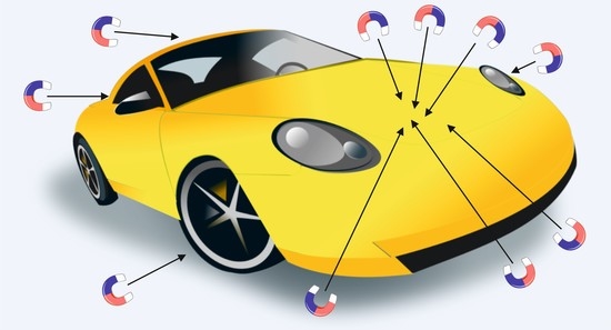
  • Automotive: motors, alternators, control systems, anti-lock braking systems (ABS), audio systems (loudspeakers), as shown in Figure 2, which depicts just a few specific examples;
  • Computer science: hard disk drives, actuators, printers;
  • Consumer electronics and home appliances: washing machines, induction cookers, microwave ovens, audio systems, refrigerators, radios and television;
  • Electronics: sensors, electro-mechanical transducers, contactless switches;
  • Mechatronics: brushless DC motors, permanent magnet synchronous motors;
  • Telecommunication: microphones, loudspeakers, switches and relays;
  • Medicine: magnetic resonance imaging (MRI) and nuclear magnetic resonance spectroscopy (NMR), surgery;
  • Power engineering: wind turbines;
  • Aerospace and aviation: gauges, fuel pumps, position and speed sensors, rotor assemblies, air compressors, cryogenic magnets for space, magnetic levitation systems.
A recent discussion on the state-of-the-art status of permanent magnets, their properties and cost-related issues may be found in [4]. Based on the above-given compilation, it follows that hard magnetic materials play a crucial role in the everyday life of humans. The range of applications for permanent magnets is constantly increasing; however, there are significant problems related to the depletion of natural resources and possible shortages, in particular, of rare-earth (RE) metals [5]. Thus, in recent years a great deal of attention has been paid to the issue of how to limit the use of permanent magnets, e.g., in the automotive industry [6,7] or power engineering [8,9], and how to recover rare earth metals and other precious elements from waste electrical and electronic equipment (WEEE) [10,11,12,13,14]. The European Commission has also focused on the latter problem [15]. Each year, International E-Waste Day is held on 14 October to promote the correct disposal of e-waste. As noted quite recently on theregister.com website [16], it is estimated that of the 16 billion mobile phones owned worldwide, around 5.3 billion will become e-waste in 2022. In 2022 alone, small EEE items such as cell phones, electric toothbrushes, toasters and cameras produced worldwide will weigh an estimated total of 24.5 million tons—four times the weight of the Great Pyramid of Giza. These small items make up a significant proportion of the 8% of all e-waste thrown into trash bins and eventually landfilled or incinerated. On the other hand, junk cellphones and other waste electronic equipment contain significant amounts of RE metals, which can be recovered and re-used.

1.3. Hysteresis Models Used in Electrical Engineering

The modeling of hysteresis loops might be useful at the design stage of devices containing magnetic circuits. In engineering practice, two approaches have attracted considerable interest, namely, the phenomenological Preisach description [17] (later scrutinized by Mayergoyz [18] and Della Torre [19]) and the macroscopic Jiles–Atherton model [20]. The research on hysteresis modeling has focused primarily on soft magnetic materials since the abundance of possible output states for arbitrary input signal variations for these materials, e.g., during transient states, makes the prediction problem interesting and at the same time important for practical applications (for example, the precise tripping of protection systems during surges in power engineering) [21].
Models of the hysteresis loops for hard magnets are thus less common than for soft magnetic materials, as usually only a reliable description of the major (saturating) loop is needed, possibly supplemented with a description of the first-order reversal curves (cycles starting from arbitrary points on the descending branch of the major loop, in hard magnet terminology referred to as recoil curves). Most of the existing models for hard magnets are derived from the Jiles–Atherton model [22,23,24,25]; however, several other alternatives have become available recently [26,27].
Table 1 presents a comparison of several hysteresis models, which are considered by the authors as the most widely used and as particularly useful in electrical engineering.
Several of the physical assumptions that underlie the Jiles–Atherton formalism have been questioned. The authors of [65] criticized the decomposition of total magnetization into irreversible and reversible components, present in one of the fundamental equations of the Jiles–Atherton model, as deprived of physical interpretation. Moreover, they pointed out that the application of the “effective field” as the argument for the “anhysteretic” magnetization in the modified Langevin function leads to an S-shaped curve passing through the second and the fourth quadrants of the M–H plane (if implicitly anhysteretic magnetization appears on both sides of the Langevin relationship) or to the appearance of a hysteresis loop for the anhysteretic curve itself (which contradicts its physical meaning), an exemplary modeled curve can be found in [66]. Rather, the energy balance equation of Jiles and Atherton resembles a summation of co-energy terms; thus, the model is deprived of physical meaning.
The issue of the energy balance equation in the Jiles–Atherton model was revisited in [67]. The authors analyzed several versions of the Jiles–Atherton model equation and modified the model assumptions inherent in the original Jiles’ derivation. The modification allowed them to improve the modeling accuracy for higher order reversal curves.
Since there are some problems with the physical assumptions of the Jiles–Atherton formalism, in this contribution we focus on the modification of an alternative model developed by Harrison [29]. The consistency of the latter model with the Landau [68] theory of phase transitions was highlighted recently in [49]. The Harrison approach, in spite of its simplicity, which might suggest a “toy model”, is based on a profound physical interpretation and it offers a thermodynamically consistent description of the magnetization process.
In the Harrison model, there is a distinction between the irreversible and reversible contributions and the outcome hysteresis loop is the result of their summation at the domain scale; however, there are significant differences between this formalism and the Jiles–Atherton model. Briefly, there is no feedback in the description for the anhysteretic curve, which behaves correctly from a thermodynamic point of view (it passes monotonously only through the first and third quadrant of the M–H plane, and exhibits saturation). In the framework of the Harrison model, the anhysteretic curve results primarily from domain wall pinning [29], which is contrary to statements by Jiles and Atherton, who claim that domain wall pinning results in hysteresis.
The original paper by Harrison [29] suggests the wide applicability of his formalism. There are several exemplary modeling results for Nd2Fe14B and SmCo5 hard magnets; however, the reference curves were taken from a textbook [1]. The aim of the paper was to verify the model using real-life measurement data. In order to improve its accuracy we introduced some additional degrees of freedom to the model. We analyzed the chosen relationships between the modified model parameters and the magnetic properties given for hysteresis loops of praseodymium–dysprosium ribbons annealed at different rates.

2. Materials and Methods

Ingot samples with a nominal composition of Pr8Dy1Fe60Co7Ni(6−x)MnxB14Zr1Ti3 (where x = 0, 3, 6) were prepared by arc melting in a protective argon atmosphere with high purity elements with a known Fe-B admixture. The samples were melted repeatedly to obtain homogeneity. The ribbons were then produced using single-roll melt spinning in the argon atmosphere. The linear speed of the copper wheel surface used in this process was 30 m/s. The completely amorphous ribbon samples were then sealed in a quartz tube under low argon pressure to keep the atmosphere clean during the heat treatment. In order to obtain the nanocrystalline microstructure, the samples were annealed at various temperatures ranging from 923 K to 1023 K for 5 min, and then quickly cooled in water.
The hysteresis loops of the three ribbons prepared from praseodymium–dysprosium compounds were measured using a Vibrating Sample Magnetometer VSM7307 from Lakeshore (Woburn, MA, USA) (see Figure 3 and Figure 4) for external magnetic fields up to 2 T.
For modeling purposes, the samples with the best magnetic parameters were selected. The basic magnetic information (coercivity—JHC, remanence—Jr, saturation polarization—Js and the product of maximum energy—(BH)max) for the tested samples is provided in Table 2.
The obtained parameters indicate that all of the analyzed samples are magnetically hard. The coercivity ranges from 563 kA/m for an alloy without Mn and increases with the addition of manganese (790 kA/m for an alloy containing 3 at.% of Mn) to 986 kA/m for an alloy in which all the Ni has been replaced with Mn. An enhancement in the remanence (Jr/Js > 0.5) was found in all the tested alloys, which suggests the occurrence of exchange-coupling in the ribbons.
The microstructural characterization of the ribbons was performed with the use of transmission electron microscopy. The TEM pictures were collected using the Hitachi STEM HD2700 (Tokyo, Japan). Figure 5 and Figure 6 depict the TEM micrographs at different zoom levels and the corresponding diffraction patterns for Sample 1 and 3, respectively. These revealed the non-homogeneous microstructure of the samples with small grains embedded in an amorphous matrix. This fact was confirmed with XRD studies [69]. The microstructure of the samples containing manganese contained finer grains, in the range of 20–30 nm.

3. Modeling

Let us recall the constitutive relationship between magnetic induction B, polarization J (or magnetization M) and magnetic field strength H, which are valid for both soft and hard magnets. B = μ 0 H + J = μ 0 ( H + M ) , where μ 0 = 4 · π · 10 7 H/m is the free space permeability. Polarization J is expressed in Teslas, which is the same as magnetic induction B; however, it has saturation properties, and therefore both curves differ significantly for hard magnets [1]. The curves presented in Figure 4 clearly exhibit saturation. In the present paper, we prefer to work with magnetic polarization J than with magnetization M (the first part of the expression above, using the Kennelly notation [1]), since its magnitudes are of unit order. In some expressions, the dimensionless units are used, then the reduced polarization is equivalent to the reduced magnetization.
For the Harrison model, it is expedient to treat the magnetic field strength H as the output of a “black box” representing the hysteresis operator since this formalism belongs to the class of the so-called inverse models [49].
We considered the following set of model equations.

3.1. The Reversible Curve

In the first approximation, we assume that the description of the reversible (anhysteretic) curve may be given with the Cohen approximation [70] of the inverse Langevin function
H an = γ   j   3 j 2 1 j 2
where γ   ,   MA/m is a fitting parameter, whereas j = J / J s stands for the reduced polarization (referred to as the saturation value).
In the original Harrison approach, the model developer used numerical methods to invert the Langevin function whereas in our paper we prefer to provide an analytical equation. The computation of the inverse Langevin function still attracts the attention of numerous researchers. Several representative examples include the recent studies in [71,72,73,74,75,76,77,78]; thus, our choice is somewhat arbitrary. However, we note that this simple description has just one fitting parameter; moreover, its Maclaurin expansion yields 3 γ  j as its first term, which can be immediately recognized as the reciprocal of the Maclaurin expansion for the Langevin function j = coth H / γ γ / H   since lim H 0 d j / d H = 1 / ( 3 γ ) .
The anhysteretic curve, which describes the state of global thermodynamic equilibrium, may be recovered for soft magnets using a tedious process that relies on the repetitive application of a decaying signal for successive values of the bias field. For hard magnets, the situation is even more complicated. Therefore, we followed the approach outlined in the “classic” textbook by Bozorth [79], which was further examined, e.g., by Krah and Bergqvist [80] and de Souza Dias et al. [49]. In this approach, we considered the “measured” anhysteretic curve as the connected set of points determined as the middle curve from the ascending and the descending branches of symmetric hysteresis loops. Thus, our approach is based on the assumption that there is a correspondence between the shapes of the hysteresis loop and of the anhysteretic curve, as postulated by Takács [35].
Figure 7 depicts the fitting of the reconstructed “measured” anhysteretic curves to the Cohen relationship (1). The values of saturation polarization were fixed to those given in Table 1. Table 3 includes the estimated values of the γ parameter that appears in (1). The fitting results were only in qualitative agreement with the experiment.
However, much better modelling results were obtained when the saturation magnetization was freed from the preset values and treated as the second fitting parameter, see Figure 8. For the latter case it can be stated that generally, good accuracy was achieved (the worst, yet still acceptable, fitting results were obtained for Sample 2). Table 4 includes the estimated values of the γ and J s parameters.
We also checked the other modeling options, namely, the application of the area hyperbolic tangent function to describe the anhysteretic curve H an = H an ( J ) . Both Langevin and the hyperbolic tangent function are used extensively in solid state physics and they are the limiting cases for the Brillouin function, corresponding either to isotropic or highly anisotropic magnetic properties [80]. Higher discrepancies between the reconstructed and modeled curves were found more consistently than in the previous case, therefore we have not reported them.
At this point, we can draw the following conclusions:
  • The measured values for saturation polarization reported in Table 2 are higher than their modeled counterparts. The assumption that the true saturation polarization values in the samples may differ from the nominal ones improves the modeling results, as shown in Figure 6. However, we assumed a tolerance of 10% of the value reported in Table 2 only, so that the physical meaning of parameter γ might be retained.
  • Thus, the values reported in Table 2 should be treated as indicators for the first approximation only.
  • The trend for the modeled values of saturation polarization is consistent with the trend reported in Table 2.
  • The estimated value of the fitting parameter γ is the highest for the sample 1 and the lowest for sample 3, if we assume that both γ and J s are free fitting parameters.
  • It is tempting to make conclusions about the microstructural properties of the examined samples (that they are isotropic rather than anisotropic, since the inverse Langevin function yields better results than the area hyperbolic tangent); however, the modeling accuracy cannot be treated as a sufficient for drawing meaningful conclusions about the morphology of the samples, and it should be supported with in-depth material characterization studies.

3.2. The Irreversible Curve

In the original Harrison model, an algebraic equation is used to describe the S-shaped curve related to the description of the irreversible processes until the so-called bifurcation points are reached. At these points, steep vertical magnetization “jumps” to the other loop branch are envisaged (this is an example of the so-called catastrophe, see [81] for details), taking into account reversible curve leads to the realistic shapes of loop branches [29]. In the model, the loop branches are “glued” from distinct line segments, which makes the analysis somewhat difficult.
Thus, the Harrison description takes both the irreversible and reversible components of magnetic field strength into account. However, their summation cannot be simply undertaken for any arbitrary value of polarization (magnetization) because if the threshold value at the bifurcation point is reached, it is “latched” until the loop branches intersect.
In the original Harrison model, the S-shaped curve, whose parts form the purely irreversible loop, is given with a self-consistent relationship (here written in dimensionless units):
j = tanh h + j t
where j is the reduced polarization, h is the reduced field strength and t is the reduced temperature. After the transformations, one obtains the following relationship for the h = h (j) coordinate system
h = t atanh j j .
Equation (3) is very important for the theory, since its direct differentiation with respect to j, followed by equating the result to zero, allows one to determine the values of the bifurcation polarization, j BIF = 1 t . Next, the corresponding value of the bifurcation field strength (which should be equal to the coercive field strength) is obtained by substituting j BIF into Equation (3). Thus, the beauty of this theory lies in noticing the deep connections between the shape of the hysteresis curves and the value of the reduced temperature. The effect of temperature on the evolution of the shape of the irreversible hysteresis loop was illustrated in the original paper [29]. The loop at t 0 retains an almost rectangular shape, the curvature is noticeable for t < 1 and if the Curie point is crossed, the loop vanishes. This framework may find application in the studies of magnetocaloric materials, for example, some results for the La (Fe, Co, Si)13 alloy were reported in [62].
However, the instant value of temperature t not only indirectly affects the coercive field strength, but also the value of the remanence polarization; thus, there is only one degree of freedom for modelling. Therefore, in the present paper we have examined the possibility of using more complex relationships h = h(j), inspired by those used in the Landau theory of phase transitions [68]. The Taylor expression for the atanh(j) function is atanh j j + j 3 3 + j 5 5
Thus, a polynomial with a sufficient number of odd exponents should be suitable for tailoring the dependence h = h(j).
In the first approximation, we attempted to use a polynomial with two terms only, i.e.,
  H irr = a   j 3 b   j
where a and b are the fitting parameters. The choice of the negative sign in the second term may be justified by noting that for temperatures below the Curie point (t < 0), the sign of the linear term in Equation (3) is negative if one applies the Taylor expansion for the atanh(j) function. However, we discovered that Equation (4) does not lead to satisfactory effects even for the “easiest” Sample 1, see Figure 9. The modeled curve remained in qualitative agreement with the measurement results, yet there were remarkable quantitative discrepancies, e.g., between the measured and the modeled values of the coercive field strength where the predicted value was higher by 25%. The values of the model parameters for the modeled curve shown in Figure 9 were a = 6.24 · 10 5 and b = 1.28 · 10 6 . For the anhysteretic curve the values from Table 4 were used.
As the fitting criterion, we used the sum of the squared deviations between the measured and modeled values for the remanence and the coercive points. For the remanence point, the value of the irreversible field strength component is compensated by the value of the anhysteretic field strength, thus the resultant field strength is reduced to zero. On the other hand, the value of the coercive field strength should be equal to the value achieved at the bifurcation threshold. These two statements allowed us to develop a criterion for the minimization of the total energy function, perceived as the sum of two non-negative terms; thus, dependent on a and b, the solution of the minimization problem should yield the optimal values of the parameters. The computations were carried out in a spreadsheet.
An improved agreement between the experimental and theoretical predictions was achieved for the same sample when a fifth-order polynomial was used. This is easy to interpret since an additional degree of freedom was introduced. Figure 10 depicts the modeling results. The discrepancy between the modeled and the measured values of the coercive field strength did not exceed 10%.
We experienced several problems when modeling the hysteresis curves of the other two samples using the proposed description, see Figure 11 and Figure 12. At this point, we recalled the results of a recent paper by Paesano et al. [82], where the authors applied polynomials of an order up to 12 to describe the loop branches of another hard magnet sample (Alnico II). For Sample 2, the slope of the modeled J = J (H) curve was not as steep as the measured one (this quantity might be important for the determination of (BH)max, which is one of the figures of merit for hard magnets). Interestingly, in this case the modeled value of the coercive field strength was lower than the experimentally determined one by 7.2%. For Sample 3, the estimates of the values at characteristic points were largely overestimated (for Hc the discrepancy between the model and the experiment was about 51.7%). This effect might indicate that the model structure for this material is oversimplified since due to the existence of at least two phases in the material (which manifests itself in a “jump” in the measured hysteresis curve near the remanence point) and the extreme squareness of the loop (signified by the ratio jr/js tending to unity) there were considerable problems with fitting the hysteresis loop with a sufficiently low order.
Table 5 provides the estimated values of the parameters a, b and c (appearing at successive odd power terms of the h = h(j) dependence), which were used to produce the curves in Figure 10, Figure 11 and Figure 12.
At this point the following conclusions and remarks can be made:
  • The original Harrison model relies on the summation of the field contributions representing reversible and irreversible phenomena. After a critical (“bifurcation”) polarization value is obtained, the irreversible field is “latched up” at a fixed value, which is close to the coercive field strength at a given temperature. The internal “effective” field is exclusively related to the irreversible process. There is only one fitting parameter (in physical units represented by the phenomenological “domain coefficient” β, see Equation (21) in [29]).
  • In the simplified approach, we attempted to replace the atanh (j) function (which can be found in the original description) with polynomials of the third and fifth order, which contain only odd powers of polarization.
  • The approach was motivated by the need to remove the constraints on the values of the model parameters, while retaining the double well energy profile (which is valid for a third-order polynomial in which the odd terms are non-zero, i.e., a 0 and b 0 ) . We discovered that for the fifth-order polynomial fit of the irreversible field strength, the measured hysteresis loop may be reasonably well described with the modified model for the Pr8Dy1Fe60Co7Ni6B14Zr1Ti3 sample; however, significant discrepancies were observed for the other two samples. This effect may be due to their multi-phase microstructure, resulting in complicated interaction patterns. It could also be related to the use of just two characteristic points on the hysteresis loop that were used to recover its shape.
  • In forthcoming research, we plan to examine the possibility of including multi-stability in the analysis of the modified model. As there is a relationship between the assumed form of the h = h (j) dependence and the profile of the Landau free energy, for some combinations of parameter values and a sufficiently high order of the approximating polynomial, it is possible to envisage an energy landscape with local extrema, which correspond to minor energy wells, but are not accessible from an experimental perspective since what is observable, are the global extreme values at the bifurcation points.
  • It is obvious that an increase in the order of the fitting polynomial improves the accuracy; however, there is always an interpretation problem in regard to the physical meaning of model parameters. Therefore, we have limited ourselves to fifth-order polynomials, whose even-order terms were fixed to zero. Here, we would like to recall the words from the Noble prize lecture by P. W. Anderson, cited in [83]: “Very often such, a simplified model throws more light on the real workings of nature than any number of “ab initio” calculations of individual situations, which even where correct often contain so much detail as to conceal rather than reveal reality. It can be a disadvantage rather than an advantage to be able to compute or to measure too accurately, since often what one measures or computes is irrelevant in terms of mechanism. After all, the perfect computation simply reproduces Nature, does not explain her.”
  • One should be aware of the highly simplified nature of the Harrison approach, which can be regarded as a toy model, aimed primarily for teaching purposes. The plethora of possible phenomena and interactions present in real-life magnetic compounds may be too overwhelming to be captured with a simple set of algebraic equations. However, we believe that the in-depth physical assumptions of the model make it an interesting subject of study.

4. Conclusions

An attempt to apply the modified Harrison model to describe the hysteresis loops of three praseodymium–dysprosium-based ribbons that differed in their chemical composition, processing conditions, and magnetic properties was undertaken. The discrepancies between the modeled and the measured hysteresis curves were smallest for the sample with the highest saturation magnetization and lowest coercivity. Despite the observed discrepancies between the model and the experiment for some of the cases described in our paper, we believe that the obtained results might be of some interest to materials science specialists and physicists as the considered description has a strong physical background. Thus, we think this description might shed some light on the physics of magnetic materials, at least qualitatively.
Future research will be focused on the examination of the dependencies between the values of the model parameters and the microstructure for other magnetic materials. Another direction of research is the in-depth analysis of the Landau free-energy landscape and its relationship to the irreversible magnetic field strength versus polarization.

Author Contributions

Conceptualization, A.P., P.G.; methodology, K.C.; software, R.G., K.C.; validation, P.G.; formal analysis, A.P.; investigation, A.P., P.G. and R.G.; resources, A.P.; data curation, A.P.; writing—original draft preparation, K.C.; writing—review and editing, A.P., P.G., K.C.; visualization, A.P., R.G.; supervision, P.G.; project administration, A.P., P.G.; funding acquisition, K.C. All authors have read and agreed to the published version of the manuscript.

Funding

This research received partial funding from statutory funds for research at the Częstochowa University of Technology.

Data Availability Statement

Measurement datasets available upon reasonable request from the corresponding author.

Acknowledgments

The work of K.C. in this project was supported within the framework of the Program No. 020/RID/2018/19 “Regional Initiative of Excellence” granted by the Minister of Science and High Education in 2019–2023, the amount of funding PLN 12,000,000. The authors would like to thank Marek Lis, Dean of the Electrical Faculty, Czestochowa University of Technology for financial support.

Conflicts of Interest

The authors declare no conflict of interest.

References

  1. Jiles, D.C. Introduction to Magnetic Materials; Springer/Chapman & Hall: London, UK, 1991. [Google Scholar]
  2. Constantinides, S. Semi-Hard Magnets the Important Role of Materials with Intermediate Coercivity. A Presentation Given at Magnetics 2011, San Antonio, TX, USA, 1–2 March 2011. Available online: https://www.arnoldmagnetics.com/wp-content/uploads/2017/10/Semi-Hard-Magnets-Constantinides-Magnetics-2011-psn-hi-res.pdf (accessed on 16 October 2022).
  3. Fiorillo, F. Magnetic Materials for Electrical Applications: A Review. I.N.RI.M. Technical Report 13/2010. 2010. Available online: https://www.researchgate.net/publication/311908535 (accessed on 16 October 2022). [CrossRef]
  4. Coey, J.M.D. Perspective and Prospects for Rare Earth Permanent Magnets. Engineering 2020, 6, 119–131. [Google Scholar] [CrossRef]
  5. De Boer, M.A.; Lammertsma, K. Scarcity of Rare Earth Elements. ChemSusChem 2013, 6, 2045–2055. [Google Scholar] [CrossRef] [PubMed]
  6. Riba, J.-R.; López-Torres, C.; Romeral, L.; Garcia, A. Rare-earth-free propulsion motors for electric vehicles: A technology review. Renew. Sustain. Energy Rev. 2016, 57, 367–379. [Google Scholar] [CrossRef] [Green Version]
  7. Zheng, P.; Wang, W.; Wang, M.; Liu, Y.; Fu, Z. Investigation of the Magnetic Circuit and Performance of Less-Rare-Earth Interior Permanent-Magnet Synchronous Machines Used for Electric Vehicles. Energies 2017, 10, 2173. [Google Scholar] [CrossRef] [Green Version]
  8. Zeinali, R.; Keysan, O. A Rare-Earth Free Magnetically Geared Generator for Direct-Drive Wind Turbines. Energies 2019, 12, 447. [Google Scholar] [CrossRef] [Green Version]
  9. Eklund, P.; Eriksson, S. The Influence of Permanent Magnet Material Properties on Generator Rotor Design. Energies 2019, 12, 1314. [Google Scholar] [CrossRef] [Green Version]
  10. Işıldar, A.; Rene, E.R.; van Hullebusch, E.D.; Lens, P.N.L. Electronic waste as a secondary source of critical metals: Management and recovery technologies. Resour. Conserv. Recycl. 2018, 135, 296–312. [Google Scholar] [CrossRef]
  11. München, D.D.; Stein, R.T.; Veit, H.M. Rare Earth Elements Recycling Potential Estimate Based on End-of-Life NdFeB Permanent Magnets from Mobile Phones and Hard Disk Drives in Brazil. Minerals 2021, 11, 1190. [Google Scholar] [CrossRef]
  12. Żukowski, W.; Kowalska, A.; Wrona, J. High-Temperature Fluidized Bed Processing of Waste Electrical and Electronic Equipment (WEEE) as a Way to Recover Raw Materials. Energies 2021, 14, 5639. [Google Scholar] [CrossRef]
  13. Rösel, U.; Drummer, D. Possibilities in Recycling Magnetic Materials in Applications of Polymer-Bonded Magnets. Magnetism 2022, 2, 251–270. [Google Scholar] [CrossRef]
  14. Stopic, S.; Polat, B.; Chung, H.; Emil-Kaya, E.; Smiljanić, S.; Gürmen, S.; Friedrich, B. Recovery of Rare Earth Elements through Spent NdFeB Magnet Oxidation (First Part). Metals 2022, 12, 1464. [Google Scholar] [CrossRef]
  15. Website of European Commission. Available online: https://environment.ec.europa.eu/topics/waste-and-recycling/waste-electrical-and-electronic-equipment-weee_en (accessed on 17 October 2022).
  16. Currie, R. Junk Cellphones on Earth Would Stack Higher Than the International Space Station. Available online: https://www.theregister.com/2022/10/14/international_e_waste_day (accessed on 16 October 2022).
  17. Preisach, F. Über die magnetische Nachwirkung. Z. Phys. 1935, 94, 277–302. [Google Scholar] [CrossRef]
  18. Mayergoyz, I.D. Mathematical Models of Hysteresis and Their Applications; Academic Press: Cambridge, MA, USA, 2003. [Google Scholar]
  19. Della Torre, E. Magnetic Hysteresis; Wiley-IEEE Press: Piscataway, NJ, USA, 1998. [Google Scholar]
  20. Jiles, D.C.; Atherton, D.L. Theory of ferromagnetic hysteresis. J. Magn. Magn. Mater. 1986, 61, 48–60. [Google Scholar] [CrossRef]
  21. Chwastek, K. Higher order reversal curves in some hysteresis models. Arch. Electr. Eng. 2012, 61, 455–470. [Google Scholar] [CrossRef]
  22. Lewis, L.H.; Gao, J.; Jiles, D.C.; Welch, D.O. Modeling of permanent magnets: Interpretation of parameters obtained from the Jiles–Atherton hysteresis model. J. Appl. Phys. 1996, 79, 6470–6472. [Google Scholar] [CrossRef]
  23. Brachtendorf, H.G.; Laur, R. A hysteresis model for hard magnetic core materials. IEEE Trans. Magn. 1997, 33, 723–727. [Google Scholar] [CrossRef]
  24. Fang, X.; Shi, Y.; Jiles, D.C. Modeling of magnetic properties of heat treated Dy-doped NdFeB particles bonded in isotropic and anisotropic arrangements. IEEE Trans. Magn. 1998, 34, 1291–1293. [Google Scholar] [CrossRef]
  25. Zhang, D.; Kim, H.-J.; Li, W.; Koh, C.-S. Analysis of magnetizing process of a new anisotropic bonded NdFeB permanent magnet using FEM combined with Jiles-Atherton hysteresis model. IEEE Trans. Magn. 2013, 49, 2221–2224. [Google Scholar] [CrossRef]
  26. Nunes, A.S.; Daniel, L.; Hage-Hassan, M.; Domenjoud, M. Modeling of the magnetic behavior of permanent magnets including ageing effects. J. Magn. Magn. Mater. 2020, 512, 166930. [Google Scholar] [CrossRef]
  27. D’Aloia, A.G.; Di Francesco, A.; De Santis, V. A Novel Computational Method to Identify/Analyze Hysteresis Loops of Hard Magnetic Materials. Magnetochemistry 2021, 7, 10. [Google Scholar] [CrossRef]
  28. Koltermann, P.; Righi, L.A.; Bastos, J.P.A.; Carlson, R.; Sadowski, N.; Batistela, N.J. A modified Jiles method for hysteresis computation including minor loops. Physica B 2000, 275, 233–237. [Google Scholar] [CrossRef]
  29. Harrison, R.G. A physical model of spin ferromagnetism. IEEE Trans. Magn. 2003, 39, 950–960. [Google Scholar] [CrossRef]
  30. Takács, J. Mathematics of Hysteretic Phenomena: The T(x) Model for the Description of Hysteresis; Wiley-VCH: Weinheim, Germany, 2003. [Google Scholar]
  31. Chwastek, K. A dynamic extension to the Takács model. Phys. B 2010, 405, 3800–3802. [Google Scholar] [CrossRef]
  32. Atherton, D.L.; Szpunar, B.; Szpunar, J. A new approach to Preisach models. IEEE Trans. Magn. 1987, 23, 1856–1865. [Google Scholar] [CrossRef]
  33. Dunlop, D.J.; Westcott-Lewis, M.F.; Bailey, M.E. Preisach diagrams and anhysteresis: Do they measure interactions? Phys. Earth Planet. Inter. 1990, 65, 62–77. [Google Scholar] [CrossRef]
  34. Boots, H.M.J.; Schep, K.M. Anhysteretic magnetization and demagnetization factor in Preisach models. IEEE Trans. Magn. 2000, 36, 3900–3909. [Google Scholar] [CrossRef]
  35. Takács, J. Mathematical proof of the definition of anhysteretic state. Phys. B 2006, 372, 57–60. [Google Scholar] [CrossRef]
  36. Benabou, A.; Leite, J.V.; Clénet, S.; Simão, C.; Sadowski, N. Minor loops modelling with a modified Jiles–Atherton model and comparison with the Preisach model. J. Magn. Magn. Mater. 2008, 320, e1034–e1038. [Google Scholar] [CrossRef]
  37. Chwastek, K. Modelling offset minor hysteresis loops with the modified Jiles–Atherton description. J. Phys. D Appl. Phys. 2009, 42, 165002. [Google Scholar] [CrossRef]
  38. Steentjes, S.; Chwastek, K.; Petrun, M.; Dolinar, D.; Hameyer, K. Sensitivity Analysis and Modeling of Symmetric Minor Hysteresis Loops Using the GRUCAD Description. IEEE Trans. Magn. 2014, 50, 7300804. [Google Scholar] [CrossRef]
  39. Jastrzębski, R.; Jakubas, A.; Chwastek, K. Modeling of DC-biased hysteresis loops with the GRUCAD description. Int. J. Appl. Electromagn. Mech. 2019, 61, S151–S157. [Google Scholar] [CrossRef]
  40. Harrison, R.G.; Steentjes, S. Simplification and inversion of the mean-field positive-feedback model: Application to constricted major and minor hysteresis loops in electrical steels. J. Magn. Magn. Mater. 2019, 491, 165552. [Google Scholar] [CrossRef]
  41. Szewczyk, R. Extension of the model of the magnetic characteristics of anisotropic metallic glasses. J. Phys. D Appl. Phys. 2007, 40, 4109. [Google Scholar] [CrossRef]
  42. Raghunathan, A.; Melikhov, Y.; Snyder, J.E.; Jiles, D.C. Generalized form of anhysteretic magnetization function for Jiles–Atherton theory of hysteresis. Appl. Phys. Lett. 2009, 95, 172510. [Google Scholar] [CrossRef]
  43. Chwastek, K.; Szczygłowski, J. The effect of anistropy in the modified Jiles-Atherton model of static hysteresis. Arch. Electr. Eng. 2011, 60, 49–57. [Google Scholar] [CrossRef]
  44. Bernard, Y.; Mendes, E.; Santandrea, L.; Bouillault, F. Inverse Preisach model in finite elements modelling. Eur. Phys. J. 2000, 12, 117–121. [Google Scholar] [CrossRef]
  45. Davino, D.; Giustiniani, A.; Visone, C. Fast Inverse Preisach Models in Algorithms for Static and Quasistatic Magnetic-Field Computations. IEEE Trans. Magn. 2008, 44, 862–865. [Google Scholar] [CrossRef]
  46. Bi, S.; Wolf, F.; Lerch, R.; Sutor, A. An Inverted Preisach Model With Analytical Weight Function and Its Numerical Discrete Formulation. IEEE Trans. Magn. 2014, 50, 7300904. [Google Scholar] [CrossRef]
  47. Sadowski, N.; Batistela, N.J.; Bastos, J.P.A.; Laioje-Mazenc, M. An inverse Jiles-Atherton model to take into account hysteresis in time-stepping finite-element calculations. IEEE Trans. Magn. 2002, 38, 797–800. [Google Scholar] [CrossRef]
  48. Chwastek, K. Modelling of dynamic hysteresis loops using the Jiles–Atherton approach. Math. Comp. Model. Dyn. Syst. 2009, 15, 95–105. [Google Scholar] [CrossRef]
  49. de Souza Dias, M.B.; Landgraf, F.J.G.; Chwastek, K. Modeling the effect of compressive stress on hysteresis loop of grain-oriented electrical steel. Energies 2022, 15, 1128. [Google Scholar] [CrossRef]
  50. Zurek, S.; Koprivica, B.; Chwastek, K. Extended T(x) hysteresis model with magnetic anisotropy. In Proceedings of the 2019 15th Selected Issues of Electrical Engineering and Electronics (WZEE), Zakopane, Poland, 8–10 December 2019. [Google Scholar] [CrossRef]
  51. Bergqvist, A.; Engdahl, G. A stress-dependent magnetic Preisach hysteresis model. IEEE Trans. Magn. 1991, 27, 4796–4798. [Google Scholar] [CrossRef]
  52. Ktena, A.; Hristoforou, E. Stress Dependent Magnetization and Vector Preisach Modeling in Low Carbon Steels. IEEE Trans. Magn. 2014, 48, 1433–1436. [Google Scholar] [CrossRef]
  53. Jiles, D.C.; Atherton, D.L. Theory of the magnetisation process in ferromagnets and its application to the magnetomechanical effect. J. Phys. D 1984, 17, 1265. [Google Scholar] [CrossRef]
  54. Sablik, M.J.; Kwun, H.; Burkhardt, G.L.; Jiles, D.C. Model for the effect of tensile and compressive stress on ferromagnetic hysteresis. J. Appl. Phys. 1987, 67, 3799. [Google Scholar] [CrossRef]
  55. Suzuki, T.; Matsumoto, E. Comparison of Jiles–Atherton and Preisach models extended to stress dependence in magnetoelastic behaviors of a ferromagnetic material. J. Mat. Process. Technol. 2005, 161, 141–145. [Google Scholar] [CrossRef]
  56. Suliga, M.; Chwastek, K.; Pawlik, P. Hysteresis loop as the indicator of residual stress in drawn wires. Nondestr. Test. Eval. 2014, 29, 123–132. [Google Scholar] [CrossRef]
  57. Sutor, A.; Rupitsch, S.J.; Bi, S.; Lerch, R. A modified Preisach hysteresis operator for the modeling of temperature dependent magnetic material behavior. J. Appl. Phys. 2011, 109, 07D338. [Google Scholar] [CrossRef]
  58. Dafri, M.; Ladjimi, A.; Mendaci, S.; Babouri, A. Phenomenological Model of the Temperature Dependence of Hysteresis Based on the Preisach Model. J. Supercond. Novel Magn. 2021, 34, 1453–1458. [Google Scholar] [CrossRef]
  59. Raghunathan, A.; Melikhov, Y.; Snyder, J.E.; Jiles, D.C. Modeling the Temperature Dependence of Hysteresis Based on Jiles–Atherton Theory. IEEE Trans. Magn. 2009, 45, 3954–3957. [Google Scholar] [CrossRef]
  60. Hussain, S.; Benabou, A.; Clénet, S.; Lowther, D.A. Temperature Dependence in the Jiles–Atherton Model for Non-Oriented Electrical Steels: An Engineering Approach. IEEE Trans. Magn. 2018, 54, 7301205. [Google Scholar] [CrossRef] [Green Version]
  61. Gozdur, R.; Gębara, P.; Chwastek, K. Modeling hysteresis curves of La(FeCoSi)13 compound near the transition point with the GRUCAD model. Open Phys. 2018, 16, 266–270. [Google Scholar] [CrossRef]
  62. Gębara, P.; Gozdur, R.; Chwastek, K. The Harrison Model as a Tool to Study Phase Transitions in Magnetocaloric Materials. Acta Phys. Pol. A 2018, 134, 1217–1220. [Google Scholar] [CrossRef]
  63. Gozdur, R.; Gębara, P.; Chwastek, K. Effect of temperature on magnetization curves near Curie point in LaFeCoSi alloy. Acta Phys. Pol. A 2020, 137, 918–921. [Google Scholar] [CrossRef]
  64. Gozdur, R.; Gębara, P.; Chwastek, K. A Study of Temperature-Dependent Hysteresis Curves for a Magnetocaloric Composite Based on La(Fe, Mn, Si)13-H Type Alloys. Energies 2020, 13, 1491. [Google Scholar] [CrossRef] [Green Version]
  65. Zirka, S.E.; Moroz, Y.I.; Harrison, R.G.; Chwastek, K. On physical aspects of the Jiles-Atherton hysteresis models. J. Appl. Phys. 2012, 112, 043916. [Google Scholar] [CrossRef]
  66. Jastrzębski, R.; Chwastek, K. Comparison of macroscopic descriptions of magnetization curves. ITM Web Conf. 2017, 15, 03003. [Google Scholar] [CrossRef] [Green Version]
  67. Singh, H.; Sudhoff, S.D. Reconsideration of Energy Balance in Jiles Atherton Model for Accurate Prediction of B-H Trajectories in Ferrites. IEEE Trans. Magn. 2020, 56, 7300608. [Google Scholar] [CrossRef]
  68. Landau, L.D. On the theory of phase transitions. Zh. Eksp. Teor. Fiz. 1937, 7, 19–32, reprinted in Ukr. J. Phys. 2008, 53, 25–35. [Google Scholar] [CrossRef]
  69. Przybył, A.; Pawlik, K.; Pawlik, P.; Gębara, P.; Wysłocki, J.J. Phase composition and magnetic properties of (Pr, Dy)–Fe–Co–(Ni, Mn)–B–Zr–Ti alloys. J. Alloy. Compd. 2012, 536S, S333–S336. [Google Scholar] [CrossRef]
  70. Cohen, A. A Padé approximant to the inverse Langevin function. Rheol. Acta 1991, 30, 270–273. [Google Scholar] [CrossRef]
  71. Jedynak, R. Approximation of the inverse Langevin function revisited. Rheol. Acta 2015, 54, 29–39. [Google Scholar] [CrossRef] [Green Version]
  72. Benítez, J.M.; Montáns, F.J. A simple and efficient numerical procedure to compute the inverse Langevin function with high accuracy. J. Non-Newton. Fluid. Mech. 2018, 261, 153–163. [Google Scholar] [CrossRef] [Green Version]
  73. Morovati, V.; Mohammadi, H.; Dargazany, R. A generalized approach to improve approximation of inverse Langevin function. In Proceedings of the ASME 2018 International Mechanical Engineering Congress and Exposition, Pittsburgh, PA, USA, 9–15 November 2018. [Google Scholar] [CrossRef]
  74. Barsan, V. Simple and accurate approximants of inverse Brillouin functions. J. Magn. Magn. Mater. 2019, 473, 399–402. [Google Scholar] [CrossRef]
  75. Howard, R.M. Analytical approximations for the inverse Langevin function via linearization, error approximation, and iteration. Rheol. Acta 2020, 59, 521–544. [Google Scholar]
  76. Rickaby, S.R.; Scott, N.H. Theoretical and numerical studies of the Brillouin function and its inverse. J. Non-Newton. Fluid. Mech. 2021, 297, 106448. [Google Scholar] [CrossRef]
  77. Silveyra, J.M.; Conde Garrido, J.M. On the modelling of the anhysteretic magnetization of homogenous soft magnetic materials. J. Magn. Magn. Mater. 2022, 540, 168430. [Google Scholar] [CrossRef]
  78. Niţescu, O. Accurate approximants of inverse Brillouin functions. J. Magn. Magn. Mater. 2022, 547, 168895. [Google Scholar] [CrossRef]
  79. Ferromagnetism; Reprint of: Bozorth R.M. Ferromagnetism. Van Nostrand Company 1951; Wiley-IEEE Press: Hoboken, NJ, USA, 1993.
  80. Krah, J.H.; Bergqvist, A.J. Numerical optimization of a hysteresis model. Physica B 2004, 343, 35–38. [Google Scholar] [CrossRef]
  81. Castrigiano, D.P.L.; Hayes, S.A. Catastrophe Theory; CRC Press: Boca Raton, FL, USA, 2019. [Google Scholar]
  82. Paesano, A., Jr.; Ferreira, R.F.; Schafer, D.; Alves, T.J.B.; Fortunato, J.; Ivashita, F.F. Application of the modified Rayleigh model in the mathematical analysis of Alnico II minor loops. Physica B 2021, 612, 412629. [Google Scholar] [CrossRef]
  83. Bhadeshia, H.K. Mathematical models in materials science. Mater. Sci. Technol. 2008, 24, 128–136. [Google Scholar] [CrossRef]
Figure 1. Hysteresis loop (a) for a soft magnetic material, (b) for a hard magnetic material. Source: own work, based on work by MikeRun, published in the Wikimedia Commons repository, https://commons.wikimedia.org/wiki/File:Hysteresis-comparison.svg (accessed on 14 October 2022).
Energies 15 07951 g001
Figure 2. Several applications of hard magnetic materials in a sports car. Source: own work, based on the concept from [3]. Artwork from Public Domain Clip Art Image: Sports Car (http://www.publicdomainfiles.com/show_file.php?id=13525765816842 (accessed on 14 October 2022)) (2400 × 2171) (https://openclipart.org/detail/174368/magnet) (accessed on 14 October 2022).
Energies 15 07951 g002
Figure 3. The measurement setup at the Chair of Physics, Częstochowa University of Technology. VSM—Vibrating Sample Magnetometer.
Energies 15 07951 g003
Figure 4. Measured hysteresis loops for annealed ribbons.
Energies 15 07951 g004
Figure 5. TEM micrograph of Sample 1 and corresponding diffraction pattern.
Energies 15 07951 g005
Figure 6. TEM micrograph of Sample 3 and corresponding diffraction pattern.
Energies 15 07951 g006aEnergies 15 07951 g006b
Figure 7. Fitting of anhysteretic curves recovered as the middle curve from the loop branches using just one fitting parameter γ in the Cohen relationship. Dots—measurement points, lines—modelled curves.
Energies 15 07951 g007
Figure 8. Fitting of anhysteretic curves recovered as the middle curve from loop branches using two fitting parameters γ and J s in the Cohen relationship. Dots—measurement points, lines—modelled curves.
Energies 15 07951 g008
Figure 9. An attempt to model the hysteresis loop of Sample 1 using two term polynomials for the description of the irreversible field component.
Energies 15 07951 g009
Figure 10. Modeled and measured hysteresis curves for Sample 1.
Energies 15 07951 g010
Figure 11. Modeled and measured hysteresis curves for Sample 2.
Energies 15 07951 g011
Figure 12. Modeled and measured hysteresis curves for Sample 3.
Energies 15 07951 g012
Table 1. A comparison of several hysteresis models.
ModelPreisachJiles–AthertonGRUCAD [28]Harrison [29]T(x) [30]
PhilosophyA typical “bottom-up” approach, hysteresis loop obtained from superposition of elementary relay-like M(H) dependencies from abstract units called hysteronsHysteresis loop is obtained as shift or offset from theoretical curve supposed to represent purely reversible magnetization processesSame philosophy as for the Jiles–Atherton model, but the shift is carried out along H axis, not M axisHysteresis occurs on microscopic (quantum) scale and is related to bistability of elementary M(H) dependence. Upscaling of irreversibility to the domain scale is carried out using a phenomenological coefficient β. Irreversible and reversible curves are summed up at the domain scale yielding realistic hysteresis loops.A flexible mathematical tool based on hyperbolic tangent transformation
Coupling/interactionsCoupling between elementary contributions is inherent in the model due to its operation principle (summation of weighted contributions from elementary hysterons); there are model modifications explicitly based on “effective field” as the argumentCoupling described with the expression for the “effective field”, which plays a paramount role in the model [20].Not given explicitly in model equationsCoupling is expressed in the model by upscaling quantum scale irreversible effects with the coefficient β, describing head-to-tail alignment of atomic moments; the “effective field” (positive feedback) is related to irreversibilityCoupling may be introduced into model equations if the abstract notation is interpreted in terms of physical quantities [31]
Anhysteretic curveFeature of secondary importance, yet possible to be recovered and interpreted [32,33,34]Given explicitly in one of model equations; usually with the modified Langevin function [20]Given explicitly in model equationsGiven explicitly in model equations with the Langevin function (not “modified” as in the Jiles–Atherton approach)Mathematical expression may be recovered from the equations for loop branches; interpreted as the locus of minor loop tips [35]
Reversal curves, minor loopsyes [18,19]yes, but the representation is rather poor, unless some modifications are introduced [36,37]yes [38,39]possible, but somewhat awkward computation chain for reversal curves [40]following the general rules for hyperbolic tangent transformation [21]
Anisotropypossible to be incorporated in the model if weighted projections along different arbitrary axes are summed up [18]possible to be incorporated by a proper modification of the equation for the “anhysteretic” curve [41,42,43] possible to be incorporatedpossible to be incorporatednot specified
B-input modelpossible, but requires special numerical procedures [44,45,46]possible [47,48]inherent feature of the modelpossible, applied in this context in [49]possible [50]
The effect of stress on hysteresis looppossible [51,52]originally developed for this purpose [53], subsequently refined [54,55]probably possible possible, applied in this context in [49]possible [56]
The effect of temperature on hysteresis looppossible [57,58]possible [59,60]possible [61]possible [29,62]possible [63,64]
Table 2. Basic magnetic properties and processing parameters for the examined ribbons.
DesignationCompositionAnnealing ConditionsJHC [kA/m]Jr [T]Js [T](BH)max [kJ/m3]
Sample 1Pr8Dy1Fe60Co7Ni6B14Zr1Ti31023 K/5 min5630.751.0666.0
Sample 2Pr8Dy1Fe60Co7Ni3Mn3B14Zr1Ti3963 K/5 min7900.680.9373.7
Sample 3Pr8Dy1F60Co7Mn6B14Zr1Ti3983 K/5 min9840.520.7543.3
Table 3. The estimated values of γ parameter used to model curves presented in Figure 7.
Designation γ , [MA/m]
Sample 12.60
Sample 22.45
Sample 35.95
Table 4. The estimated values of γ and J s parameters used to model curves presented in Figure 8.
Designation γ , [kA/m]JS [T]
Sample 1140.20.908
Sample 2152.00.817
Sample 3299.20.530
Table 5. The estimated values of a, b and c parameters used to model curves presented in Figure 10, Figure 11 and Figure 12.
Designation a , 106 × [A m9/(Vs)5]b, 106 × [A m5/(Vs)3]c, 106 × [A m/(V s)]
Sample 12.8−3.00.51
Sample 22.5−3.00.10
Sample 313.9−11.20.05
Publisher’s Note: MDPI stays neutral with regard to jurisdictional claims in published maps and institutional affiliations.

