
Surface Permanent Magnet Synchronous Motors’ Passive Sensorless Control: A Review


 ,
,  , ,
, ,
Abstract
:1. Introduction
2. PMSM Model and FOC Scheme
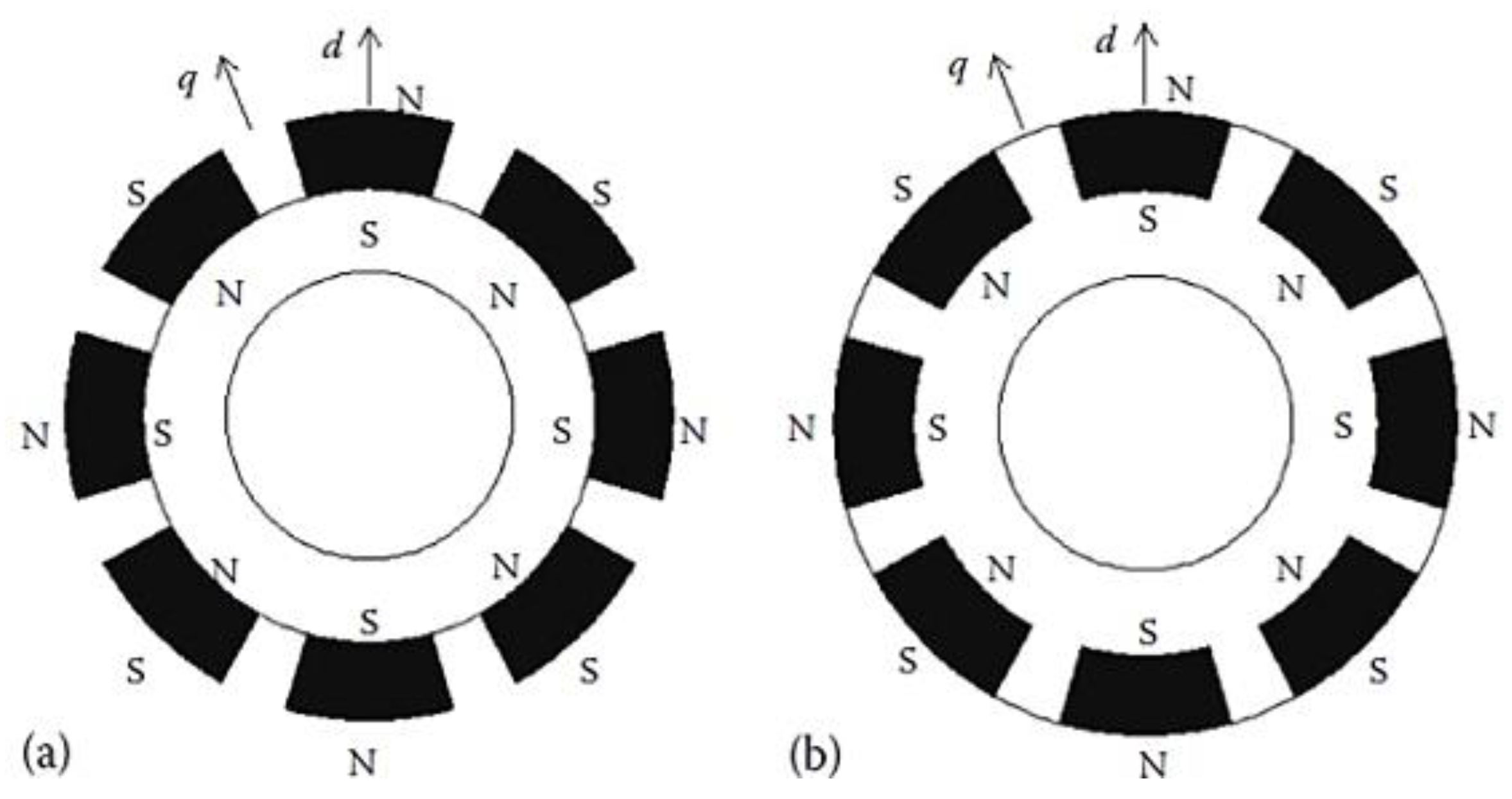
2.1. Model of the PMSM
2.2. Field-Oriented Control Scheme
3. Back-EMF-Based Sensorless Algorithms
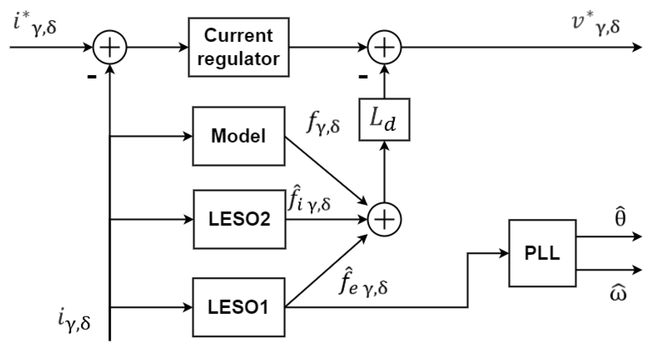
3.1. Sensorless Algorithm Based on Linear Disturbance Observer
- and represent the known model quantities since they are expressed as a function of the motor parameters, currents and speed as in (11)
- and represent the unknown external disturbances as they are expressed as a function of the back-EMFs as in (12)
- and represent the unknown internal disturbances, which are caused by uncertainties in the motor parameters. They are expressed as a function of , , and , which are the variations of the real parameters , , and with respect to their nominal value.
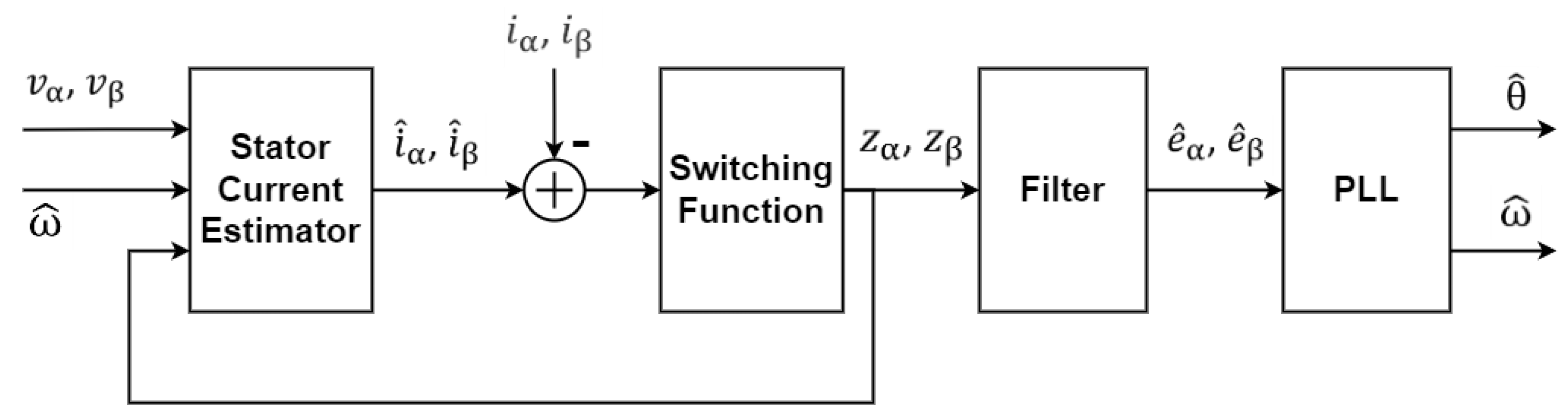
3.2. Sliding Mode Observer
- The selection of the most suitable switching function, which must be chosen among those functions that approximate the behavior of the signum function used in the basic scheme but generate a lower high-frequency content.
- The adoption of the most effective filter, replacing the traditionally used lowpass filter, which introduces a phase shift, resulting in a delay in the estimation process.
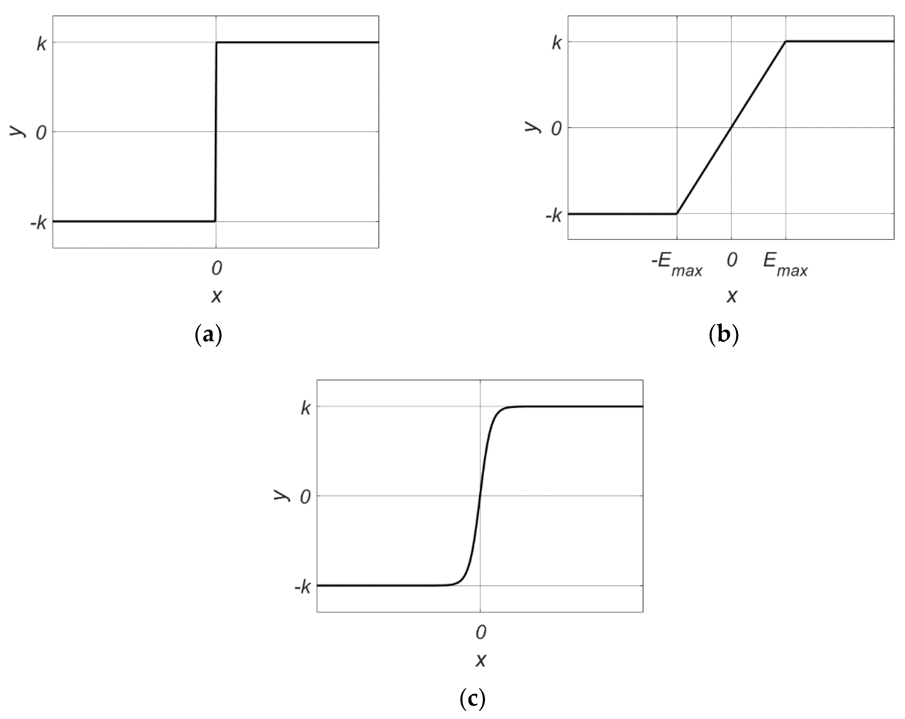
- The traditional signum function (16), shown in Figure 7a, which is the easiest to be implemented but generates the worst signal spectrum in terms of high-frequency content.
- A possible alternative to the previous functions is the super-twisting algorithm [34,35,36]. Unlike the previous ones, it does not consist of a simple function but of a control law obtained by inserting the signum function into an integral filter. The resulting expression for , is given by (21), where , are the two gains
4. Rotor Flux Observer-Based Sensorless Algorithms
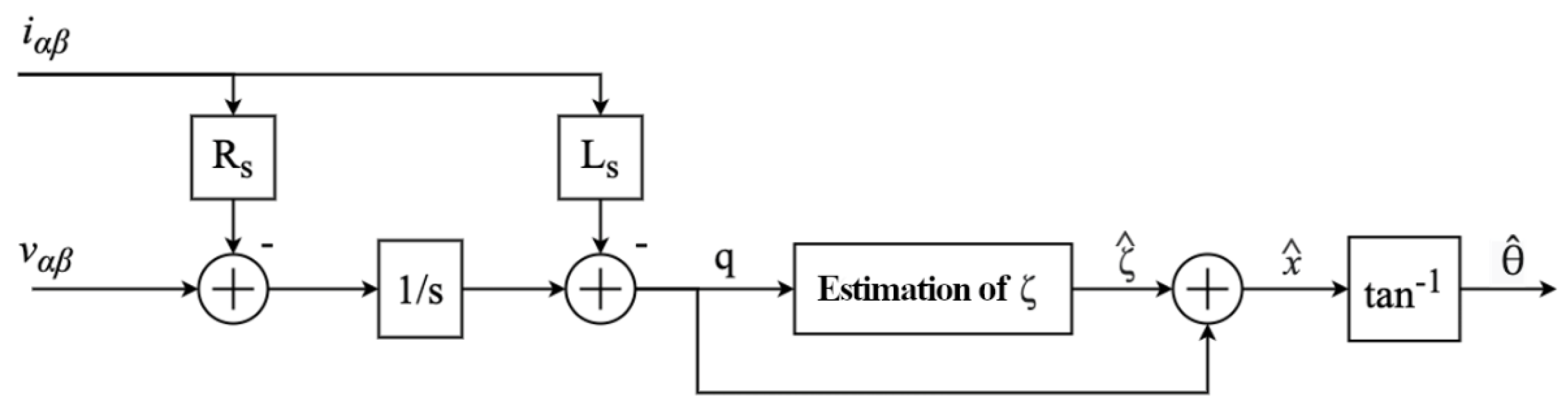
4.1. Nonlinear RFO
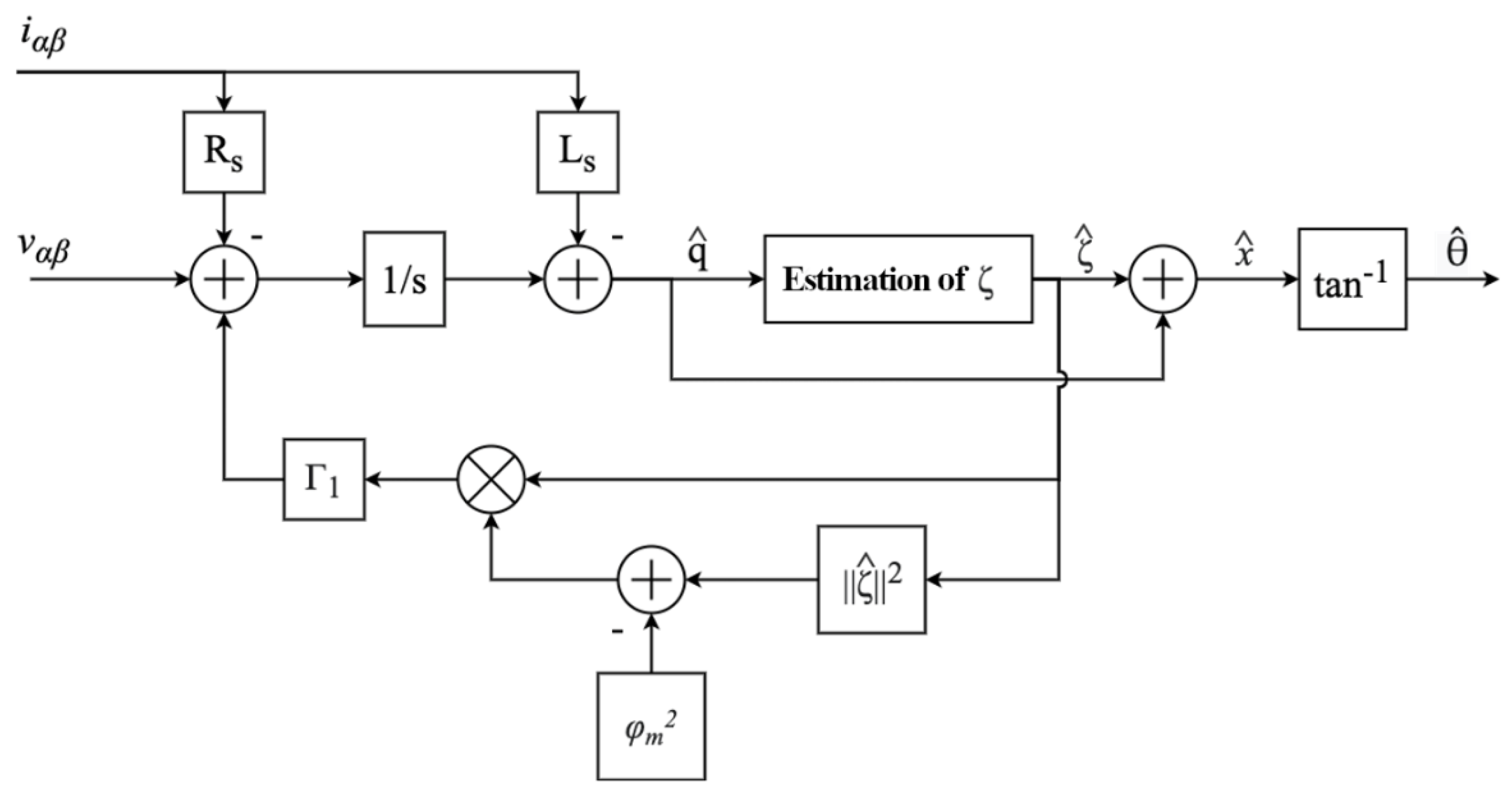
4.2. Adaptive RFO
4.3. Regression RFO
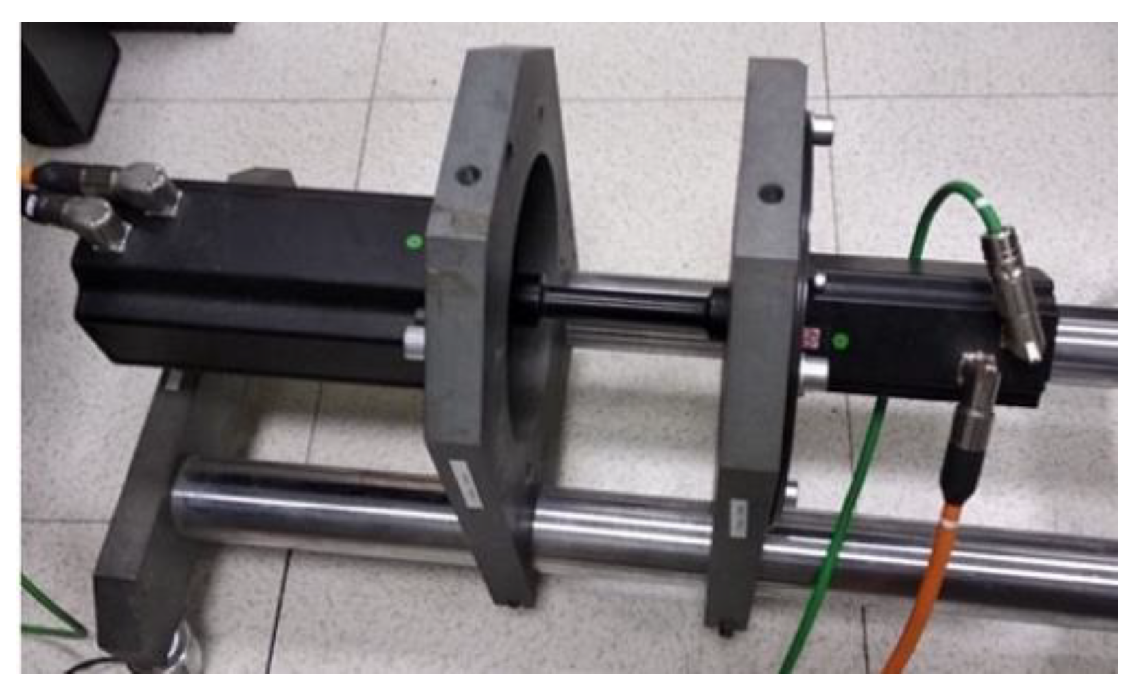
5. Comparison of Different Sensorless Algorithms in the Low-Speed Region on a Test Bench with an SPMSM
- The ease of implementation and computational complexity required for the operation. This can be a critical aspect since some algorithms characterized by a particularly low estimation error may require an intensive computational effort and could increase the overall cost and operating stability of the system. The choice of the most suitable algorithm in this sense should be made taking into account the precision required in estimating the position and the computational resources available.
- The complexity of the tuning process, for what concerns observer gains, cutoff frequency of filters and other parameters. Some applications may expect the algorithm to be used in conditions that are always the same, requiring only one preliminary calibration of the operating parameters. Instead, other applications may require the tuning process to be particularly easy and fast as it may be carried out by the customer depending on the specific purpose.
- The operating speed range. Some applications require the algorithm to be effective in a wide speed range, e.g., from standstill to the nominal speed, while in some other cases the motor is expected to operate at a fixed speed. This aspect can be particularly critical when approaching the low-speed region.
- The type of load. The stability and the dynamic response of a sensorless algorithm often depends on how the load is applied to the motor. For example, some applications such as compressors, ventilation systems or transports usually have a speed-dependent load, while in some cases the system must be able to withstand sudden load steps.
- The robustness against parameter variations. In most cases, the algorithm requires the knowledge of some motor parameters to operate correctly, such as the stator resistance and inductance or the flux linkage constants. These parameters are often not known with sufficient precision and can also change during the operation (e.g., the stator resistance can vary with temperature). For some applications, the system is required to maintain a low estimation error even in the presence of strong variations or mismatches of the motor parameters.
- The “Enhanced Linear Active Disturbance Rejection Controller” (ELADRC), a method based on direct back-EMF estimation by means of LESOs, described in [21].
- A sliding-mode back-EMF observer with the adoption of the frequency adaptive filter, the “FACCF-SMO” described in [33].
- The nonlinear RFO described in [42].
- The adaptive RFO (evolution of the original Bobtsov’s observer) described in [45].
- The regression RFO described in [50].
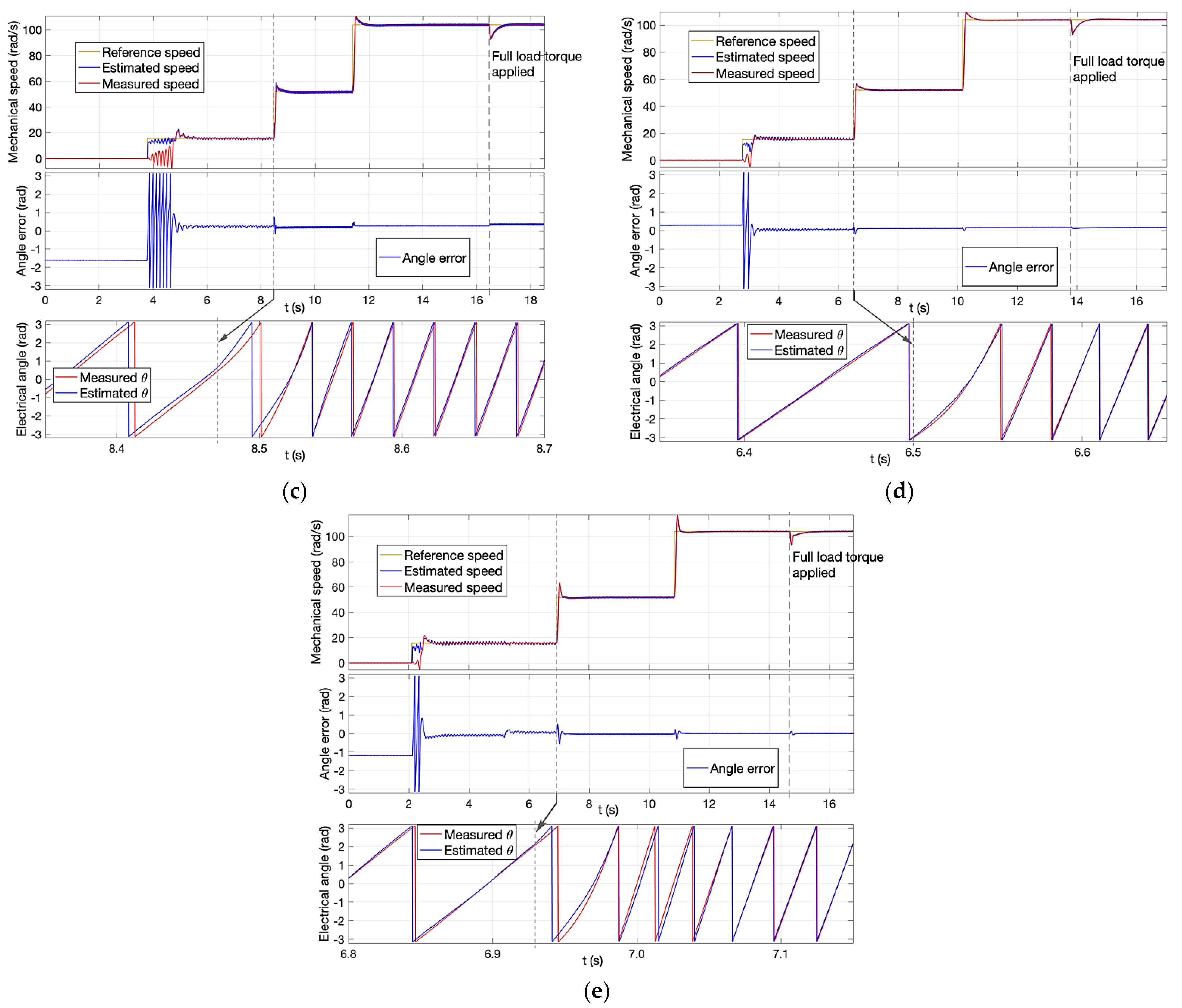
5.1. Performance of the Algorithms during Speed Steps
5.2. Performance of the Algorithms during Load Steps at 10% of Rated Speed
5.3. Performance of the Algorithms during Full Load Starting
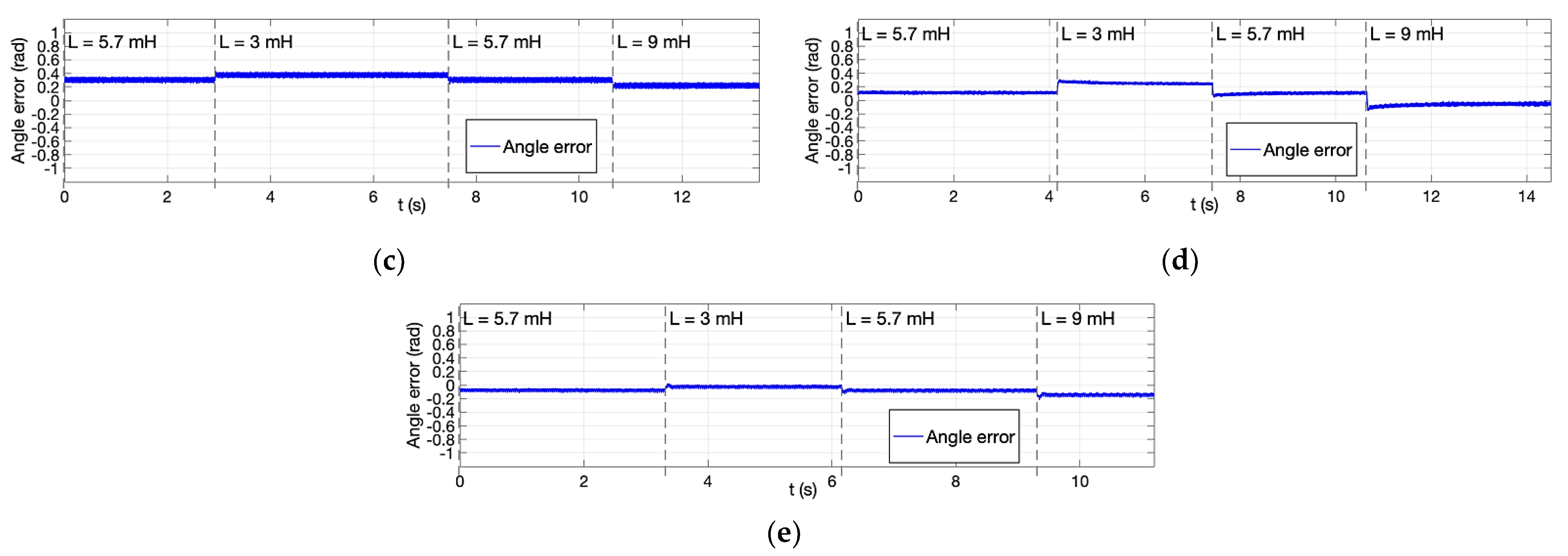
5.4. Robustness of the Algorithms against Inductance Variations
6. Conclusions
Author Contributions
Funding
Conflicts of Interest
References
- Guo, L.; Yang, Z.; Lin, F. A Novel Strategy for Sensorless Control of IPMSM with Error Compensation Based on Rotating High Frequency Carrier Signal Injection. Energies 2020, 13, 1919. [Google Scholar] [CrossRef]
- Kumar, P.; Bottesi, O.; Calligaro, S.; Alberti, L.; Petrella, R. Self-Adaptive High-Frequency Injection Based Sensorless Control for Interior Permanent Magnet Synchronous Motor Drives. Energies 2019, 12, 3645. [Google Scholar] [CrossRef] [Green Version]
- Szalay, I.; Fodor, D.; Enisz, K.; Medve, H. Permanent Magnet Synchronous Motor Model Extension for High-Frequency Signal Injection-Based Sensorless Magnet Polarity Detection. Energies 2022, 15, 1131. [Google Scholar] [CrossRef]
- Yu, K.; Wang, Z.; Li, L. An Optimized Time Sequence for Sensorless Control of IPMSM Drives via High-Frequency Square-Wave Signal Injection Scheme. Energies 2022, 15, 2246. [Google Scholar] [CrossRef]
- Tian, L.; Zhao, J.; Sun, J. Sensorless Control of Interior Permanent Magnet Synchronous Motor in Low-Speed Region Using Novel Adaptive Filter. Energies 2016, 9, 1084. [Google Scholar] [CrossRef] [Green Version]
- Urbanski, K.; Janiszewski, D. Position Estimation at Zero Speed for PMSMs Using Artificial Neural Networks. Energies 2021, 14, 8134. [Google Scholar] [CrossRef]
- Wang, S.; Zhao, J.; Yang, K. High Frequency Square-Wave Voltage Injection Scheme-Based Position Sensorless Control of IPMSM in the Low- and Zero- Speed Range. Energies 2019, 12, 4776. [Google Scholar] [CrossRef] [Green Version]
- Alaei, A.; Nejad, S.M.S.; Gieras, J.F.; Lee, D.; Ahn, J. Reduction of high-frequency injection losses, acoustic noise and total harmonic distortion in IPMSM sensorless drives. IET Power Electron. 2019, 12, 3197–3207. [Google Scholar] [CrossRef]
- Pando-Acedo, J.; Romero-Cadaval, E.; Milanes-Montero, M.I.; Barrero-Gonzalez, F. Improvements on a Sensorless Scheme for a Surface-Mounted Permanent Magnet Synchronous Motor Using Very Low Voltage Injection. Energies 2020, 13, 2732. [Google Scholar] [CrossRef]
- Ha, J.-I.; Ide, K.; Sawa, T.; Sul, S.-K. Sensorless rotor position estimation of an interior permanent-magnet motor from initial states. IEEE Trans. Ind. Appl. 2003, 39, 761–767. [Google Scholar] [CrossRef]
- Jansen, P.; Lorenz, R. Transducerless position and velocity estimation in induction and salient AC machines. IEEE Trans. Ind. Appl. 1995, 31, 240–247. [Google Scholar] [CrossRef] [Green Version]
- Imai, N.; Morimoto, S.; Sanada, M.; Takeda, Y. 3-phase High Frequency Voltage Input Sensorless Control for Hybrid Electric Vehicle Applications. World Electr. Veh. J. 2007, 1, 279–285. [Google Scholar] [CrossRef] [Green Version]
- Jung, T.-U.; Jang, J.-H.; Park, C.-S. A Back-EMF Estimation Error Compensation Method for Accurate Rotor Position Estimation of Surface Mounted Permanent Magnet Synchronous Motors. Energies 2017, 10, 1160. [Google Scholar] [CrossRef] [Green Version]
- Chen, G.-R.; Yang, S.-C.; Hsu, Y.-L.; Li, K. Position and Speed Estimation of Permanent Magnet Machine Sensorless Drive at High Speed Using an Improved Phase-Locked Loop. Energies 2017, 10, 1571. [Google Scholar] [CrossRef] [Green Version]
- You, Z.-C.; Yang, S.-M. A Restarting Strategy for Back-EMF-Based Sensorless Permanent Magnet Synchronous Machine Drive. Energies 2019, 12, 1818. [Google Scholar] [CrossRef] [Green Version]
- Chen, Z.; Tomita, M.; Doki, S.; Okuma, S. An extended electromotive force model for sensorless control of interior permanent-magnet synchronous motors. IEEE Trans. Ind. Electron. 2003, 50, 288–295. [Google Scholar] [CrossRef]
- Wang, G.; Ding, L.; Li, Z.; Xu, J.; Zhang, G.; Zhan, H.; Ni, R.; Xu, D. Enhanced Position Observer Using Second-Order Generalized Integrator for Sensorless Interior Permanent Magnet Synchronous Motor Drives. IEEE Trans. Energy Convers. 2014, 29, 486–495. [Google Scholar] [CrossRef]
- Kim, J.; Jeong, I.; Nam, K.; Yang, J.; Hwang, T. Sensorless Control of PMSM in a High-Speed Region Considering Iron Loss. IEEE Trans. Ind. Electron. 2015, 62, 6151–6159. [Google Scholar] [CrossRef]
- Jiang, F.; Yang, F.; Sun, S.; Yang, K. Static-Errorless Rotor Position Estimation Method Based on Linear Extended State Observer for IPMSM Sensorless Drives. Energies 2022, 15, 1943. [Google Scholar] [CrossRef]
- Du, B.; Wu, S.; Han, S.; Cui, S. Application of Linear Active Disturbance Rejection Controller for Sensorless Control of Internal Permanent-Magnet Synchronous Motor. IEEE Trans. Ind. Electron. 2016, 63, 3019–3027. [Google Scholar] [CrossRef]
- Qu, L.; Qiao, W.; Qu, L. An Enhanced Linear Active Disturbance Rejection Rotor Position Sensorless Control for Permanent Magnet Synchronous Motors. IEEE Trans. Power Electron. 2019, 35, 6175–6184. [Google Scholar] [CrossRef]
- Cho, Y. Improved Sensorless Control of Interior Permanent Magnet Sensorless Motors Using an Active Damping Control Strategy. Energies 2016, 9, 135. [Google Scholar] [CrossRef] [Green Version]
- Moradian, M.; Soltani, J.; Benbouzid, M.; Najjar-Khodabakhsh, A. A Parameter Independent Stator Current Space-Vector Reference Frame-Based Sensorless IPMSM Drive Using Sliding Mode Control. Energies 2021, 14, 2365. [Google Scholar] [CrossRef]
- Hoai, H.-K.; Chen, S.-C.; Than, H. Realization of the Sensorless Permanent Magnet Synchronous Motor Drive Control System with an Intelligent Controller. Electronics 2020, 9, 365. [Google Scholar] [CrossRef] [Green Version]
- Yin, Q.; Li, H.; Luo, H.; Wang, Q.; Xu, C. An Improved Sensorless Vector Control Method for IPMSM Drive with Small DC-Link Capacitors. Energies 2020, 13, 580. [Google Scholar] [CrossRef] [Green Version]
- Chen, J.; Chen, S.; Wu, X.; Tan, G.; Hao, J. A Super-Twisting Sliding-Mode Stator Flux Observer for Sensorless Direct Torque and Flux Control of IPMSM. Energies 2019, 12, 2564. [Google Scholar] [CrossRef] [Green Version]
- Bao, D.; Wu, H.; Wang, R.; Zhao, F.; Pan, X. Full-Order Sliding Mode Observer Based on Synchronous Frequency Tracking Filter for High-Speed Interior PMSM Sensorless Drives. Energies 2020, 13, 6511. [Google Scholar] [CrossRef]
- Wang, Y.; Wang, X.; Xie, W.; Dou, M. Full-Speed Range Encoderless Control for Salient-Pole PMSM with a Novel Full-Order SMO. Energies 2018, 11, 2423. [Google Scholar] [CrossRef] [Green Version]
- Chi, S.; Zhang, Z.; Xu, L. Sliding-Mode Sensorless Control of Direct-Drive PM Synchronous Motors for Washing Machine Applications. IEEE Trans. Ind. Appl. 2009, 45, 582–590. [Google Scholar] [CrossRef]
- Liu, Z.; Chen, W. Research on an Improved Sliding Mode Observer for Speed Estimation in Permanent Magnet Synchronous Motor. Processes 2022, 10, 1182. [Google Scholar] [CrossRef]
- Kim, H.; Son, J.; Lee, J. A High-Speed Sliding-Mode Observer for the Sensorless Speed Control of a PMSM. IEEE Trans. Ind. Electron. 2011, 58, 4069–4077. [Google Scholar] [CrossRef]
- Qiao, Z.; Shi, T.; Wang, Y.; Yan, Y.; Xia, C.; He, X. New Sliding-Mode Observer for Position Sensorless Control of Permanent-Magnet Synchronous Motor. IEEE Trans. Ind. Electron. 2012, 60, 710–719. [Google Scholar] [CrossRef]
- An, Q.; Zhang, J.; An, Q.; Liu, X.; Shamekov, A.; Bi, K. Frequency-Adaptive Complex-Coefficient Filter-Based Enhanced Sliding Mode Observer for Sensorless Control of Permanent Magnet Synchronous Motor Drives. IEEE Trans. Ind. Appl. 2019, 56, 335–343. [Google Scholar] [CrossRef]
- Liang, D.; Li, J.; Qu, R. Sensorless Control of Permanent Magnet Synchronous Machine Based on Second-Order Sliding-Mode Observer with Online Resistance Estimation. IEEE Trans. Ind. Appl. 2017, 53, 3672–3682. [Google Scholar] [CrossRef]
- Liu, Y.; Fang, J.; Tan, K.; Huang, B.; He, W. Sliding Mode Observer with Adaptive Parameter Estimation for Sensorless Control of IPMSM. Energies 2020, 13, 5991. [Google Scholar] [CrossRef]
- Zhao, Y.; Yu, H.; Wang, S. An Improved Super-Twisting High-Order Sliding Mode Observer for Sensorless Control of Permanent Magnet Synchronous Motor. Energies 2021, 14, 6047. [Google Scholar] [CrossRef]
- Kyslan, K.; Petro, V.; Bober, P.; Šlapák, V.; Ďurovský, F.; Dybkowski, M.; Hric, M. A Comparative Study and Optimization of Switching Functions for Sliding-Mode Observer in Sensorless Control of PMSM. Energies 2022, 15, 2689. [Google Scholar] [CrossRef]
- Cui, J.; Xing, W.; Qin, H.; Hua, Y.; Zhang, X.; Liu, X. Research on Permanent Magnet Synchronous Motor Control System Based on Adaptive Kalman Filter. Appl. Sci. 2022, 12, 4944. [Google Scholar] [CrossRef]
- Dilys, J.; Stankevič, V.; Łuksza, K. Implementation of Extended Kalman Filter with Optimized Execution Time for Sensorless Control of a PMSM Using ARM Cortex-M3 Microcontroller. Energies 2021, 14, 3491. [Google Scholar] [CrossRef]
- Shahzad, K.; Jawad, M.; Ali, K.; Akhtar, J.; Khosa, I.; Bajaj, M.; Elattar, E.E.; Kamel, S. A Hybrid Approach for an Efficient Estimation and Control of Permanent Magnet Synchronous Motor with Fast Dynamics and Practically Unavailable Measurements. Appl. Sci. 2022, 12, 4958. [Google Scholar] [CrossRef]
- Urbanski, K.; Janiszewski, D. Sensorless Control of the Permanent Magnet Synchronous Motor. Sensors 2019, 19, 3546. [Google Scholar] [CrossRef] [PubMed] [Green Version]
- Ortega, R.; Praly, L.; Astolfi, A.; Lee, J.; Nam, K. Estimation of Rotor Position and Speed of Permanent Magnet Synchronous Motors With Guaranteed Stability. IEEE Trans. Control Syst. Technol. 2010, 19, 601–614. [Google Scholar] [CrossRef]
- Lee, J.; Hong, J.; Nam, K.; Ortega, R.; Praly, L.; Astolfi, A. Sensorless Control of Surface-Mount Permanent-Magnet Synchronous Motors Based on a Nonlinear Observer. IEEE Trans. Power Electron. 2009, 25, 290–297. [Google Scholar] [CrossRef] [Green Version]
- Bobtsov, A.A.; Pyrkin, A.A.; Ortega, R.; Vukosavic, S.N.; Stankovic, A.M.; Panteley, E.V. A robust globally convergent position observer for the permanent magnet synchronous motor. Automatica 2015, 61, 47–54. [Google Scholar] [CrossRef]
- Choi, J.; Nam, K.; Bobtsov, A.A.; Pyrkin, A.; Ortega, R. Robust Adaptive Sensorless Control for Permanent-Magnet Synchronous Motors. IEEE Trans. Power Electron. 2016, 32, 3989–3997. [Google Scholar] [CrossRef]
- Marchesoni, M.; Passalacqua, M.; Vaccaro, L.; Calvini, M.; Venturini, M. Low Speed Performance Improvement in a Self-Commissioned Sensorless PMSM Drive Based on Rotor Flux Observer. In Proceedings of the 2019 21st European Con-ference on Power Electronics and Applications (EPE ‘19 ECCE Europe), Genova, Italy, 3–5 September 2019; pp. 1–10. [Google Scholar]
- Marchesoni, M.; Passalacqua, M.; Vaccaro, L.; Calvini, M.; Venturini, M. An Improved Low-Noise Sensorless PMSM Drive able to Face Highly Intermittent Load Torque. In Proceedings of the 2019 IEEE 10th International Symposium on Sensorless Control for Electrical Drives (SLED), Turin, Italy, 9–10 September 2019; pp. 1–6. [Google Scholar]
- Marchesoni, M.; Passalacqua, M.; Vaccaro, L.; Calvini, M.; Venturini, M. Performance improvement in a sensorless surface-mounted PMSM drive based on rotor flux observer. Control Eng. Pract. 2019, 96, 104276. [Google Scholar] [CrossRef]
- Carbone, L.; Cosso, S.; Marchesoni, M.; Passalacqua, M.; Vaccaro, L. State-Space Approach for SPMSM Sensorless Passive Algorithm Tuning. Energies 2021, 14, 7180. [Google Scholar] [CrossRef]
- Choi, J.; Nam, K.; Bobtsov, A.A.; Ortega, R. Sensorless Control of IPMSM Based on Regression Model. IEEE Trans. Power Electron. 2018, 34, 9191–9201. [Google Scholar] [CrossRef]
- Choi, J. Regression Model-Based Flux Observer for IPMSM Sensorless Control with Wide Speed Range. Energies 2021, 14, 6249. [Google Scholar] [CrossRef]
- Mubarok, M.S.; Liu, T.-H.; Tsai, C.-Y.; Wei, Z.-Y. A Wide-Adjustable Sensorless IPMSM Speed Drive Based on Current Deviation Detection under Space-Vector Modulation. Energies 2020, 13, 4431. [Google Scholar] [CrossRef]
- Wang, B.; Wang, Y.; Feng, L.; Jiang, S.; Wang, Q.; Hu, J. Permanent-Magnet Synchronous Motor Sensorless Control Using Proportional-Integral Linear Observer with Virtual Variables: A Comparative Study with a Sliding Mode Observer. Energies 2019, 12, 877. [Google Scholar] [CrossRef] [Green Version]
- Benevieri, A.; Marchesoni, M.; Passalacqua, M.; Vaccaro, L. Experimental Low-Speed Performance Evaluation and Comparison of Sensorless Passive Algorithms for SPMSM. IEEE Trans. Energy Convers. 2021, 37, 654–664. [Google Scholar] [CrossRef]


| Parameter | Value |
|---|---|
| Rated output power | 1000 W |
| Number of poles | 8 |
| Rated speed | 520 rad/s |
| Rated voltage | 376 V |
| Maximum current | 2.21 A |
| Rated torque | 2 Nm |
| Stator resistance Rs | 1.6 Ω |
| Stator inductance Ls | 5.7 mH |
| Flux constant φm | 0.147 Wb |
| Algorithm | Angle Estimation Error (rad) Mean Value/Ripple Amplitude | Starting Time 0–3% ωN | |||
|---|---|---|---|---|---|
| 3% ωN | 10% ωN | 20% ωN | Full Load Applied | ||
| ELADRC | 0.15/0.4 | 0.28/0.03 | 0.45/0.02 | Not successful | 0.2 s |
| FACCF-SMO | 0.15/0.3 | 0.2/0.3 | 0.3/0.25 | Not successful | 0.3 s |
| Nonlinear RFO | 0.25/0.18 | 0.2/0.09 | 0.27/0.07 | 0.36/0.08 | 1.1 s |
| Adaptive RFO | 0.05/0.14 | 0.12/0.04 | 0.18/0.04 | 0.16/0.05 | 0.4 s |
| Regression RFO | −0.1/0.12 | −0.03/0.05 | 0.0/0.04 | 0.01/0.05 | 0.4 s |
| Algorithm | Angle Estimation Error (rad) Mean Value/Variation from the No-Load Condition | |
|---|---|---|
| Half Load Applied | Full Load Applied | |
| ELADRC | 0.33/Δεθ = 0.05 | 0.39/Δεθ = 0.11 |
| FACCF-SMO | 0.25/Δεθ = 0.05 | Not successful |
| Nonlinear RFO | 0.25/Δεθ = 0.05 | 0.3/Δεθ = 0.1 |
| Adaptive RFO | N.A. | 0.12/Δεθ = 0 |
| Regression RFO | N.A. | −0.08/Δεθ = −0.05 |
| Algorithm | Angle Estimation Error (rad) Mean Value/Variation from the Real Inductance Condition | |
|---|---|---|
| Ls = 3 mH | Ls = 9 mH | |
| ELADRC | 0.48/Δεθ = 0.09 | 0.31/Δεθ = −0.08 |
| FACCF-SMO | 0.3/Δεθ = 0.05 | Unstable |
| Nonlinear RFO | 0.38/Δεθ = 0.08 | 0.22/Δεθ = −0.08 |
| Adaptive RFO | 0.25/Δεθ = 0.13 | −0.05/Δεθ = −0.17 |
| Regression RFO | −0.03/Δεθ = 0.05 | −0.15/Δεθ = −0.07 |
Publisher’s Note: MDPI stays neutral with regard to jurisdictional claims in published maps and institutional affiliations. |
© 2022 by the authors. Licensee MDPI, Basel, Switzerland. This article is an open access article distributed under the terms and conditions of the Creative Commons Attribution (CC BY) license (https://creativecommons.org/licenses/by/4.0/).
Share and Cite
Benevieri, A.; Carbone, L.; Cosso, S.; Kumar, K.; Marchesoni, M.; Passalacqua, M.; Vaccaro, L. Surface Permanent Magnet Synchronous Motors’ Passive Sensorless Control: A Review. Energies 2022, 15, 7747. https://doi.org/10.3390/en15207747
Benevieri A, Carbone L, Cosso S, Kumar K, Marchesoni M, Passalacqua M, Vaccaro L. Surface Permanent Magnet Synchronous Motors’ Passive Sensorless Control: A Review. Energies. 2022; 15(20):7747. https://doi.org/10.3390/en15207747
Chicago/Turabian StyleBenevieri, Alessandro, Lorenzo Carbone, Simone Cosso, Krishneel Kumar, Mario Marchesoni, Massimiliano Passalacqua, and Luis Vaccaro. 2022. "Surface Permanent Magnet Synchronous Motors’ Passive Sensorless Control: A Review" Energies 15, no. 20: 7747. https://doi.org/10.3390/en15207747