Article

Model NOx, SO2 Emissions Concentration and Thermal Efficiency of CFBB Based on a Hyper-Parameter Self-Optimized Broad Learning System

1
School of Information Engineering, Tianjin University of Commerce, Beichen, Tianjin 300134, China
2
School of Economics, Tianjin University of Commerce, Beichen, Tianjin 300134, China
3
School of Artificial Intelligence, Hebei University of Technology, Hongqiao, Tianjin 300132, China
*
Author to whom correspondence should be addressed.
Energies 2022, 15(20), 7700; https://doi.org/10.3390/en15207700
Submission received: 14 September 2022 / Revised: 9 October 2022 / Accepted: 14 October 2022 / Published: 18 October 2022

Abstract

:
At present, establishing a multidimensional characteristic model of a boiler combustion system plays an important role in realizing its dynamic optimization and real-time control, so as to achieve the purpose of reducing environmental pollution and saving coal resources. However, the complexity of the boiler combustion process makes it difficult to model it using traditional mathematical methods. In this paper, a kind of hyper-parameter self-optimized broad learning system by a sparrow search algorithm is proposed to model the NOx, SO2 emissions concentration and thermal efficiency of a circulation fluidized bed boiler (CFBB). A broad learning system (BLS) is a novel neural network algorithm, which shows good performance in multidimensional feature learning. However, the BLS has several hyper-parameters to be set in a wide range, so that the optimal combination between hyper-parameters is difficult to determine. This paper uses a sparrow search algorithm (SSA) to select the optimal hyper-parameters combination of the broad learning system, namely as SSA-BLS. To verify the effectiveness of SSA-BLS, ten benchmark regression datasets are applied. Experimental results show that SSA-BLS obtains good regression accuracy and model stability. Additionally, the proposed SSA-BLS is applied to model the combustion process parameters of a 330 MW circulating fluidized bed boiler. Experimental results reveal that SSA-BLS can establish the accurate prediction models for thermal efficiency, NOx emission concentration and SO2 emission concentration, separately. Altogether, SSA-BLS is an effective modelling method.

Graphical Abstract

1. Introduction

Nowadays, the heat and electricity we use are mainly generated through power plants. During the combustion process of a station boiler, large amounts of polluting gases are produced, such as NOx, SO2 and CO2, that cause great harm to the human living environment. Simultaneously, a large amount of coal is consumed. Coal resources are becoming increasingly scarce; the goals of saving energy and emission reduction are imminent. The realization of dynamic multi-objective optimal control of boiler combustion process under variable loads is an effective method to reduce environmental pollution and save coal resources, and is called the boiler combustion optimization problem [1,2]. In order to solve the problem, the first priority is to establish the multi-dimensional feature model of the boiler combustion system. However, the boiler combustion system has complex characteristics with nonlinearity, strong coupling and large hysteresis, making it difficult to be modeled by traditional mathematical mechanistic methods. Zhou et al. have successively applied artificial neural networks or support vector machines (SVM) [3,4] combined with swarm intelligence optimization algorithms to model boiler combustion systems [5,6,7,8,9,10]. For example, ref. [5] combined ANN with genetic algorithms (GA), ref. [7] combined SVM and a meta-genetic algorithm (MGA), and ref. [9] combined SVM and ant colony optimization (ACO) [11]. These research results showed that good prediction results could be obtained via applying artificial neural networks and support vector machines. Li and Ma et al. applied various improved extreme learning machine (ELM) models [12,13,14] to establish prediction models for boiler thermal efficiency, NOx emission concentration or SO2 emission concentration [15,16,17,18,19,20,21]. For example, Li et al. proposed the fast-learning networks (FNN) by connecting the input and output layers of ELM and implemented the fast modeling of boiler combustion systems; Ma et al. proposed an improved online sequential ELM and implemented the real-time modeling of boiler combustion systems. However, it was proven that in traditional ANN and ELM there exists an over-fitting problem when solving small sample data regression problems. In addition, the model computation speed of SVM is slow when solving the large sample data regression problem. This paper firstly uses a newly neural network, called broad learning system [22], to solve the modeling problem of boiler combustion systems.
Broad learning system (BLS), as a new neural network algorithm proposed in 2018, has greater advantages in multi-dimensional feature learning and computing time compared to other deep learning algorithms, such as deep belief network (DBN) [23], deep boltzmann machine (DBM) [24] and convolutional neural network (CNN) [25]. Chen et al. [26] proposed several variants of BLS to solve regression problems, and experimental results showed that BLS variants had better performance than other state-of-the-art methods, such as conventional BLS, ELM and SVM. BLS has been researched and applied in many fields in recent years [27,28,29,30,31,32,33,34]. For example, Shuang and Chen [33] combined fuzzy system with BLS, proposed a new neuro-fuzzy algorithm, and applied it to solve regression and classification problems. Zhao et al. [34] extended BLS using a stream regularization framework and proposed a new algorithm for semi-supervised learning to solve complex data classification problems. However, the hyper-parameters of BLS could seriously affect its model performance. If the hyper-parameters are set too large, BLS encounters an over-fitting problem and spends more computation time. If the hyper-parameters are set too small, the generalization ability of BLS is weakened. BLS has more hyper-parameters, and every hyper-parameter needs to be set in a wide range, so the optimal combination of several hyper-parameters is difficult to determine by using traditional methods. It is of great research value to design a method to optimize the hyper-parameters of BLS to ensure its good model performance. Nacef et al. [35] leverages deep learning and network optimization techniques to solve various network configuration and scheduling problems, enabling fast self-optimization and the lifecycle management of networks, and demonstrating the great role of optimization techniques in saving runtime and reducing computational costs. In addition, swarm intelligence optimization algorithms can provide substantial benefits in reducing computational effort and improving system performance without a priori knowledge of the system parameters [36]. To address the above-mentioned problem, this paper proposes a kind of hyper-parameter self-optimized broad learning system, namely SSA-BLS. The proposed method mainly introduces the optimization mechanism of sparrow search algorithm [37] to determine the optimal hyper-parameter combination of BLS through three different behaviors of the sparrow population during foraging, i.e., sparrows as explorers provide search directions and regions for the optimal hyper-parameter combinations, sparrows as followers search through the guidance of explorers, and sparrows as vigilantes rely on anti-predation strategy to avoid hyper-parameter combinations from falling into local optima. The sparrow search algorithm (SSA) is a new swarm intelligence optimization algorithm proposed in 2020. Compared with particle swarm optimization (PSO) [38,39], gravitational search algorithm (GSA) [40] and grey wolf optimization (GWO) [41], the SSA had better computation efficiency. This paper combines SSA with BLS to automatically adjust the hyper-parameters and obtain the optimal hyper-parameter combination. In SSA-BLS, a mechanism to achieve automatic optimization of hyperparameters with the objective of minimizing the average root-mean-square-error (RMSE) of the testing set after ten-fold cross-validation [42] is proposed in order to obtain better model accuracy and model stability.
In order to verify the effectiveness of SSA-BLS, it was applied to ten benchmark regression datasets. Compared with BLS, RELM [43] and KELM [44,45], SSA-BLS can achieve the best model accuracy and model stability whose hyper-parameters are determined by using the nested cross-validation method [46].
Simultaneously, the proposed SSA-BLS was applied to establish the prediction comprehensive model of thermal efficiency, NOx emission concentration and SO2 emission concentration. Compared with conventional BLS, the proposed SSA-BLS has better model accuracy and stronger stability. The experimental results reveal that the model accuracy can reach 10−2-10−3 by SSA-BLS.
The contributions of this paper are summarized as follows:
(1)
A novel optimized BLS is proposed. SSA is firstly used to optimize the hyper-parameters of BLS, which can determine the optimal hyper-parameter combination.
(2)
The proposed SSA-BLS is used to solve the regression problem of ten benchmark datasets.
(3)
The proposed SSA-BLS and traditional BLS are firstly applied to establish the prediction conventional model of one circulation fluidized bed boiler combustion system.
The structure of this paper is as follows: basic knowledge and related works are given in Section 2; the proposed SSA-BLS is given in Section 3; Section 4 shows the performance evaluation of the SSA-BLS; Section 5 addresses the real-world modelling problem; the conclusion of this paper is in Section 6.

2. Basic Knowledge and Related Works

2.1. Broad Learning System

Broad learning system (BLS), as a novel artificial neural network algorithm, is capable of replacing deep architecture. It adds a dynamic stepwise update mechanism and a sparse self-coding algorithm to the random vector functional-link neural network (RVFLNN) [47,48,49], which greatly improves the model computing efficiency.
As opposed to RVFLN, BLS replaces the input layer with the mapping layer. The mapping layer of BLS is obtained by sparse representation and linear transformation of the input layer data. The augmentation layer is obtained by applying a nonlinear transformation to the activation function mapping layer. BLS connects the mapping layer and the enhancement layer together with the output layer to solve the connection weight of the neural networks. The structure diagram of BLS is shown in Figure 1.
Where X R N × M is the input data with sample size N and dimension M , and Y R N × 1 is the output data with sample size N and dimension 1.
Assuming that the network structure has n feature mappings and each feature mapping has k feature nodes, the expression of the i th feature mapping Z i is shown in Equation (1).
Z i = ϕ i x 1 W i 1 + β i 1 ϕ i x N W i 1 + β i 1 ϕ i x 1 W i k + β i k ϕ i x N W i k + β i k = ϕ i X W e i + β c i , i = 1 , 2 , , n
where ϕ i denotes the feature mapping function, W i k R M × K is the connection weight of the i th group of feature mappings to all input data and β c i R 1 × K is the bias of the i th group of feature mappings, then the expression of all feature mappings Z n in the feature node layer is shown in Equation (2).
Z n = ϕ 1 X W e 1 + β e 1 ϕ 2 X W e 2 + β e 2 ϕ n X W e n + β e n T = Z 1 Z 2 Z n , j = 1 , 2 , , m
Similarly, the expression for the j th group of enhanced nodes H j is shown in Equation (3).
H j = ζ j Z 1 W j 1 + β j 1 ζ j Z n W j 1 + β j 1 ζ j Z 1 W j l + β j l ζ j Z n W j l + β j l = ζ j Z n W h j + β h j , j = 1 , 2 , , m
where ζ j denotes the activation function, l is the number of the j th group of augmented nodes and W h j R k n × l and β h j R 1 × l are the connection weights and biases randomly generated by the system, then the expression of all the feature augmentation H m in the augmented node layer is shown in Equation (4).
H m = ζ 1 Z n W h 1 + β h 1 ζ 2 Z n W h 2 + β h 2 ζ m Z n W h m + β h m T = H 1 H 2 H m
Then the expression of the final network output Y ^ is shown in Equation (5).
Y ^ = Z 1 , , Z n ζ Z n W h 1 + β h 1 , , ζ Z n W h m + β h m W m       = Z 1 , , Z n H 1 , , H m W m       = Z n H m W m
Then the expression for the final connection weight W m is shown in Equation (6).
W m = Z n H m + Y

2.2. Sparrow Search Algorithm

Sparrow search algorithm (SSA) [34] is a novel swarm intelligence optimization algorithm based on the foraging and anti-predatory behaviors of sparrows. Its bionic principle is as follows: sparrows as explorers provide the search direction and region for the population, sparrows as followers search through the guidance of explorers, and sparrows as vigilantes rely on anti-predation strategies to avoid the population from falling into a local optimal solution.
The location update rules for the three types of sparrows are as follows:
(1)
For sparrows as explorers, when the warning value is less than the safety value, it indicates that the sparrow has not found a predator and can perform a wide range of jumping searches, and when its warning value is greater than or equal to the safety value, it indicates that the sparrow has found a predator and immediately moves to other places for searching.
(2)
For the sparrow as a follower, when its fitness value is less than or equal to half of the sparrows, it indicates that the sparrow did not obtain food and needs to move to other places to search, and when its fitness value is greater than half of the sparrows, it indicates that the sparrow can obtain food and will conduct a random search at the current location.
(3)
For the sparrow as vigilant, when its fitness value is not equal to the current best fitness value, it indicates that the sparrow is at the edge of the population and is highly vulnerable to predators, and when its fitness value is equal to the current best fitness value, it indicates that the sparrow is in the middle of the population and needs to move closer to other sparrows to reduce the risk of being predated.
Suppose there are S sparrows in a D -dimensional search space, then the position of the i th sparrow in the D -dimensional search space is X i = x i a , , x i d , , x i D , i = 1 , 2 , , S , where x i d is the position of the i th sparrow in the d -dimension.
Sparrows as explorers generally account for 10–20% of the population, and their position is updated by the expression shown in Equation (7).
x i d i + 1 = x i d t e x p i α T         R 2 < S T x i d t + Q L         R 2 S T
where t is the current number of iterations; T is the maximum number of iterations; α is a uniform random number between 0 ,   1 ; Q is a random number obeying the standard normal distribution; L is a matrix of size 1 × d and all elements are 1; R 2   0 ,   1 is the warning value; S T   0.5 ,   1 is the safety value.
The other sparrows in the population act as followers, and the expression for their position update is shown in Equation (8).
x i d t + 1 = Q e x p x w d t x i d t i 2         i > n 2 x b d t + 1 + x i d t x b d t + 1 A + L         i n 2
where A is a 1 × D -dimensional matrix; x w d t is the worst position of the sparrow in the d th dimension when the population undergoes the t th iteration; x b d t + 1 is the optimal position of the sparrow in the d th dimension when the population undergoes the t + 1 th iteration.
The sparrows as vigilantes are some sparrows randomly selected from explorers and followers, generally accounting for 10–20% of the population size, and their position update expressions are shown in Equation (9).
x i d t + 1 = x b d t + β x i d t x b d t     f i f g x i d t + K x i d t x w d t f i f w + e         f i = f g
where β and K are step control parameters, β is a random number obeying standard normal distribution, and K is a random number between [ 1 ,     1 ] ; e is a very small constant to avoid the case that the denominator is 0; f i is the fitness value of the ith sparrow; f g and f w are the best fitness value and the worst fitness value in the current sparrow population.

3. The Proposed SSA-BLS

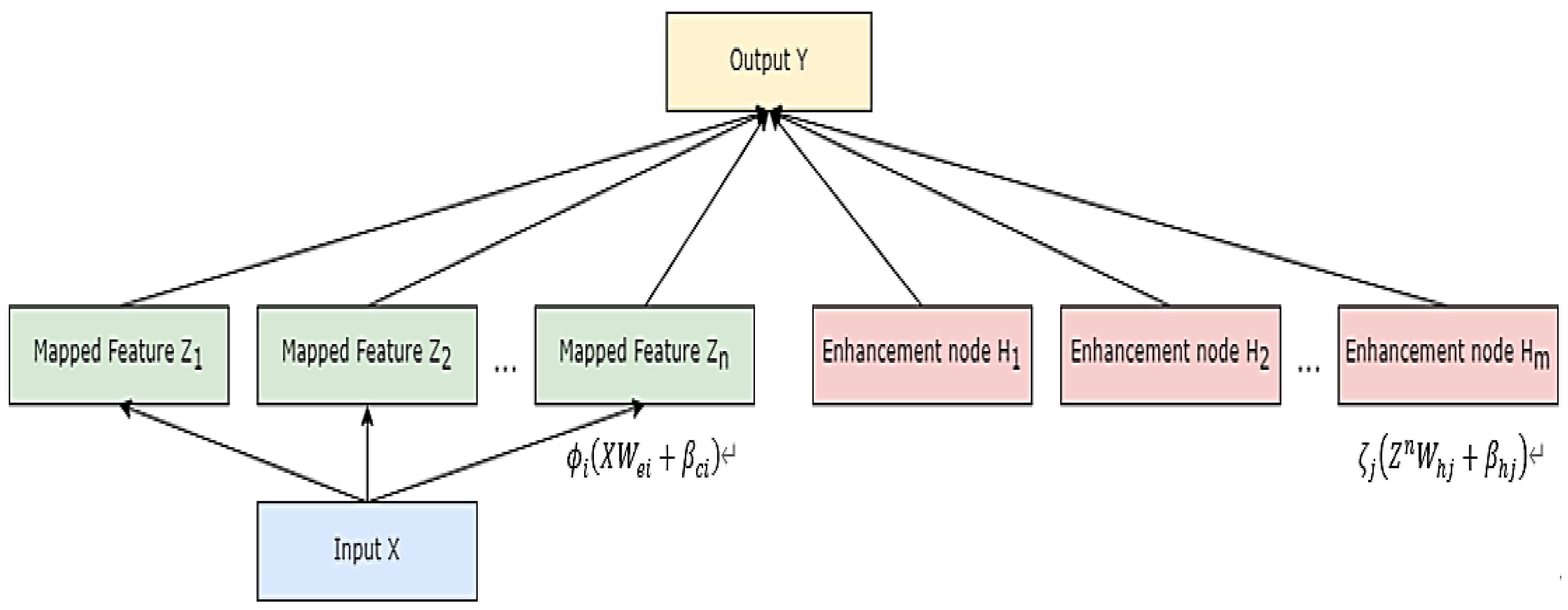
In the BLS model, the randomly generated weights and biases as well as its five hyper-parameters (convergence coefficient s , regularization coefficient c , the number of feature nodes N f , the number of feature mapping groups N m and the number of enhancement nodes N e ) all have an impact on its performance. Among them, the most influential on its model accuracy and model stability are the hyper-parameters N f , N m and N e . However, these three hyper-parameters have a wide range of values, so it is difficult to determine the best combination of hyper-parameters by traditional methods. An optimized broad learning system by sparrow search algorithm with self-adjusting hyper-parameters, i.e., SSA-BLS, is proposed in this paper to enhance the model performance and generalization capability.
The pseudo-code of the proposed SSA-BLS algorithm is shown in Algorithm 1.
Algorithm 1. The pseudo-code of SSA-BLS
Input:
MaxIter: the maximum iterations
dim: the number of hyper-parameters to be optimized
pop: the number of hyper-parameter combination populations
lb&ub: hyper-parameter combination search range
X: the initial population of hyper-parameter combinations
Output:
the optimal hyper-parameter combination X b e s t
best fitness value f b e s t
Iterative Curve I C
1Establish an objective function f x , i.e., the AVG of RMSE
obtained by 10-fold cross-validation;
2Generate pop hyper-parameter combinations as initial population;
3Calculate the fitness values by BLS;
4while t < M a x I t e r   do
5 Randomly select hyper-parameter combinations as explorers,
followers and vigilantes;
6 for each i = e x p l o r e r   do
7 Using Equation (7) to update locations;
8 end
9 for each i = f o l l o w e r   do
10 Using Equation (8) to update locations;
11 end
12 for each i = v i g i l a n t e   do
13 Using Equation (9) to update locations;
14 end
15 Calculate the fitness values by BLS;
16 Compare with previous f b e s t ;
17 ifthe current values better than  f b e s t then
18 Update the f b e s t   and X b e s t ;
19 end
20 Save current f b e s t to I C ;
21 t = t + 1
22end
The determination steps of three hyper-parameters are summarized as follows:
(1)
Generate a certain number of hyper-parameter combinations randomly as the initial population for optimization.
(2)
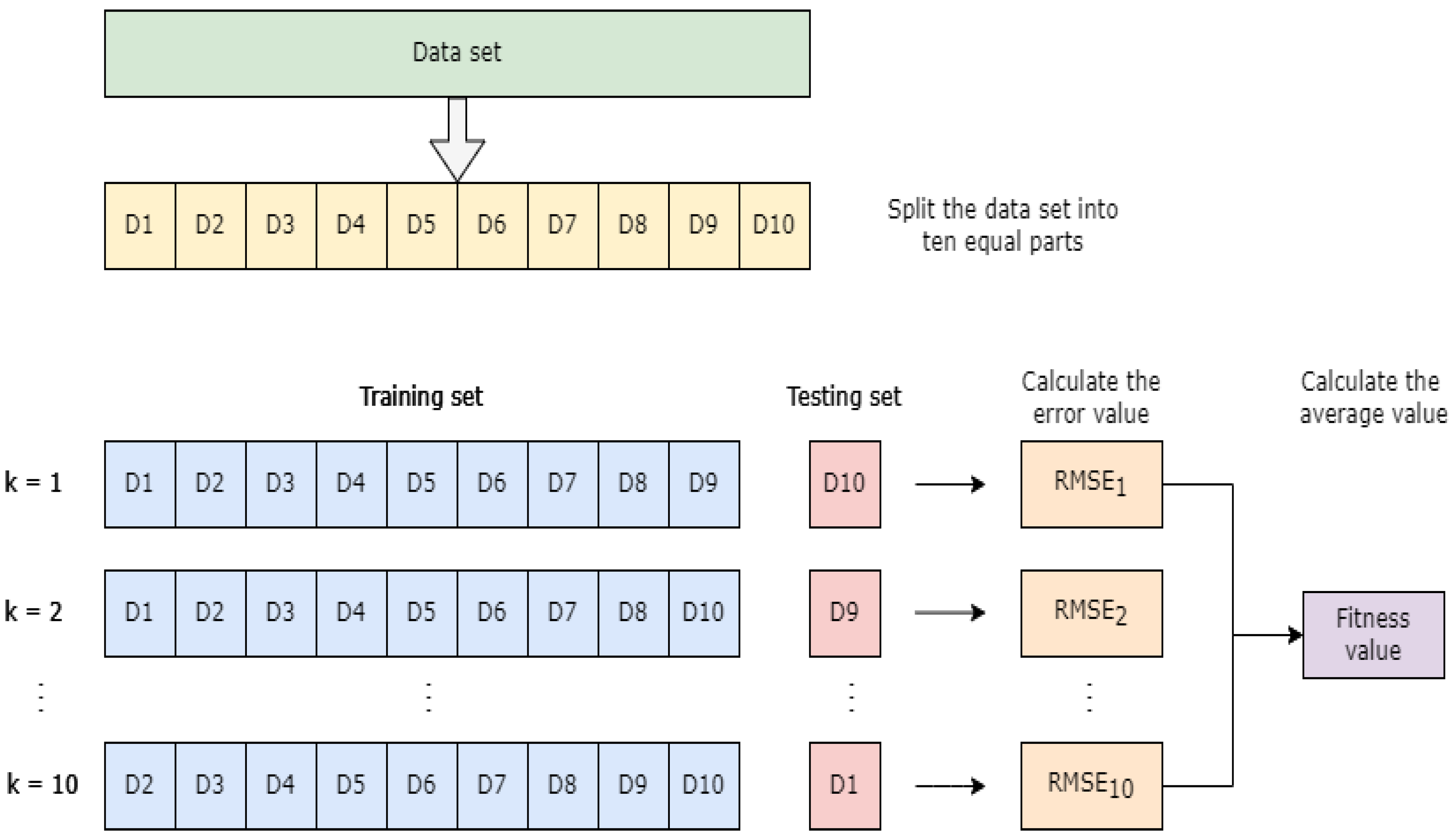
Calculate the fitness value of the hyper-parameter combinations in the initial population, which is the average of the root mean square error (RMSE) obtained by 10-fold cross-validation of the testing set.
The expression for calculating the root mean square error (RMSE) is shown in Equation (10).
R M S E = 1 N i = 1 T y i ^ y i 2
where T is the number of samples, y i denotes the actual value and y i ^ denotes the predicted value.
The schematic diagram of the fitness value calculating process is shown in Figure 2.
(3)
A certain number of hyper-parameter combinations are randomly selected from the initial population as optimized explorers, and the positions are updated according to Equation (7).
(4)
The other hyper-parameter combinations in the initial population act as optimized followers, and the positions are updated according to Equation (8).
(5)
A certain number of hyper-parameter combinations are randomly selected from the optimized explorers and followers as the optimized vigilantes, and the positions are updated according to Equation (9).
(6)
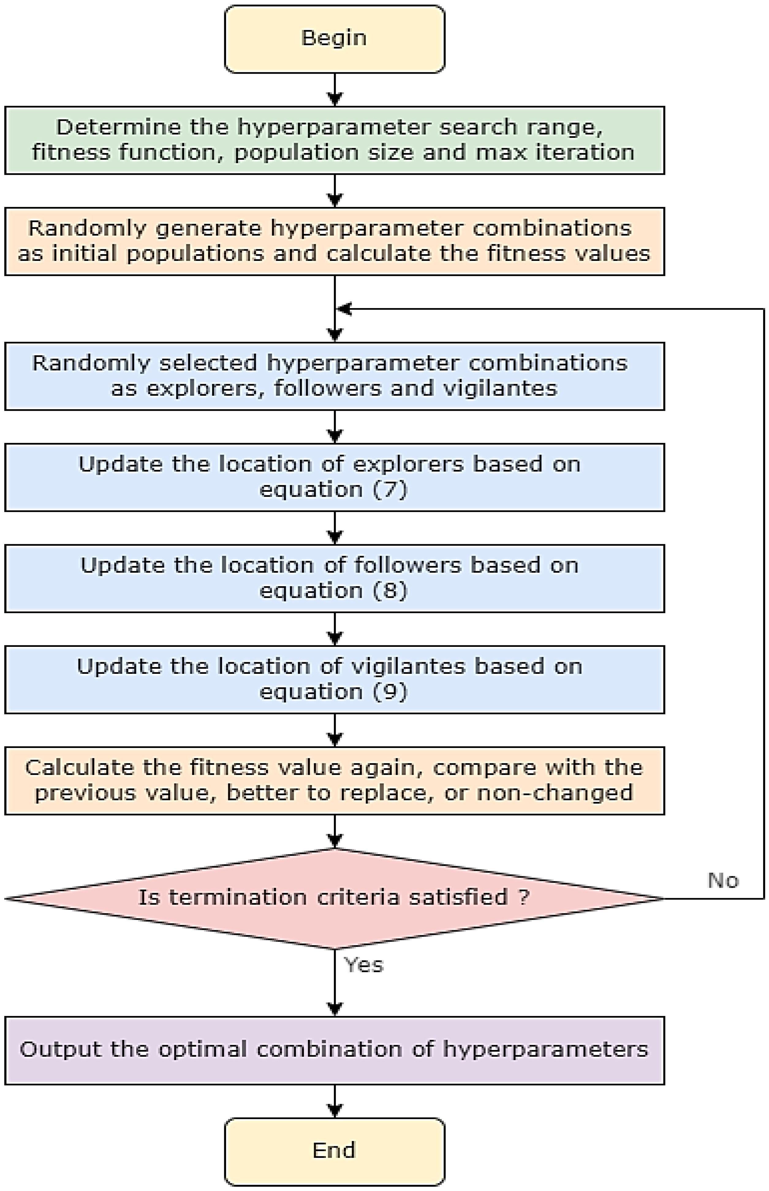
Repeat steps (3)–(5) until the maximum number of iterations is reached, and output the individual with the highest fitness value, i.e., the hyper-parameter combination that makes the smallest average of RMSE obtained from a 10-fold cross-validation of the testing set.
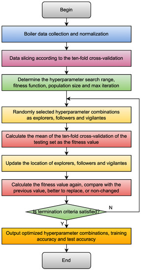
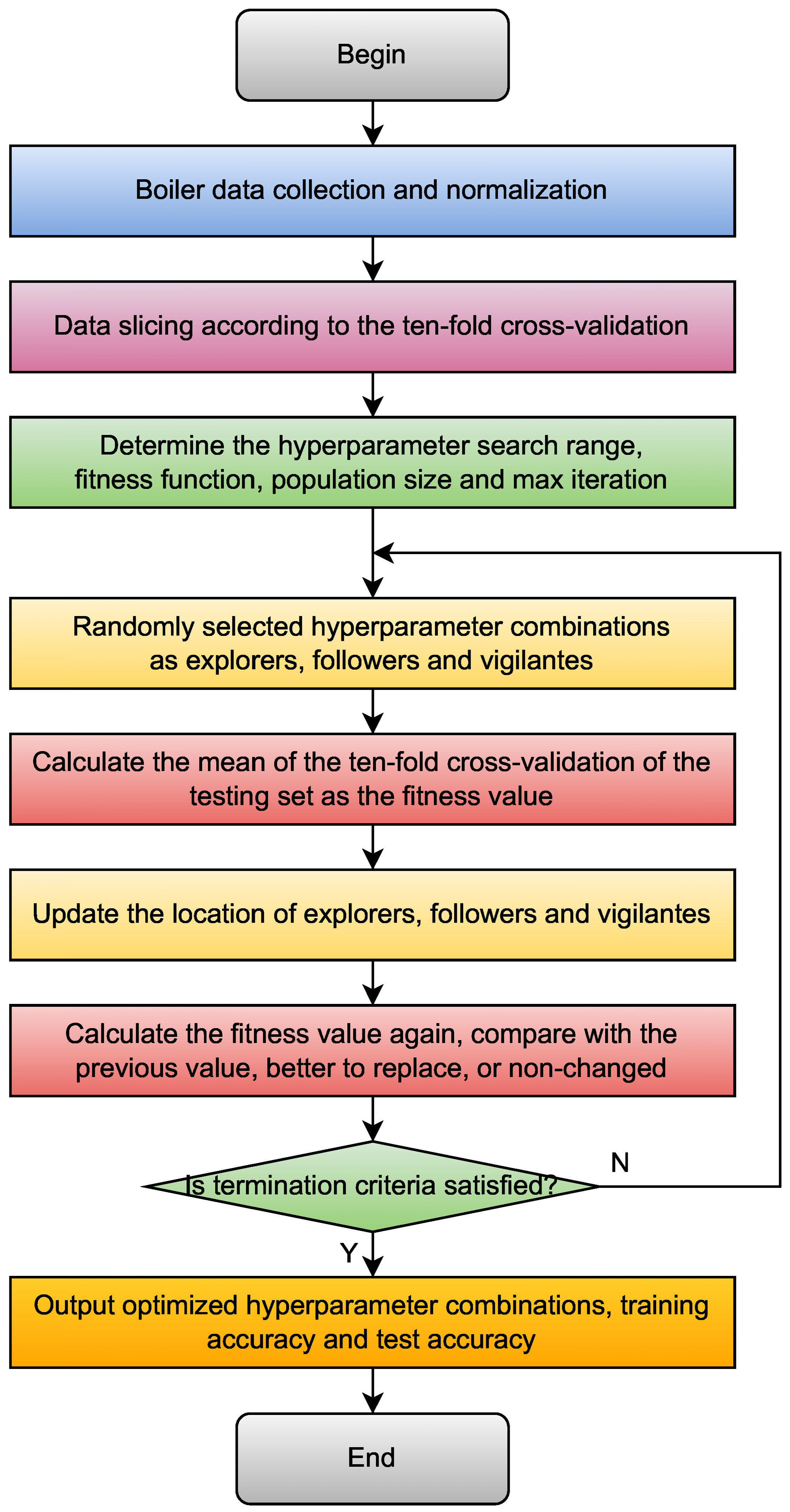
According to the above explanations, the flowchart of the SSA-BLS is shown in Figure 3.

4. Simulation

In order to evaluate the performance of the proposed SSA-BLS, it was applied to the ten benchmark regression datasets listed in Table 1, where the dataset Gasoline octane is from the web: https://www.heywhale.com/home (accessed on 5 January 2022), Fuel consumption is from the web: https://www.datafountain.cn (accessed on 10 January 2022) and the other datasets are from the web: http://www.liaad.up.pt/~ltorgo/Regression/DtaSets.html (accessed on 9 December 2021). All evaluations for RELM, KELM, BLS and SA-ELM were carried out in MacOS Mojave 10.14.6 and Python 3.9.9, running on a laptop with AMD Intel Iris Plus Graphics 645 1536MB, Processor 1.4GHz Intel Core i5 and RAM 8GB 2133MHz.
The parameters in SSA-BLS were set as follows: the initial population size and the maximum number of iterations for hyper-parameter optimization were set to 20 and 100. The compression factor in the mapping layer was set to 0.8 and the regularization factor in the enhancement layer was set to 2. The optimization range of hyper-parameter combination is shown in Table 2.
Model accuracy and model stability were assessed by the average (AVG) and standard deviation (Sd) of the RMSE obtained from the ten-fold cross-validation. The averages (AVG) of the MAPE obtained from the ten-fold cross-validation were also used to evaluate the model accuracy. A smaller average value indicates higher model accuracy, and a smaller standard deviation indicates better model stability, and vice versa.
SSA-BLS was applied to the ten benchmark regression datasets in Table 1 and compared with BLS, RELM and KELM; the simulation results are shown in Table 3, Table 4 and Table 5. The hyper-parameters of the compared algorithm are determined by using the nested cross-validation method [42]. And the bolds in the table indicate the best experimental results of the four algorithms on each dataset.
As shown in Table 4, for the testing samples of the datasets, compared with RELM, KELM and BLS, the proposed SSA-BLS obtains better model accuracy on nine benchmark regression problems (gasoline octane, fuel consumption, abalone, bank domains, Boston housing, delta elevators, forest fires, machine CPU, servo) and better model stability on seven benchmark regression problems (bank domains, Boston housing, forest fires, machine CPU, servo).
As shown in Table 5, for the training samples of the datasets, compared with RELM, KELM and BLS, the proposed SSA-BLS obtains better model performance on all ten benchmark regression problems and for the testing samples of the datasets, the proposed SSA-BLS obtains better model performance on nine benchmark regression problems (except auto MPG).
The effectiveness of SSA-BLS is proved by the above simulation experiments. However, SSA-BLS requires more computing time to establish the model compared with other related algorithms, so it is not suitable for online learning. In this paper, model training and testing belong to offline learning, so this algorithm mainly pursues the accuracy and stability of the model.

5. Real-World Design Problem

As a new neural network algorithm, BLS can effectively solve the modeling problems of complex systems. In this paper, the proposed SSA-BLS was applied to establish the prediction models for thermal efficiency (TE), NOx emission concentration and SO2 emission concentration of a 330 MW circulating fluidized bed boiler (CFBB).
There are 27 variables affecting the thermal efficiency and harmful gas emission concentration of a CFBB, mainly including load, coal feeder feeding rate, the primary air velocity, the secondary air velocity, oxygen concentration in the flue gas and the carbon content of fly ash. The symbols and descriptions of each variable are shown in Table 6. A total of 10,000 data samples are collected from a 330MW CFBB under different operating loads, some of which are shown in Table 7.
The boiler data is normalized and divided into training sets and testing sets in the ratio of 7:3.
The proposed SSA-BLS and BLS are applied to this boiler data and the experimental results are shown in Table 8, Table 9, Table 10 and Table 11. The hyper-parameters of BLS are determined by using the nested cross-validation method [42]. And the bolds in the table indicate the best experimental results of the four algorithms on each objective.
As shown in Table 9, Table 10 and 
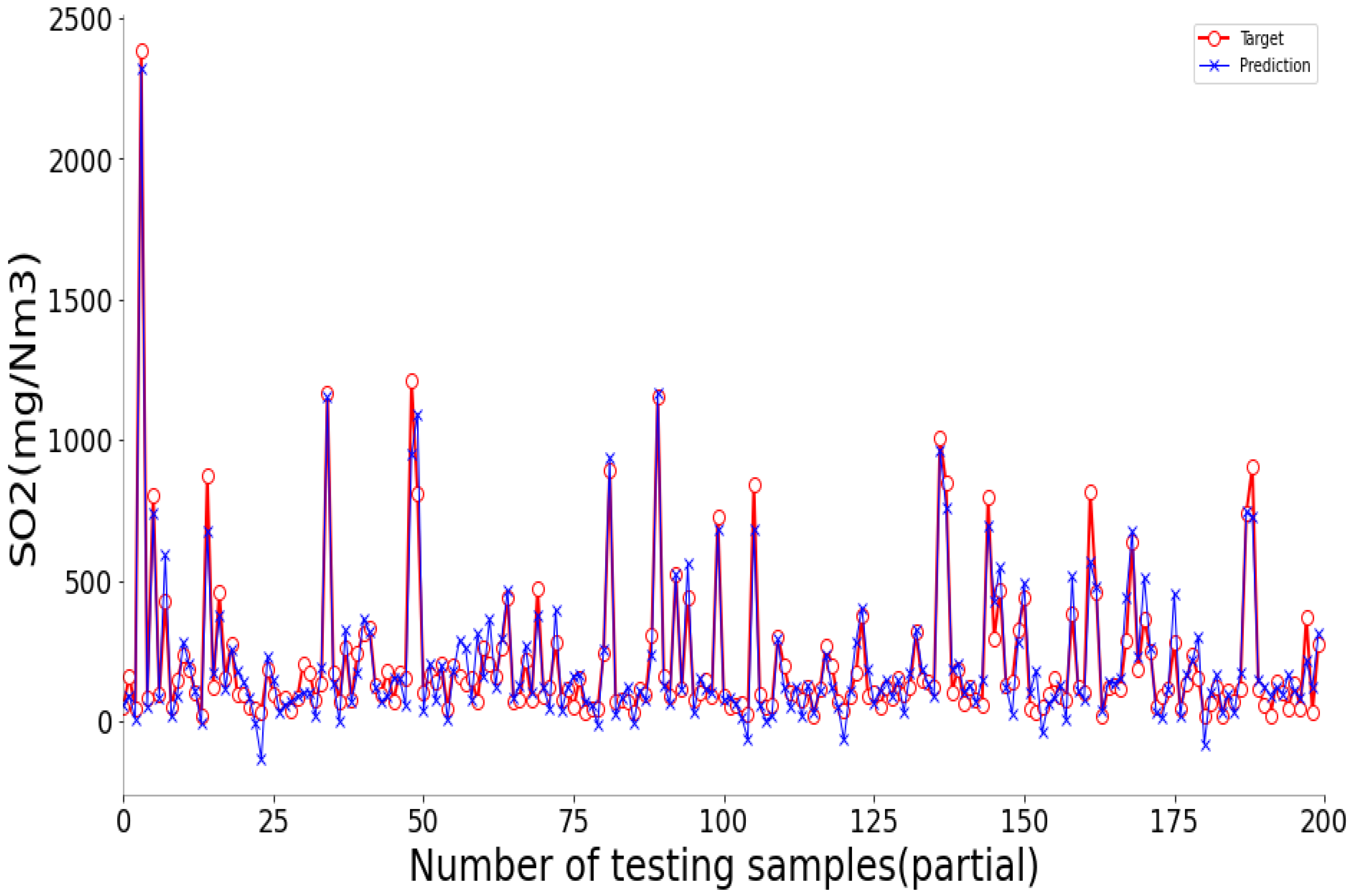
Table 11, compared with RELM, KELM and BLS, the proposed SSA-BLS obtained better model accuracy and model stability in the prediction models established for the NOx emissions concentration and thermal efficiency of CFBB both on the training set and testing set. However, its model prediction accuracy for the SO2 emission concentration of CFBB was not as good as that of KELM.
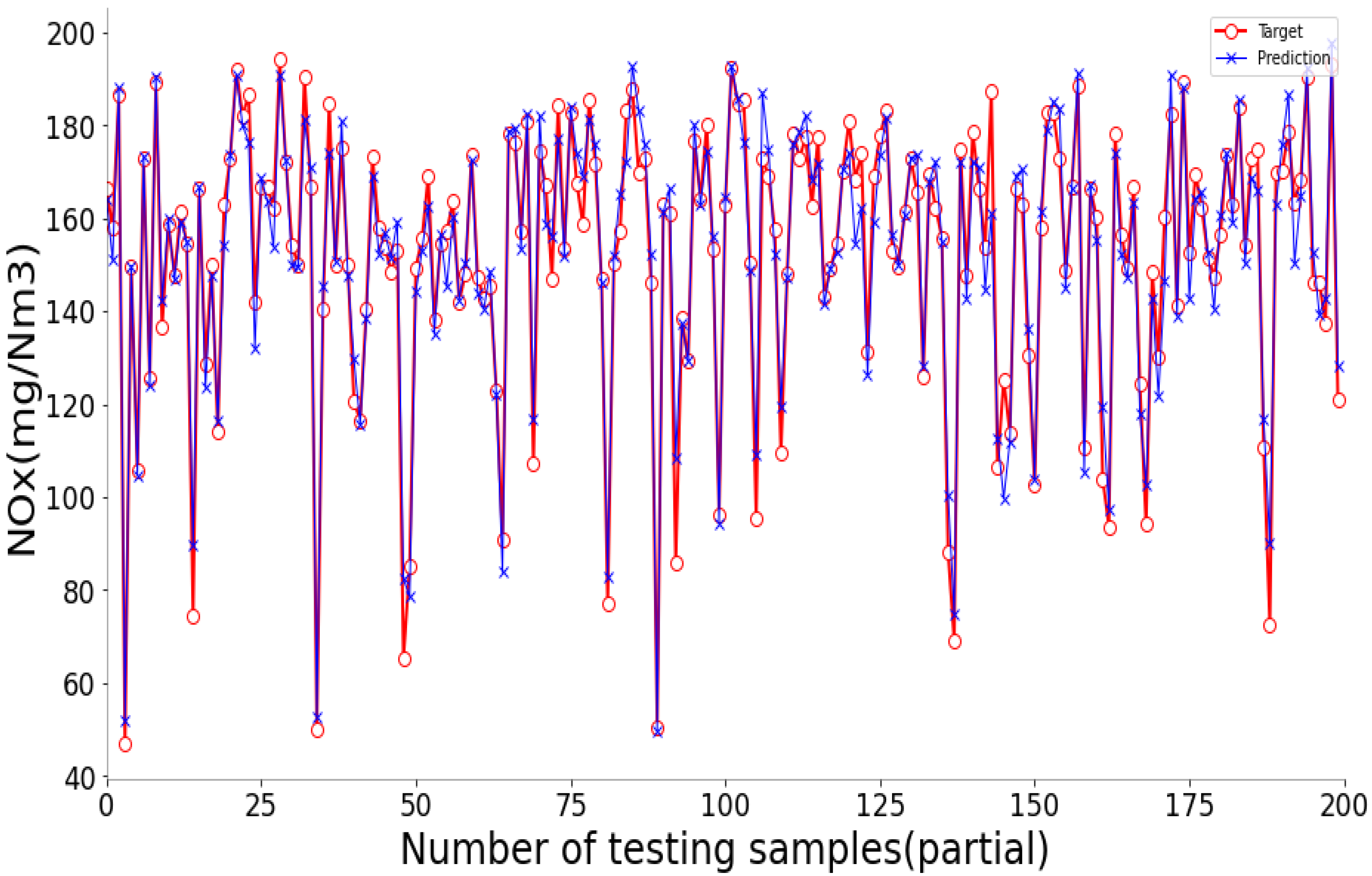
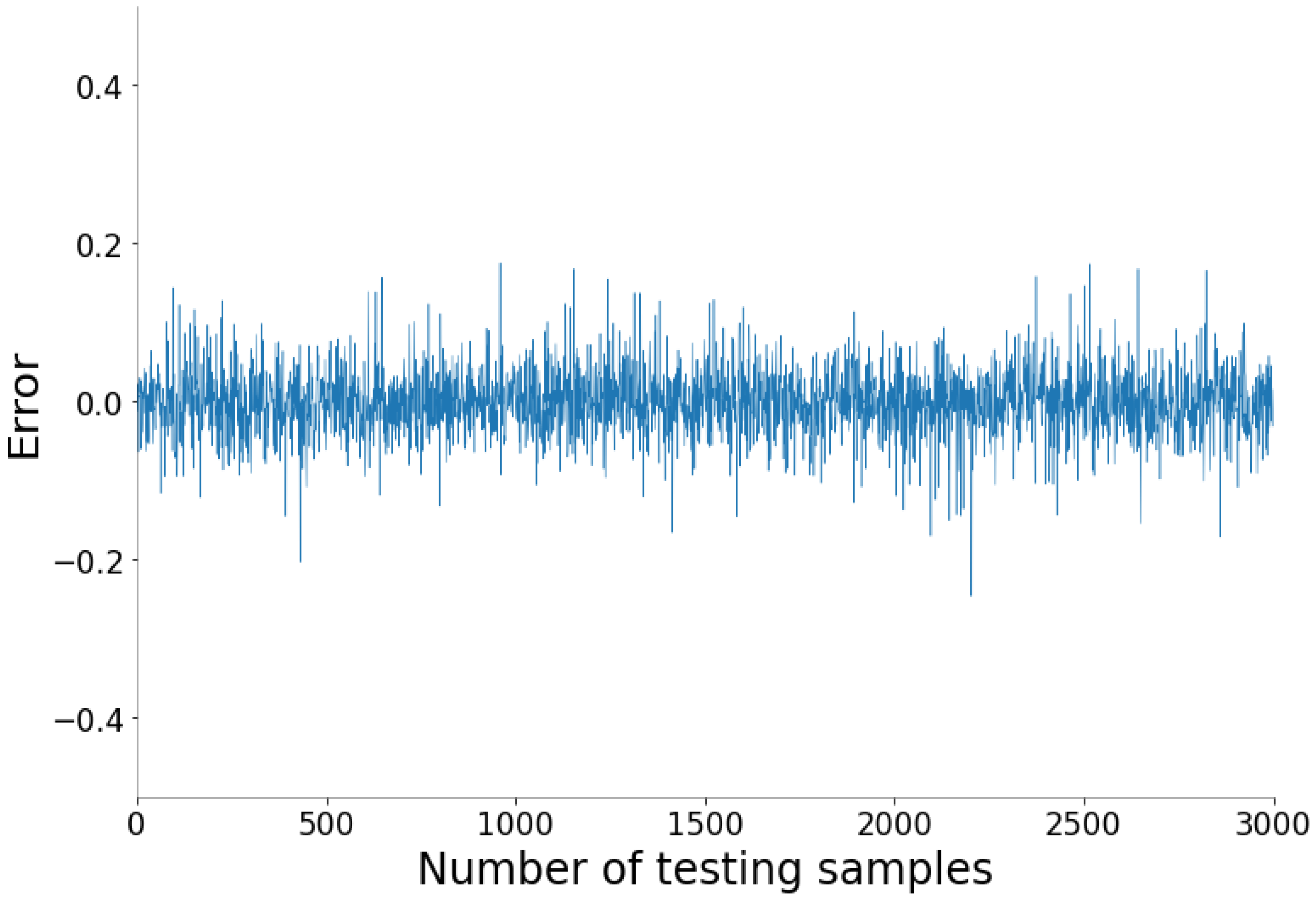
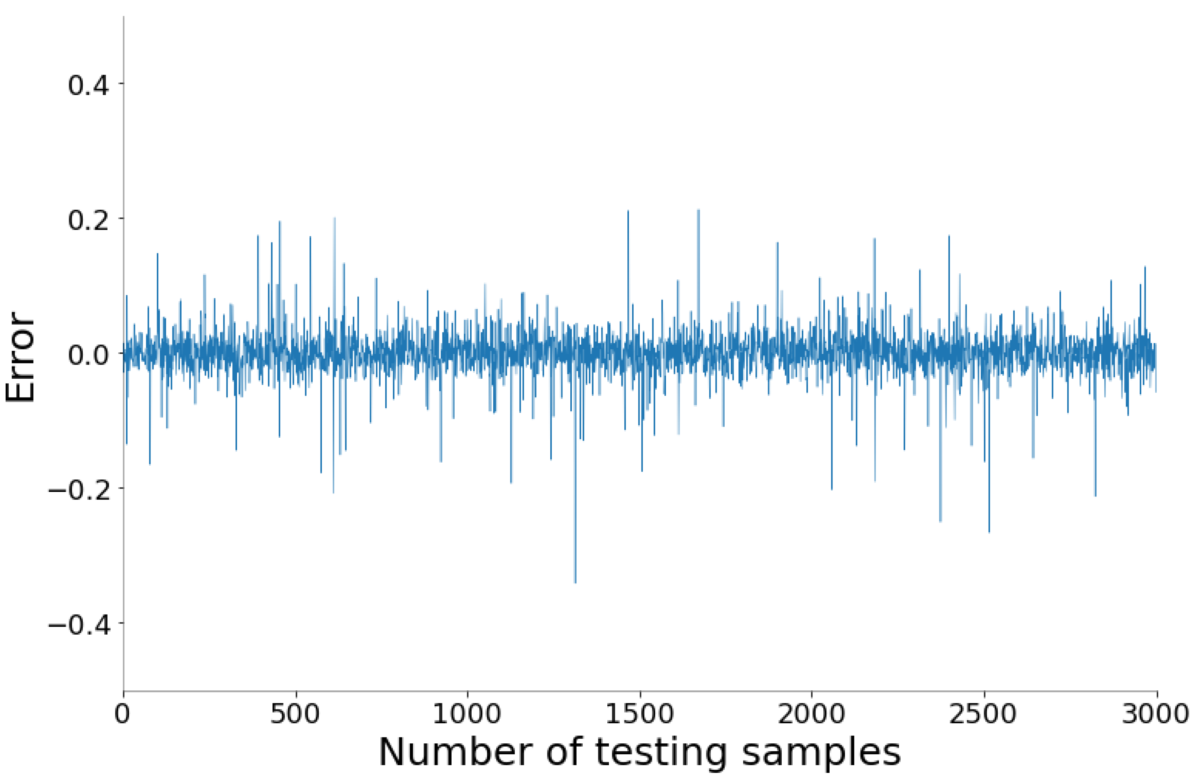
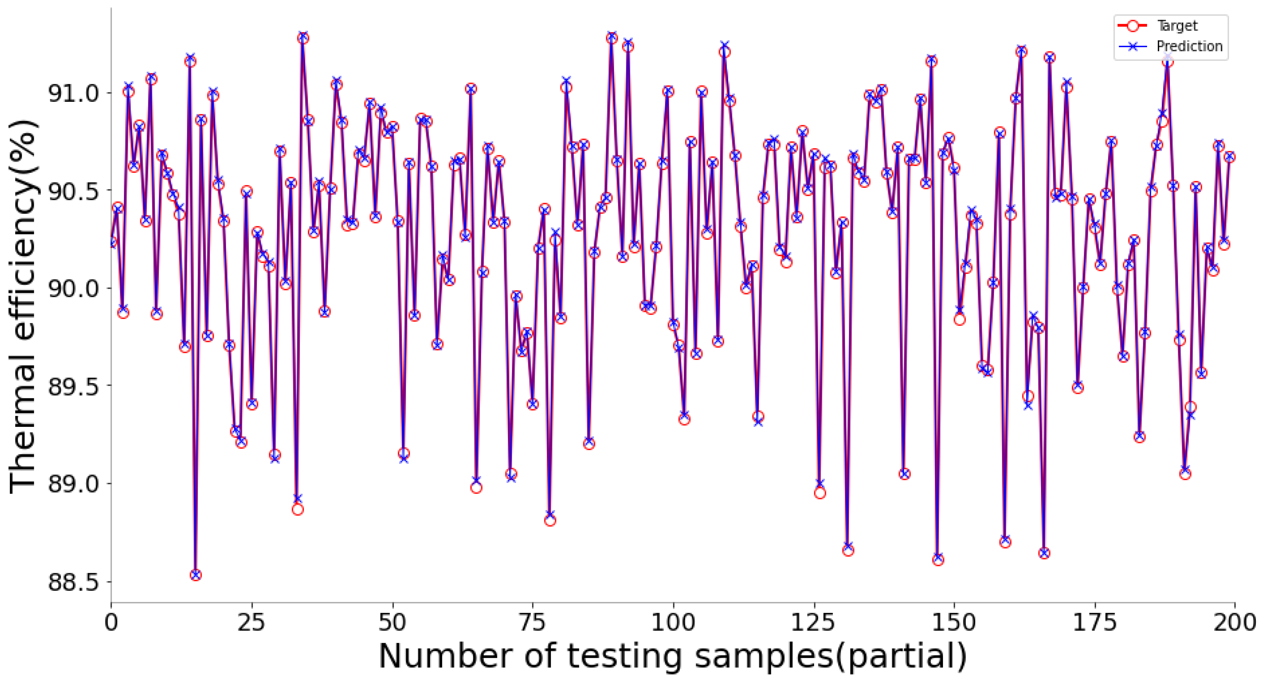
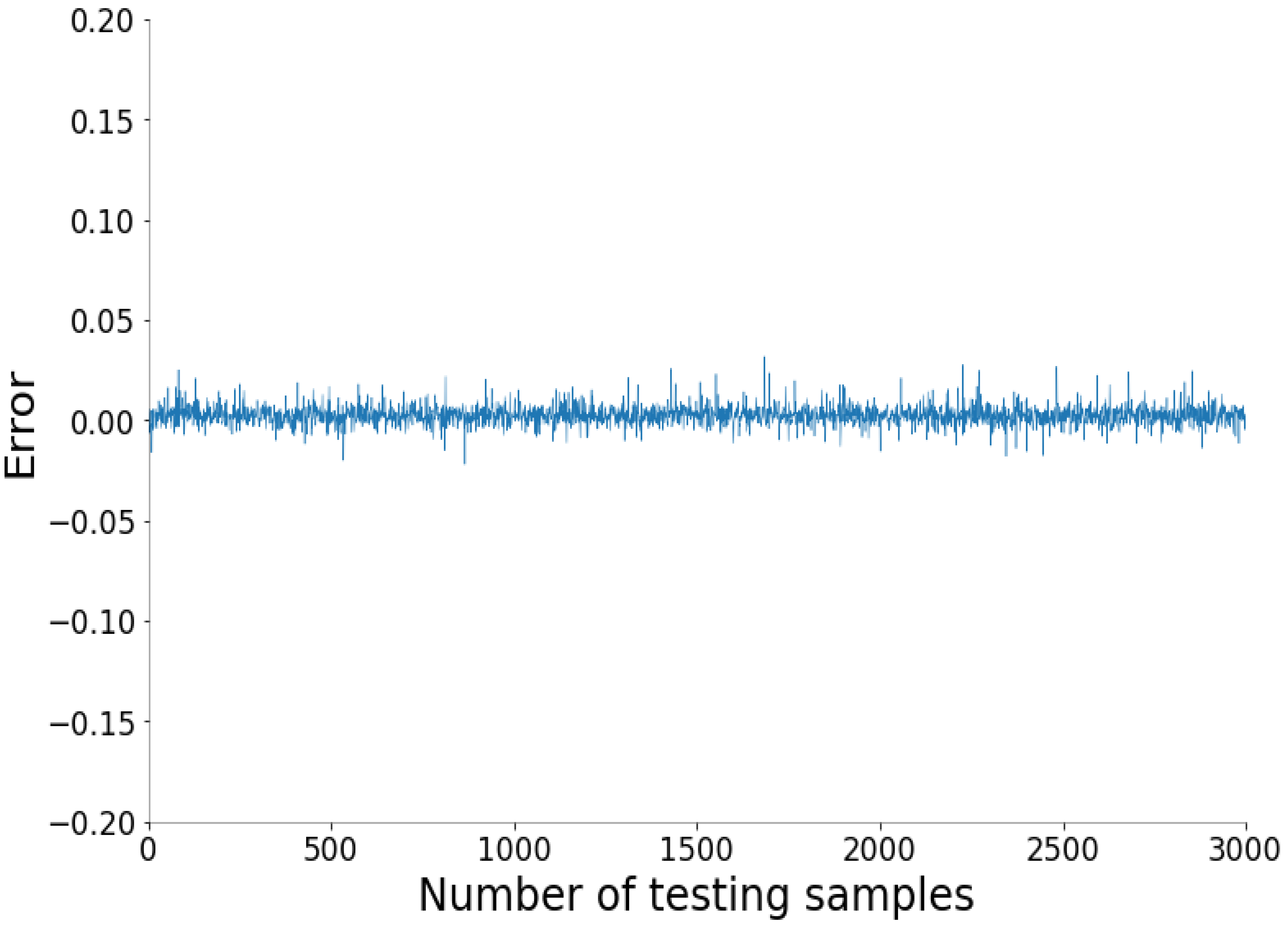
The fitting diagrams and error diagrams of SSA-BLS for modeling the three objectives of CFBB on the testing set are shown in Figure 4, Figure 5, Figure 6, Figure 7, Figure 8 and Figure 9, where the red line and the blue line in the fitting diagram indicate the true values and predicted values of the partial testing set, and the curve in the error diagram represent the error of the predicted values compared to the true values for the testing set.
As shown in Figure 4, Figure 5, Figure 6, Figure 7, Figure 8 and Figure 9, the proposed SSA-BLS effectively establishes the prediction models for the three objectives of CFBB. The three prediction models all have great fitting effect and small fitting error on the testing set.

6. Conclusions

This paper proposed a novel optimized broad learning system by combining with a sparrow search algorithm. That is to say, the sparrow search algorithm was used to optimize the hyper-parameters of broad learning systems. Compared with other state-of-the-art methods, the proposed SSA-BLS reveals better regression accuracy and model stability on testing ten benchmark datasets. Additionally, the SSA-BLS was used to build the collective model of thermal efficiency, NOx and SO2 emissions concentration of one 330MW circulation fluidized bed boiler. Experiment results show that the model accuracy can be achieved 10−2–10−3. The proposed SSA-BLS is an effective modelling method.
However, the proposed SSA-BLS takes more time to determine the optimal hyperparameters. This method improves the accuracy of the model but reduces the speed of model computation. Moreover, this method is also not applicable to online modeling due to the long modeling time. In addition, SSA-BLS only tunes and optimizes the hyperparameters in terms of model accuracy, while ignoring the model stability aspects. In the future, the performance of SSA-BLS will be further improved, including computation speed, model complexity and generalization ability. Additionally, based on the established comprehensive model, we will use one heuristic optimization algorithm to adjust the boiler’s operational parameters for enhancing thermal efficiency and reducing NOx/SO2 emissions concentration.

Author Contributions

Conceptualization, Y.M. and C.X.; methodology, C.X.; software, H.W.; validation, H.W., C.X. and Y.M.; formal analysis, C.X.; investigation, X.G.; resources, Y.M.; data curation, H.W. and C.X.; writing—original draft preparation, C.X.; writing—review and editing, X.G.; visualization, H.W. and C.X.; supervision, R.W.; project administration, S.L.; funding acquisition, Y.M., X.G., R.W. and S.L. All authors have read and agreed to the published version of the manuscript.

Funding

This work is supported by the National Natural Science Foundation of China (Grant No. 62203332) and the Natural Science Foundation of Tianjin (Grant No. 20JCQNJC00430) and the Special fund Project of Tianjin Technology Innovation Guidance (grand No. 21YDTPJC00370) and College Students’ Innovative Entrepreneurial Training Plan Program (Grant No. 202110069034, 202110069003).

Institutional Review Board Statement

Not applicable.

Informed Consent Statement

Not applicable.

Data Availability Statement

The data presented in this study are available on request from the corresponding author. The data are not publicly available due to privacy restriction.

Conflicts of Interest

The authors declare no conflict of interest.

References

  1. Yip, I. Cost analysis of power generation in coal-fired thermal power plants under market economy. Guangdong Electr. Power 2002, 15, 5. [Google Scholar]
  2. Zhou, H. Study of Some Key Issues in NOx Control and Combustion Optimization of Large Power Plant Boilers. Ph.D. Thesis, Zhejiang University, Hangzhou, China, 2004. [Google Scholar]
  3. Cristianini, N.; Shawe-Taylor, J. An Introduction to Support Vector Machines and Other Kernel-Based Learning Methods; Cambridge University Press: Cambridge, UK, 2000. [Google Scholar]
  4. Steinwart, I.; Christmann, A. Support Vector Machines; Information Science and Statistics; Springer: New York, NY, USA, 2008. [Google Scholar]
  5. Zhou, H.; Zhu, H.; Cen, K. A real-time combustion optimization system for thermal power plant boilers based on artificial neural network and genetic algorithm. Power Eng. 2003, 23, 5. [Google Scholar]
  6. Zheng, L.; Zhou, H.; Cen, K.; Wang, C. A comparative study of optimization algorithms for low NOx combustion modification at a coal-fired utility boiler. Expert Syst. Appl. 2009, 36, 2780–2793. [Google Scholar] [CrossRef]
  7. Wu, F.; Zhou, H.; Ren, T.; Zheng, L.; Cen, K. Combining support vector regression and cellular genetic algorithm for multi-objective optimization of coal-fired utility boilers. Fuel 2009, 88, 1864–1870. [Google Scholar] [CrossRef]
  8. Zhou, H.; Zheng, L.; Cen, K. Computational intelligence approach for NOx emissions minimization in a coal-fired utility boiler. Energy Convers. Manag. 2010, 51, 580–586. [Google Scholar] [CrossRef]
  9. Zhou, H.; Zhao, J.; Zheng, L.; Wang, C.; Cen, K. Modeling NOx emissions from coal-fired utility boilers using support vector regression with ant colony optimization. Eng. Appl. Artif. Intell. 2012, 25, 147–158. [Google Scholar] [CrossRef]
  10. Zhou, H.; Cen, K. Combining Neural Network or Support Vector Machine with Optimization Algorithms to Optimize the Combustion. In Combustion Optimization Based on Computational Intelligence; Springer: Singapore, 2018. [Google Scholar]
  11. López-Ibáñez, M. Ant Colony Optimization. In Proceedings of the 12th Annual Conference Companion on Genetic and Evolutionary Computation, GECCO ‘10, Portland, OR, USA, 7–11 July 2010. [Google Scholar]
  12. Huang, G.; Zhu, Q.; Siew, C.K. Extreme Learning Machine: A New Learning Scheme of Feedforward Neural Networks. In Proceedings of the 2004 IEEE International Joint Conference on Neural Networks (IEEE Cat. No.04CH37541), Budapest, Hungary, 25–29 July 2004; Volume 2, pp. 985–990. [Google Scholar]
  13. Huang, G.; Zhu, Q.; Siew, C.K. Extreme learning machine: Theory and applications. Neurocomputing 2006, 70, 489–501. [Google Scholar] [CrossRef]
  14. Huang, G.; Zhou, H.; Ding, X.; Zhang, R. Extreme Learning Machine for Regression and Multiclass Classification. IEEE Trans. Syst. Man Cybern. Part B Cybern. 2012, 42, 513–529. [Google Scholar] [CrossRef] [Green Version]
  15. Li, G.; Niu, P.; Ma, Y.; Wang, H.; Zhang, W. Tuning extreme learning machine by an improved artificial bee colony to model and optimize the boiler efficiency. Knowl. Based Syst. 2014, 67, 278–289. [Google Scholar] [CrossRef]
  16. Li, G.; Niu, P. Combustion optimization of a coal-fired boiler with double linear fast learning network. Soft Comput. 2016, 20, 149–156. [Google Scholar] [CrossRef]
  17. Li, G.; Niu, P.; Duan, X.; Zhang, X. Fast learning network: A novel artificial neural network with a fast learning speed. Neural Comput. Appl. 2013, 24, 1683–1695. [Google Scholar] [CrossRef]
  18. Li, G.; Niu, P.; Wang, H.; Liu, Y. Least Square Fast Learning Network for modeling the combustion efficiency of a 300WM coal-fired boiler. Neural Netw. Off. J. Int. Neural Netw. Soc. 2014, 51, 57–66. [Google Scholar] [CrossRef]
  19. Niu, P.; Ma, Y.; Li, G. Model NOx emission and thermal efficiency of CFBB based on an ameliorated extreme learning machine. Soft Comput. 2018, 22, 4685–4701. [Google Scholar] [CrossRef]
  20. Ma, Y.; Niu, P.; Zhang, X.; Li, G. Research and application of quantum-inspired double parallel feed-forward neural network. Knowl. Based Syst. 2017, 136, 140–149. [Google Scholar] [CrossRef]
  21. Ma, Y.; Niu, P.; Yan, S.; Li, G. A modified online sequential extreme learning machine for building circulation fluidized bed boiler’s NOx emission model. Appl. Math. Comput. 2018, 334, 214–226. [Google Scholar] [CrossRef]
  22. Chen, C.L.; Liu, Z. Broad Learning System: An Effective and Efficient Incremental Learning System Without the Need for Deep Architecture. IEEE Trans. Neural Netw. Learn. Syst. 2018, 29, 10–24. [Google Scholar] [CrossRef]
  23. Hinton, G.E.; Osindero, S.; Teh, Y.W. A Fast-Learning Algorithm for Deep Belief Nets. Neural Comput. 2006, 18, 1527–1554. [Google Scholar] [CrossRef]
  24. Salakhutdinov, R.; Hinton, G.E. Deep Boltzmann Machines. In Proceedings of the 12th International Conference on Artificial Intelligence and Statistics (AISTATS), Clearwater Beach, FL, USA, 16–18 April 2009. [Google Scholar]
  25. Simonyan, K.; Zisserman, A. Very Deep Convolutional Networks for Large-Scale Image Recognition. arXiv 2015, arXiv:1409.1556. [Google Scholar]
  26. Chen, C.L.; Liu, Z.; Feng, S. Universal Approximation Capability of Broad Learning System and Its Structural Variations. IEEE Trans. Neural Netw. Learn. Syst. 2019, 30, 1191–1204. [Google Scholar] [CrossRef]
  27. Jin, J.; Chen, C.L. Robust Broad Learning System for Uncertain Data Modeling. In Proceedings of the 2018 IEEE International Conference on Systems, Man, and Cybernetics (SMC), Miyazaki, Japan, 7–10 October 2018; pp. 3524–3529. [Google Scholar]
  28. Xu, M.; Han, M.; Chen, C.L.; Qiu, T. Recurrent Broad Learning Systems for Time Series Prediction. IEEE Trans. Cybern. 2020, 50, 1405–1417. [Google Scholar] [CrossRef]
  29. Huang, H.; Zhang, T.; Yang, C.; Chen, C.L. Motor Learning and Generalization Using Broad Learning Adaptive Neural Control. IEEE Trans. Ind. Electron. 2020, 67, 8608–8617. [Google Scholar] [CrossRef]
  30. Pu, X.; Li, C. Online Semisupervised Broad Learning System for Industrial Fault Diagnosis. IEEE Trans. Ind. Inform. 2021, 17, 6644–6654. [Google Scholar] [CrossRef]
  31. Liu, Z.; Huang, S.; Jin, W.; Mu, Y. Broad Learning System for semi-supervised learning. Neurocomputing 2021, 444, 38–47. [Google Scholar] [CrossRef]
  32. Zheng, Y.; Chen, B.; Wang, S.; Wang, W. Broad Learning System Based on Maximum Correntropy Criterion. IEEE Trans. Neural Netw. Learn. Syst. 2021, 32, 3083–3097. [Google Scholar] [CrossRef]
  33. Feng, S.; Chen, C.L. Fuzzy Broad Learning System: A Novel Neuro-Fuzzy Model for Regression and Classification. IEEE Trans. Cybern. 2020, 50, 414–424. [Google Scholar] [CrossRef]
  34. Zhao, H.; Zheng, J.; Deng, W.; Song, Y. Semi-Supervised Broad Learning System Based on Manifold Regularization and Broad Network. In IEEE Transactions on Circuits and Systems I: Regular Papers; IEEE: Manhattan, NY, USA, 2020; Volume 67, pp. 983–994. [Google Scholar]
  35. Nacef, A.; Kaci, A.; Aklouf, Y.; Dutra, D.L. Machine learning based fast self optimized and life cycle management network. Comput. Netw. 2022, 209, 108895. [Google Scholar] [CrossRef]
  36. Ali, A.; Irshad, K.; Khan, M.F.; Hossain, M.M.; Al-Duais, I.N.; Malik, M.Z. Artificial Intelligence and Bio-Inspired Soft Computing-Based Maximum Power Plant Tracking for a Solar Photovoltaic System under Non-Uniform Solar Irradiance Shading Conditions—A Review. Sustainability 2021, 13, 10575. [Google Scholar] [CrossRef]
  37. Xue, J.; Shen, B. A novel swarm intelligence optimization approach: Sparrow Search Algorithm. Syst. Sci. Control. Eng. 2020, 8, 22–34. [Google Scholar] [CrossRef]
  38. Poli, R.; Kennedy, J.; Blackwell, T.M. Particle swarm optimization. Swarm Intell. 2007, 1, 33–57. [Google Scholar] [CrossRef]
  39. Trelea, I.C. The particle swarm optimization algorithm: Convergence analysis and parameter selection. Inf. Process. Lett. 2003, 85, 317–325. [Google Scholar] [CrossRef]
  40. Rashedi, E.; Nezamabadi-Pour, H.; Saryazdi, S. GSA: A Gravitational Search Algorithm. Inf. Sci. 2009, 179, 2232–2248. [Google Scholar] [CrossRef]
  41. Mirjalili, S.M.; Mirjalili, S.M.; Lewis, A. Grey Wolf Optimizer. Adv. Eng. Softw. 2014, 69, 46–61. [Google Scholar] [CrossRef] [Green Version]
  42. Saud, S.J.; Jamil, B.; Upadhyay, Y.; Irshad, K. Performance improvement of empirical models for estimation of global solar radiation in India: A k-fold cross-validation approach. Sustain. Energy Technol. Assess. 2020, 40, 100768. [Google Scholar] [CrossRef]
  43. Zheng, W.; Qian, Y.; Lu, H. Text categorization based on regularization extreme learning machine. Neural Comput. Appl. 2011, 22, 447–456. [Google Scholar] [CrossRef]
  44. Wang, M.; Chen, H.; Yang, B.; Zhao, X.; Hu, L.; Cai, Z.; Huang, H.; Tong, C. Toward an optimal kernel extreme learning machine using a chaotic moth-flame optimization strategy with applications in medical diagnoses. Neurocomputing 2017, 267, 69–84. [Google Scholar] [CrossRef]
  45. Chen, H.; Zhang, Q.; Luo, J.; Xu, Y.; Zhang, X. An enhanced Bacterial Foraging Optimization and its application for training kernel extreme learning machine. Appl. Soft Comput. 2020, 86, 105884. [Google Scholar] [CrossRef]
  46. Parvandeh, S.; Yeh, H.; Paulus, M.P.; McKinney, B.A. Consensus features nested cross-validation. Bioinformatics 2020, 36, 3093–3098. [Google Scholar] [CrossRef]
  47. Pao, Y.; Takefuji, Y. Functional-link net computing: Theory, system architecture, and functionalities. Computer 1992, 25, 76–79. [Google Scholar] [CrossRef]
  48. Pao, Y.; Park, G.H.; Sobajic, D.J. Learning and generalization characteristics of the random vector Functional-link net. Neurocomputing 1994, 6, 163–180. [Google Scholar] [CrossRef]
  49. Igelnik, B.; Pao, Y. Stochastic choice of basic functions in adaptive function approximation and the functional-link net. IEEE Trans. Neural Netw. 1995, 6, 1320–1329. [Google Scholar] [CrossRef]
Figure 1. The structure diagram of BLS.
Energies 15 07700 g001
Figure 2. The schematic diagram of the fitness value calculating process, k is the number of cross-validations.
Energies 15 07700 g002
Figure 3. The flowchart of SSA-BLS.
Energies 15 07700 g003
Figure 4. The fitting diagram of NOx emission concentration model.
Energies 15 07700 g004
Figure 5. The error diagram of NOx emission concentration model.
Energies 15 07700 g005
Figure 6. The fitting diagram of SO2 emission concentration model.
Energies 15 07700 g006
Figure 7. The error diagram of SO2 emission concentration model.
Energies 15 07700 g007
Figure 8. The fitting diagram of thermal efficiency model.
Energies 15 07700 g008
Figure 9. The error diagram of thermal efficiency model.
Energies 15 07700 g009
Table 1. Description of regression data sets.
DatasetsAttributesInstancesTraining SamplesTesting Samples
Gasoline octane1432422797
Fuel consumption131067747320
Auto MPG7392274118
Abalone8417729231254
Bank domains8819231491350
Boston housing13506354152
Delta elevators6951766612856
Forest fires12517361156
Machine CPU620914663
Servo416711651
Table 2. The optimization range of hyper-parameter combination.
Hyper-ParametersMeaningOptimal Scope
N f Number of feature nodes[1, 20]
N m Number of feature mapping groups[1, 40]
N e Number of enhanced nodes[1, 500]
Table 3. The RMSE of the four algorithms on the training set.
DatasetsRELMKELMBLSSSA-BLS
RMSERMSERMSERMSE
AVGSDAVGSDAVGSDAVGSD
Gasoline octane 4.47 × 10−29.02 × 10−33.83 × 10−27.99 × 10−33.86 × 10−28.16 × 10−33.78 × 10−28.16 × 10−3
Fuel consumption2.47 × 10−28.38 × 10−41.79 × 10−21.49 × 10−44.09 × 10−21.76 × 10−39.93 × 10−32.37 × 10⁻³
Auto MPG1.42 × 10−45.04 × 10−51.00 × 10−51.34 × 10−75.75 × 10−53.49 × 10−51.04 × 10−53.50 × 10⁻⁵
Abalone1.38 × 10−58.43 × 10−62.70 × 10−64.41 × 10−84.06 × 10−35.37 × 10−34.82 × 10−87.11 × 10⁻⁸
Bank domains3.01 × 10−43.47 × 10−54.13 × 10−62.57 × 10−85.57 × 10−53.32 × 10−57.59 × 10−97.82 × 10⁻⁹
Boston housing7.23 × 10−41.72 × 10−46.83 × 10−66.83 × 10−81.86 × 10−51.07 × 10−59.89 × 10−86.25 × 10⁻⁸
Delta elevators5.28 × 10−71.02 × 10−72.32 × 10−83.41 × 10−102.08 × 10−71.61 × 10−73.85 × 10−93.42 × 10−9
Forest fires3.32 × 10−46.63 × 10−55.97 × 10−56.15 × 10−72.24 × 10−41.61 × 10−42.93 × 10−71.44 × 10⁻⁷
Machine CPU1.33 × 10−41.52 × 10−43.42 × 10−53.56 × 10−68.86 × 10−75.15 × 10−72.57 × 10−81.28 × 10⁻⁸
Servo1.44 × 10−45.06 × 10−53.70 × 10−53.96 × 10−76.42 × 10−45.02 × 10−43.83 × 10−72.87 × 10⁻⁷
Table 4. The RMSE of the four algorithms on the testing set.
DatasetsRELMKELMBLSSSA-BLS
RMSERMSERMSERMSE
AVGSDAVGSDAVGSDAVGSD
Gasoline octane7.16 × 10−29.68 × 10−32.70 × 10−23.09 × 10−23.04 × 10−23.20 × 10−22.65 × 10−23.07 × 10⁻²
Fuel consumption2.64 × 10−21.26 × 10−32.09 × 10−23.43 × 10−34.85 × 10−22.79 × 10−31.39 × 10−22.84 × 10⁻³
Auto MPG2.06 × 10−45.65 × 10−51.09 × 10−52.18 × 10−65.82 × 10−53.58 × 10−51.19 × 10−53.06 × 10⁻⁵
Abalone1.71 × 10−57.95 × 10−62.86 × 10−65.16 × 10−64.18 × 10−35.76 × 10−38.34 × 10−81.80 × 10⁻⁷
Bank domains3.34 × 10−43.02 × 10−54.27 × 10−62.69 × 10−71.94 × 10−44.13 × 10−47.79 × 10−98.32 × 10⁻⁹
Boston housing2.11 × 10−37.65 × 10−47.40 × 10−61.83 × 10−61.85 × 10−51.08 × 10−59.69 × 10−86.07 × 10⁻⁸
Delta elevators6.18 × 10−71.26 × 10−73.04 × 10−86.40 × 10−92.08 × 10−71.61 × 10−73.85 × 10−93.41 × 10⁻⁹
Forest fires1.99 × 10−31.21 × 10−37.24 × 10−51.45 × 10−52.2 × 10−41.58 × 10−42.94 × 10−71.43 × 10⁻⁷
Machine CPU5.43 × 10−42.41 × 10−47.36 × 10−59.17 × 10−58.13 × 10−75.16 × 10−72.28 × 10−81.61 × 10⁻⁸
Servo1.89 × 10−46.42 × 10−53.22 × 10−51.25 × 10−58.13 × 10−48.62 × 10−43.81 × 10−72.39 × 10⁻⁷
Table 5. The MAPE of the four algorithms on the training set and testing set.
DatasetsRELMKELMBLSSSA-BLS
TrainTestTrainTestTrainTestTrainTest
Gasoline octane8.16 × 10−11.332.573.689.29 × 10−11.009.24 × 10−19.76 × 10⁻¹
Fuel consumption2.562.592.41 × 10−14.16 × 10−12.632.711.092.59
Auto MPG3.30 × 10−23.51 × 10−21.11 × 10−11.17 × 10−16.60 × 10−46.23 × 10−46.26 × 10−48.14 × 10⁻⁴
Abalone2.56 × 10−22.01 × 10−22.00 × 10−22.13 × 10−22.51 × 10−12.56 × 10−12.18 × 10−62.30 × 10⁻⁶
Bank domains3.62 × 10−13.67 × 10−13.68 × 10−23.71 × 10−27.99 × 10−28.04 × 10−29.60 × 10−79.68 × 10⁻⁷
Boston housing9.81 × 10−11.233.86 × 10−24.31 × 10−24.51 × 10−44.57 × 10−48.54 × 10−68.32 × 10⁻⁶
Delta elevators2.51 × 10−22.56 × 10−21.31 × 10−21.31 × 10−23.21 × 10−23.21 × 10−25.04 × 10−45.05 × 10⁻⁴
Forest fires4.78 × 10−16.21 × 10−15.31 × 10−25.61 × 10−21.57 × 10−21.59 × 10−22.13 × 10−52.14 × 10⁻⁵
Machine CPU2.05 × 10−21.27 × 10−11.41 × 10−11.76 × 10−15.73 × 10−55.69 × 10−51.46 × 10−61.47 × 10⁻⁶
Servo2.62 × 10−33.29 × 10−35.95 × 10−26.44 × 10−26.06 × 10−37.91 × 10−31.12 × 10−51.39 × 10⁻⁵
Table 6. Description of variable symbols.
Symbol NameDescription
17ANO037Boiler load
AFCOALQThe first coal feeder coal volume
BFCOALQThe second coal feeder coal volume
CFCOALQThe third coal feeder coal volume
DFCOALQThe fourth coal feeder coal volume
18ANO074Average bed temperature in the upper part of the dense phase zone of the furnace
05F051Primary air flow at the left duct burner inlet
05F061Right duct burner inlet primary air flow
05T457Primary air temperature at the left duct burner inlet
05T467Right duct burner inlet primary air temperature
06F061Total right side secondary air flow
06F052Left side internal secondary air distribution flow
06F062Right side internal secondary air distribution flow
06T453The second secondary fan motor drive end bearing temperature
06T463The first secondary fan motor drive end bearing temperature
17I021The first limestone powder conveying motor current
17I011The second limestone powder conveying motor current
CEMSO2CEMS flue gas O2 concentration
CEMSTEMPCEMS flue gas temperature
08A051Carbon content of fly ash at the inlet of the left EDC
08A061Carbon content of fly ash at the inlet of the right EDC
05T402The first Primary fan inlet temperature
05T403The second Primary fan inlet temperature
12T612The first old slagger outlet temperature
12T622The second cold slagger outlet temperature
12T632The third cold slagger outlet temperature
12T642The fourth cold slagger outlet temperature
CEMSNOXCEMS flue gas NOx concentration
CEMSSO2CEMS flue gas SO2 concentration
TEBoiler thermal efficiency
Table 7. The partial data of a 330MW CFBB operational conditions.
NO.17ANO037AFCOALQBFCOALQCFCOALQDFCOALQ18ANO07405F05105F06105T45705T46706F06106F05206F06206T45306T463
173.40138.06539.17439.12238864.328202.548220.4269.342267.375385.664182.617163.927278.823267.433
273.40138.06539.17439.12238864.328266.631232.072269.342267.375385.31195.301152.674278.823267.433
373.5238.06539.17439.12238864.207249.237263.656269.342267.375435.575178.803171.079278.823267.433
473.5238.06539.17439.12238864.03263.656242.371269.342267.375405.929209.128186.146278.823267.433
573.5237.96239.17439.12237.862863.881298.673248.093269.342267.375402.92183.762177.659278.823267.433
999696.31856.96652.71252.95356.528866.957419.973368.935273.729270.847976.991569.881669.725284.775268.966
999796.42756.96652.55652.95356.528867.103338.267273.955273.729270.847973.451626.621598.299284.775268.966
999896.42756.96652.40352.95356.528867.278386.329349.71273.729270.8471017.08631.294601.922284.775268.966
999996.42756.96652.27352.80156.528867.39405.325343.073273.729270.8471020.796569.118612.603284.775268.966
1000096.42756.96652.27352.68956.528867.557313.549324.306273.729270.8471036.903543.752645.026284.775268.966
NO.17I02117I0116CEMSO26CEMSTEMP08A05108A06105T40205T40312T61212T62212T63212T642CEMSNOXCEMSNOXTE
1102.876116.0745.554152.6550.8470.31625.6524.90142.85845.35551.82936.858128.395225.28590.55405
2103.944114.8155.554152.6550.8470.31625.6524.90142.85845.35551.82936.858128.395224.14190.55405
3103.296113.1755.554152.6550.8470.31625.6524.90142.85845.35551.82936.858128.929223.37890.55405
4103.334114.7015.554152.6550.8470.31625.6524.90142.85845.35551.82936.858129.463220.51790.55405
5104.059113.3285.554152.6550.8470.31625.6524.90142.85845.35551.82936.858129.463218.6190.55405
9996102.914116.6844.921156.6371.4050.16730.23528.19339.12737.04636.84647.32160.436144.99190.30709
9997102.914116.994.921156.6371.4050.16730.23528.19339.12737.04636.84647.32160.436147.08990.30709
9998103.792117.7144.921156.6371.4050.16730.23528.19339.12737.04636.84647.32160.436148.61590.30709
9999102.418115.9984.921156.6371.4050.16730.23528.19339.12737.04636.19247.32160.436150.1490.30709
10000101.541115.7314.921156.6371.4050.16730.23528.19339.12737.04636.19247.32159.826151.66690.30709
Table 8. The hyper-parameters of SSA-BLS and BLS for boiler data modeling.
ObjectivesSSA-BLS
N1N2N3
NOx237478
SO2113459
TE227296
Table 9. The RMSE of the four algorithms on the training set of boiler data.
ObjectivesRELMKELMBLSSSA-BLS
RMSERMSERMSERMSE
AVGSDAVGSDAVGSDAVGSD
NOX9.05 × 10−26.51 × 10−33.48 × 10−24.26 × 10−54.22 × 10−29.50 × 10−42.17 × 10−24.23 × 10⁻⁴
SO28.31 × 10−22.37 × 10−31.99 × 10−21.49 × 10−45.56 × 10−27.12 × 10−43.37 × 10−21.13 × 10⁻³
TE4.52 × 10−21.01 × 10−22.04 × 10−23.36 × 10−55.96 × 10−21.20 × 10−34.41 × 10−31.72 × 10⁻⁴
Table 10. The RMSE of the four algorithms on the testing set of boiler data.
ObjectivesRELMKELMBLSSSA-BLS
RMSERMSERMSERMSE
AVGSDAVGSDAVGSDAVGSD
NOX8.91 × 10−25.94 × 10−37.49 × 10−22.36 × 10−36.53 × 10−26.55 × 10−22.75 × 10−21.83 × 10⁻³
SO27.91 × 10−22.09 × 10−24.12 × 10−25.53 × 10−35.82 × 10−24.98 × 10−33.59 × 10−21.94 × 10⁻³
TE4.48 × 10−29.68 × 10−35.37 × 10−22.85 × 10−36.26 × 10−31.18 × 10−34.58 × 10−31.60 × 10⁻⁴
Table 11. The MAPE of the four algorithms on the training set and testing set of boiler data.
ObjectivesRELMKELMBLSSSA-BLS
TrainingTestingTrainingTestingTraining Testing Training Testing
NOX4.224.131.742.462.202.221.571.83
SO24.144.101.071.203.143.321.922.06
TE2.282.269.26 × 10−21.983.03 × 10−13.09 × 10−12.10 × 10−12.18 × 10⁻¹
Publisher’s Note: MDPI stays neutral with regard to jurisdictional claims in published maps and institutional affiliations.

