
Voltage Stability Control Based on Angular Indexes from Stationary Analysis

Abstract
:1. Introduction
2. Voltage Stability, Controls, and Indexes
2.1. Power-System Voltage Stability
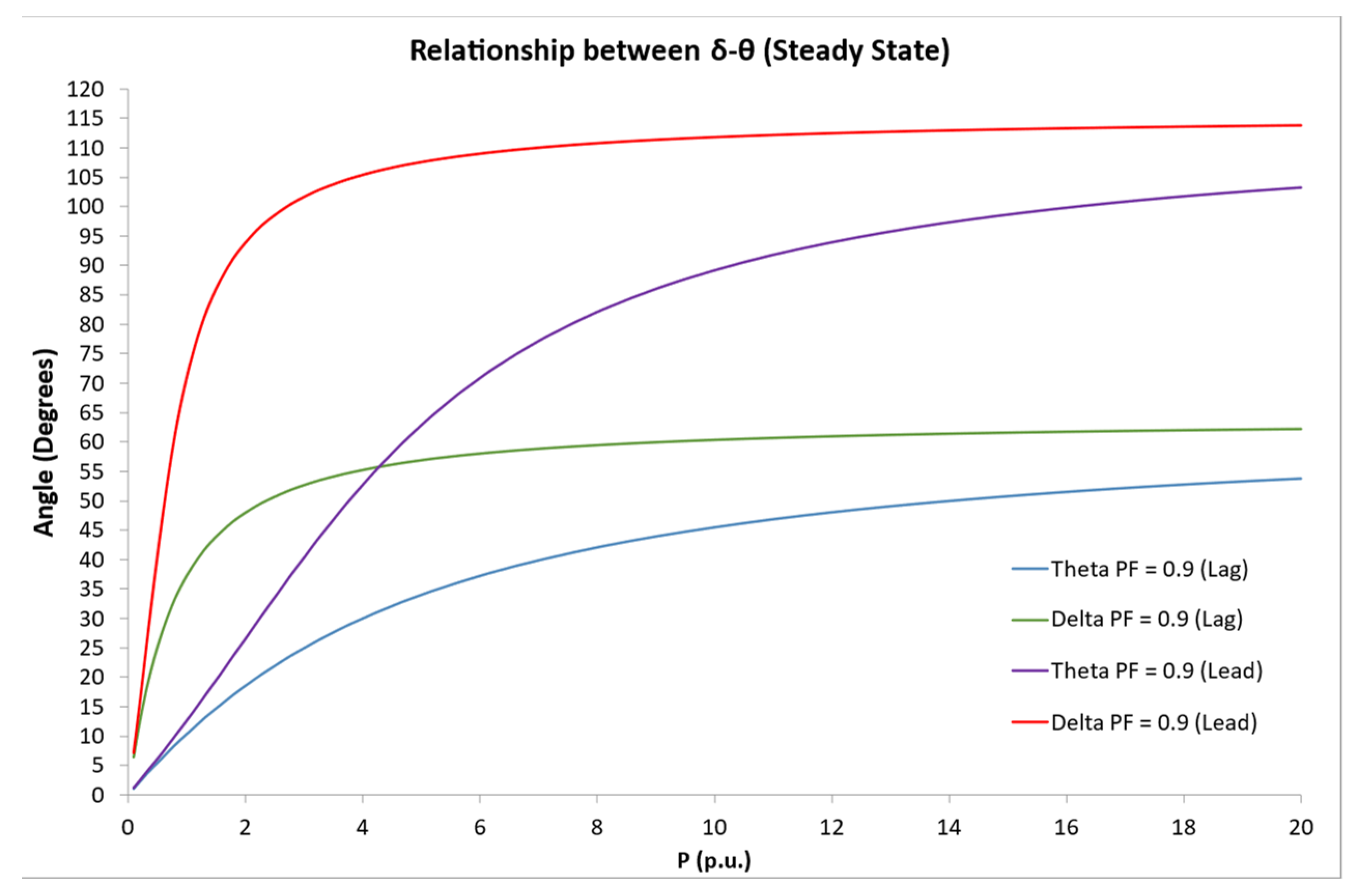
2.2. Angular Indexes
3. Angular Characterization Methodology with Stationary Analysis
3.1. Stage 1
3.2. Stage 2
3.3. Stage 3
4. Application of Angular Characterization Methodology to the IEEE 39-Bus System
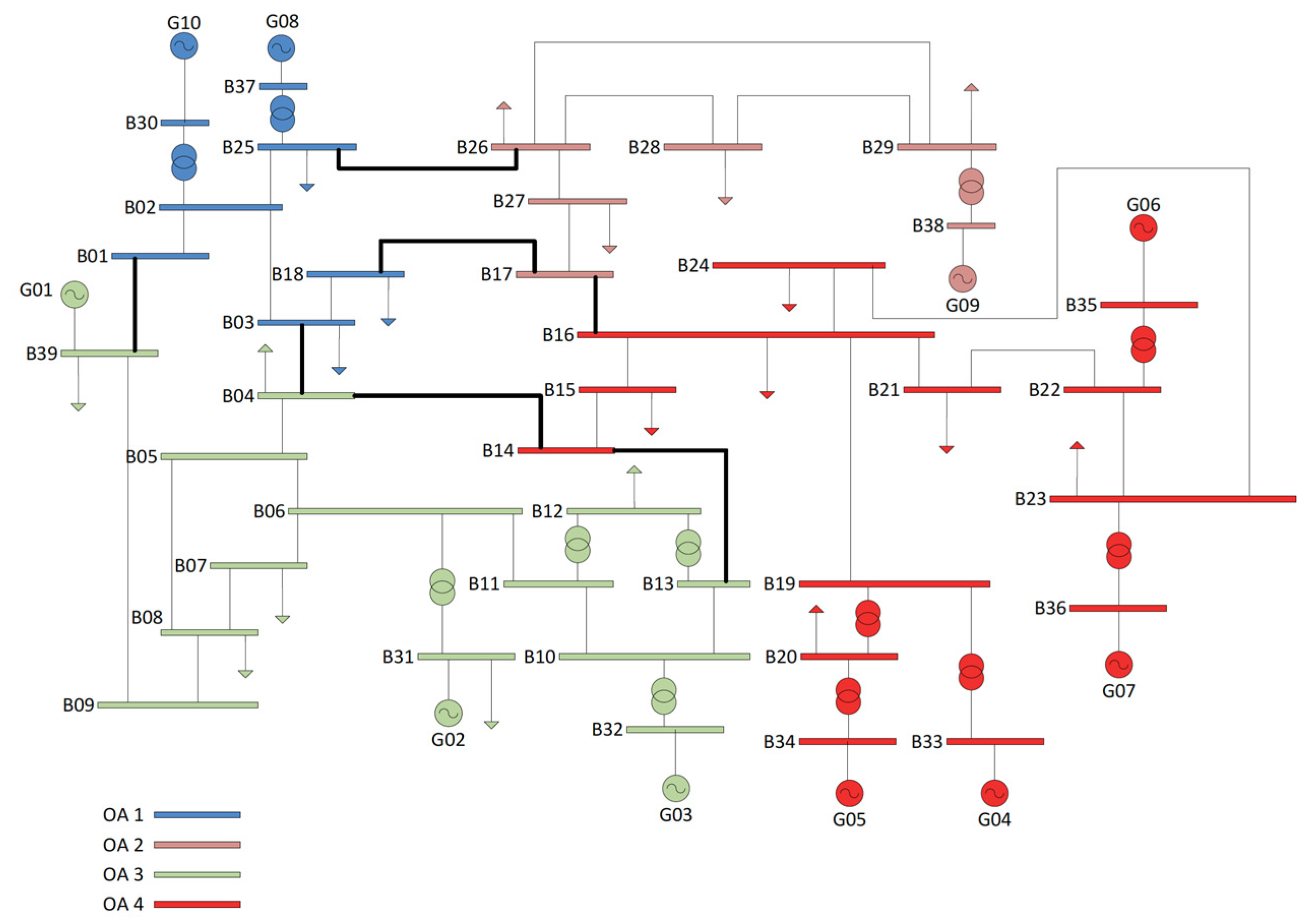
4.1. IEEE 39-Bus System
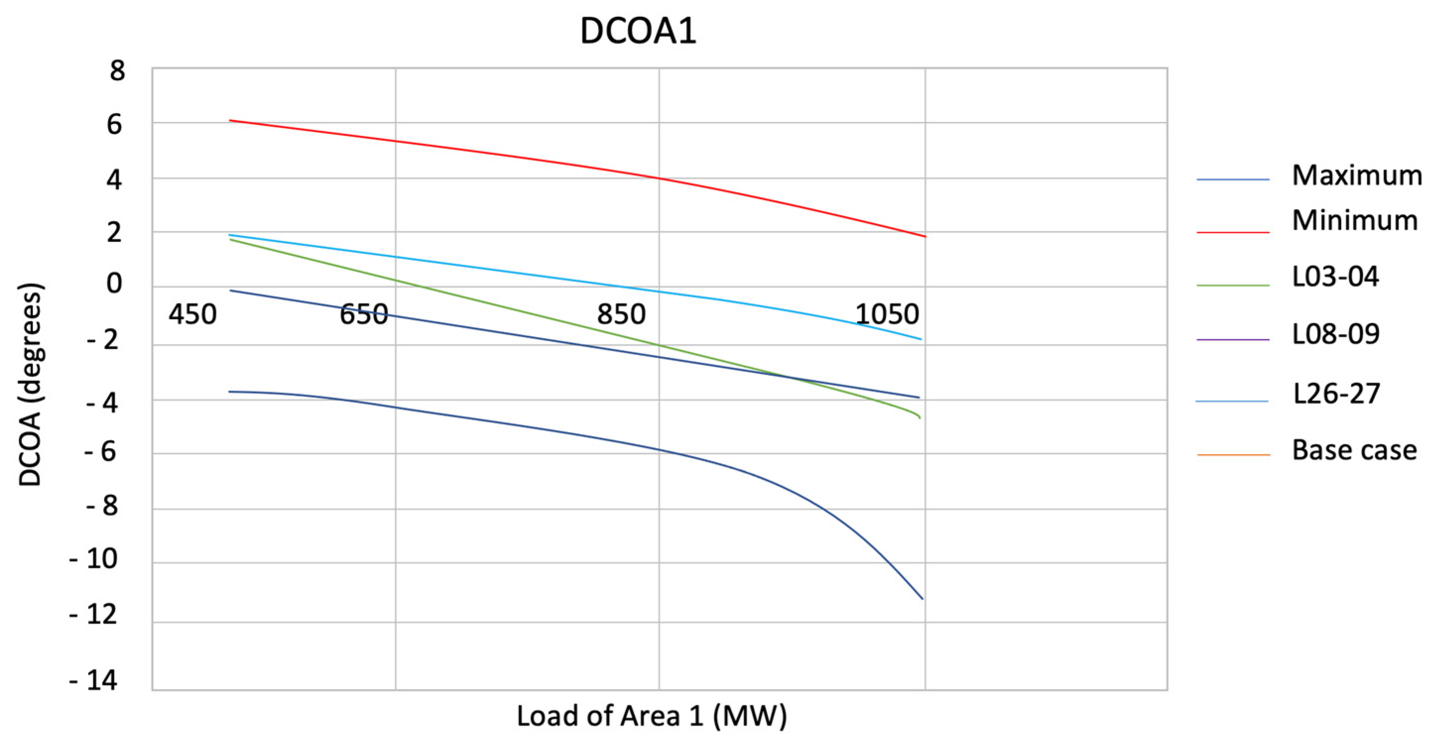
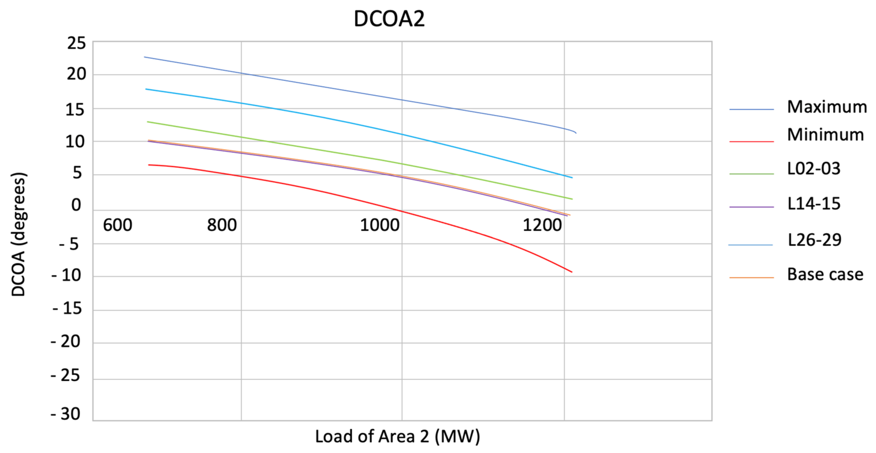
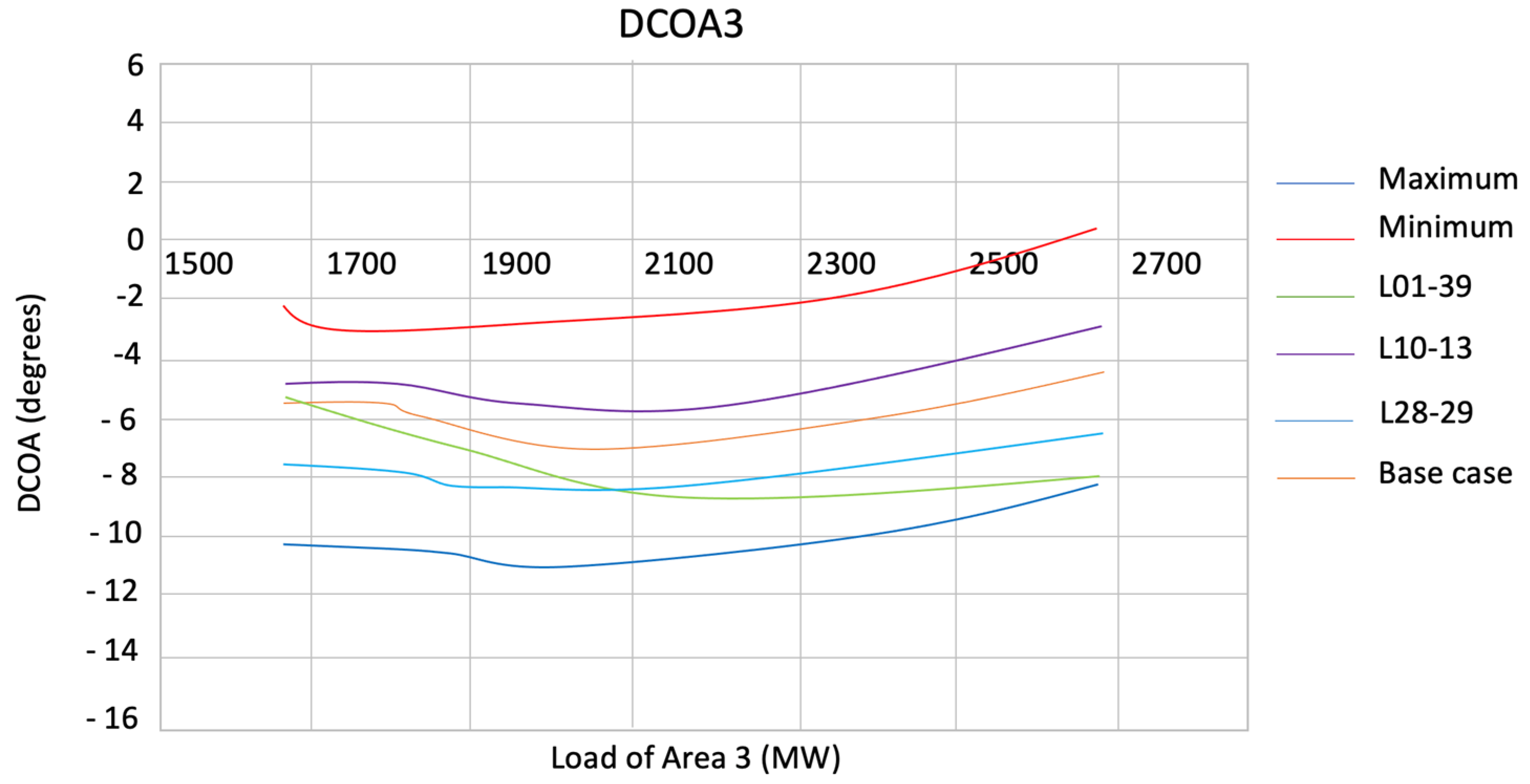
4.2. Angular Characterization in IEEE 39-Bus System
5. Angular Characterization Methodology with Stationary Analysis
5.1. Stage 1
5.2. Stage 2
5.3. Stage 3
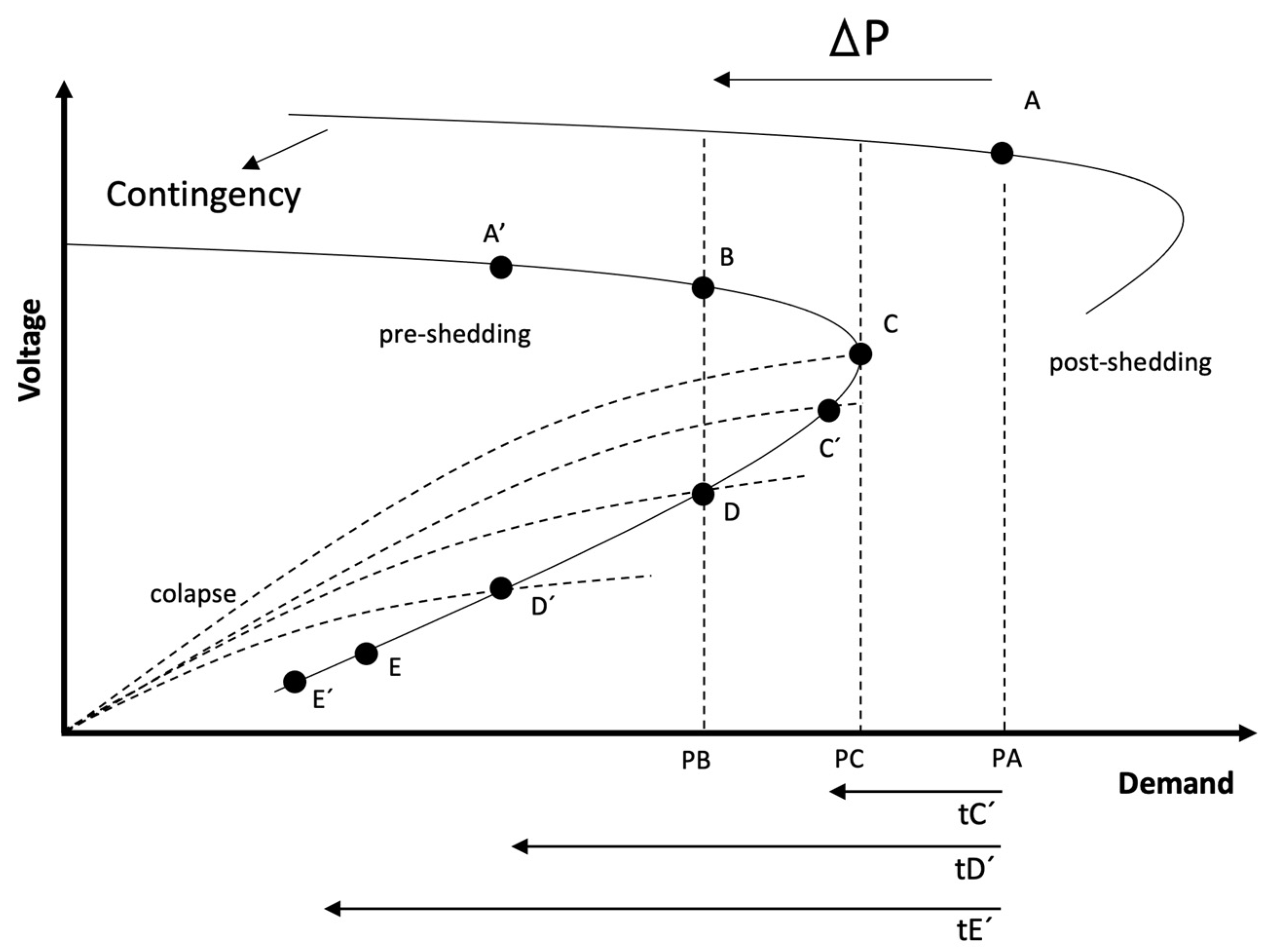
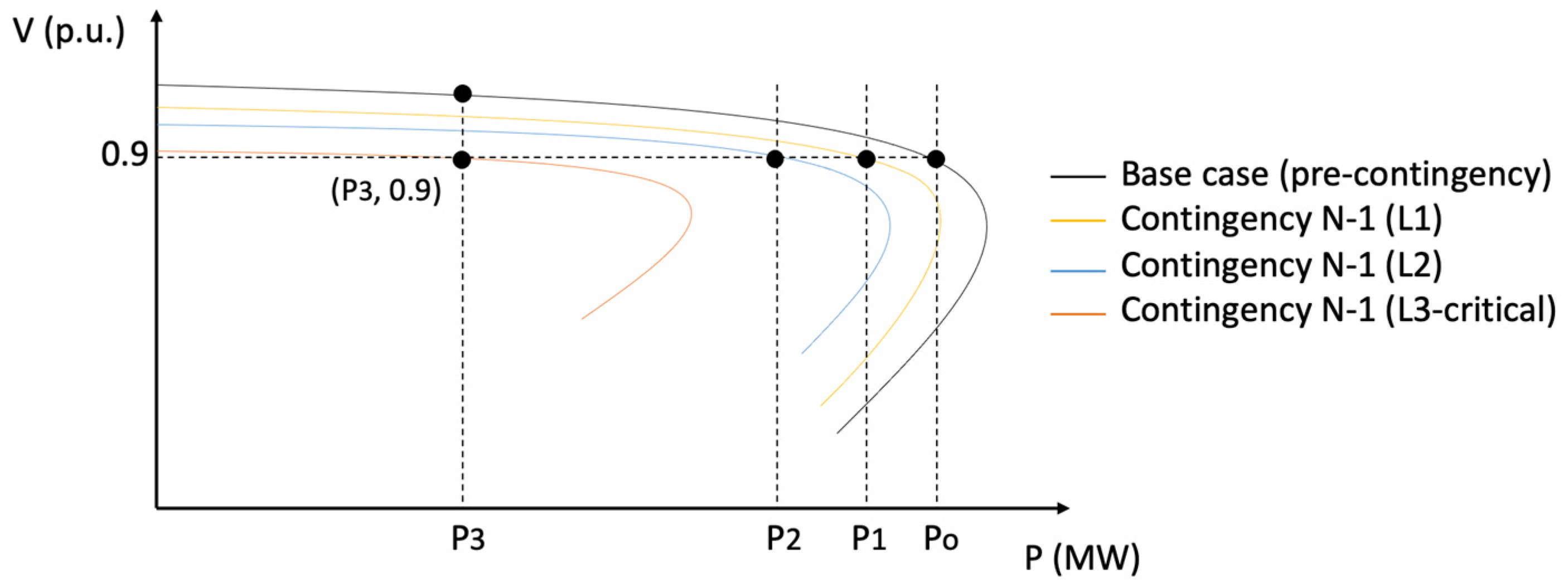
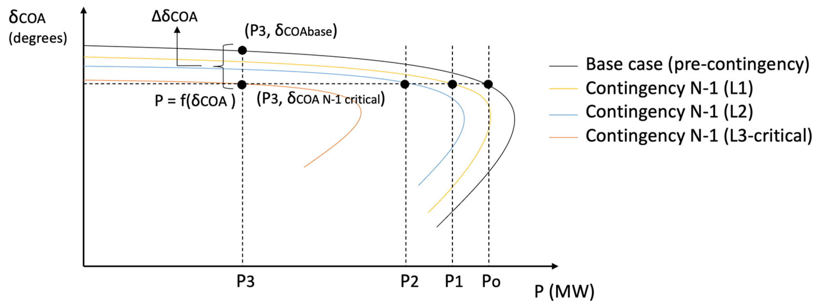
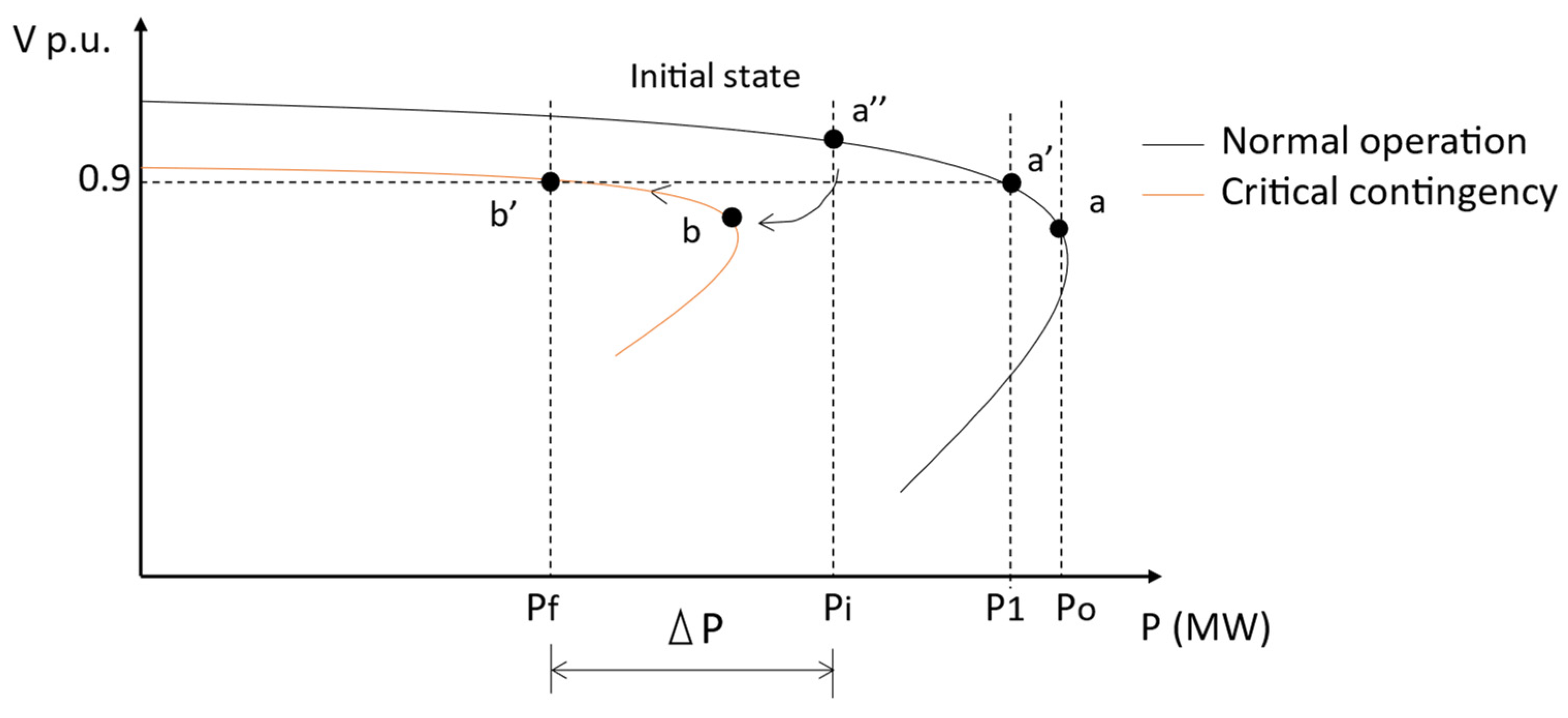
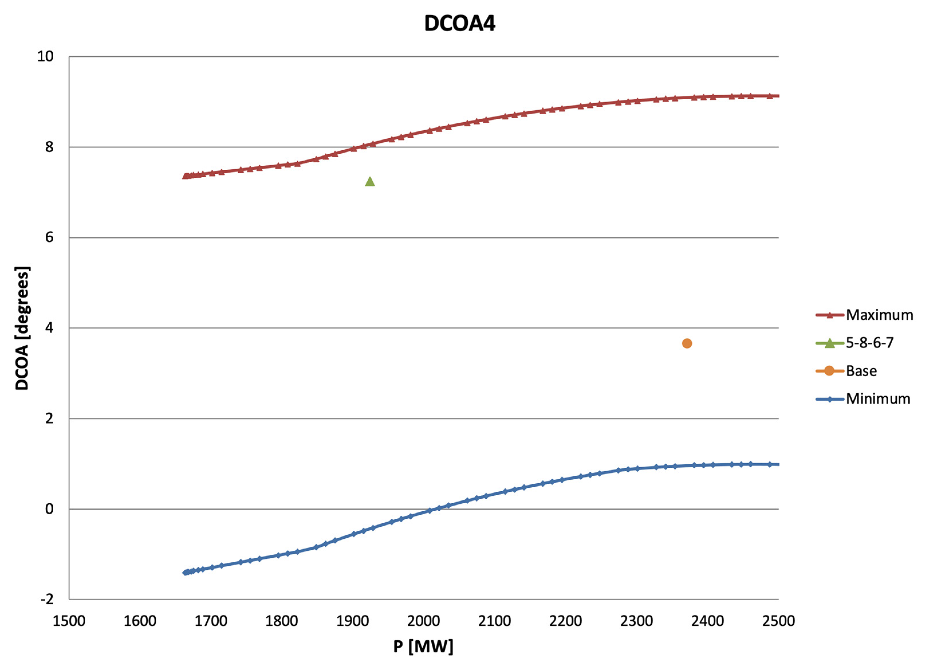
- a:
- Point of maximum power in bus i before non-convergence for the base case.
- a’:
- Safe operating point for the base case.
- a”:
- Safe operating point for the base case. It is the initial condition.
- b:
- Minimum voltage point found for bus i after carrying out the critical contingency from point a’’.
- b’:
- Safe operating point for critical contingency.
6. Simulation
7. Results
8. Conclusions
Author Contributions
Funding
Data Availability Statement
Acknowledgments
Conflicts of Interest
References
- Hatziargyriou, N.; Milanovic, J.; Rahmann, C.; Ajjarapu, V.; Canizares, C.; Erlich, I.; Hill, D.; Hiskens, I.; Kamwa, I.; Pal, B.; et al. Definition and Classification of Power System Stability—Revisited & Extended. In IEEE Transactions on Power Systems; IEEE: Piscataway, NJ, USA, 2021; Volume 36, pp. 3271–3281. [Google Scholar] [CrossRef]
- Eremia, M.; Shahidehpour, M. Background of Power System Stability, the Handbook of Electrical Power System Dynamics: Modeling, Stability, and Control; Wiley-IEEE Press: Hoboken, NJ, USA, 2013. [Google Scholar]
- Eremia, M.; Shahidehpour, M. Major Grid Blackouts: Analysis, Classification, and Prevention, the Handbook of Electrical Power System Dynamics: Modeling, Stability, and Control; Wiley-IEEE Press: Hoboken, NJ, USA, 2013. [Google Scholar]
- Van Cutsem, T.; Vournas, C. Voltage Stability of Electric Power Systems; Springer: Berlin/Heidelberg, Germany, 2008. [Google Scholar]
- Taylor, C.W.; Erickson, D.C.; Martin, K.E.; Wilson, R.E.; Venkatasubramanian, V. WACS—Wide-area stability and voltage control system: R&D and online demonstration. In Proceedings of the IEEE; IEEE: Piscataway, NJ, USA, 2005; Volume 93, pp. 892–906. [Google Scholar] [CrossRef]
- Sherwood, M.; Ajjarapu, V.; Leonardi, P.B. Real-Time Security Assessment of Angle Stability and Voltage Stability Using Synchrophasors Final Project Report Project Team Vaithianathan ‘Mani’ Venkatasubramanian (project leader). 2010. Available online: http://www.pserc.org (accessed on 1 July 2022).
- Su, H.-Y.; Liu, C.-W. Estimating the Voltage Stability Margin Using PMU Measurements. IEEE Trans. Power Syst. 2015, 31, 1–9. [Google Scholar] [CrossRef]
- Phadke, A.G.; Thorp, J.S. Synchronized Phasor Measurements and Their Applications; Springer: Berlin/Heidelberg, Germany, 2008. [Google Scholar]
- Pourbagher, R.; Derakhshandeh, S.Y.; Golshan, M.E.H. A novel method for online voltage stability assessment based on PMU measurements and Thevenin equivalent. IET Gener. Transm. Distrib. 2022, 16, 1780–1794. [Google Scholar] [CrossRef]
- Peng, L.; Li, Y.; Mili, L.; Tang, Y.; Xu, Y.; Zhao, B.; Li, J. A Real-Time Enhanced Thevenin Equivalent Parameter Estimation Method for PLL Synchronization Stability Control in VSC. IEEE Trans. Power Deliv. 2022, 37, 2650–2660. [Google Scholar] [CrossRef]
- O’Brien, J.; Deronja, A.; Apostolov, A.; Arana, A.; Begovic, M.; Brahma, S.; Brunello, G.; Calero, F.; Faulk, H.; Hu, Y.; et al. Use of synchrophasor measurements in protective relaying applications. In Proceedings of the 2014 67th Annual Conference for Protective Relay Engineers, College Station, TX, USA, 31 March–3 April 2014. [Google Scholar]
- Sahu, P.; Verma, M.K. Online monitoring of voltage stability margin using PMU measurements. Int. J. Electr. Comput. Eng. 2020, 10, 1156–1168. [Google Scholar] [CrossRef]
- Paramo, G.; Bretas, A.; Meyn, S. Research Trends and Applications of PMUs. Energies 2022, 15, 5329. [Google Scholar] [CrossRef]
- Ashwin, N.; Sreedevi, J.; Dixit, P.; Meera, K.S. Voltage stability of power system using pv curve and pmu data. Int. J. Recent Technol. Eng. 2019, 8, 7654–7659. [Google Scholar] [CrossRef]
- Wang, X.; Chiang, H. Analytical Studies of Quasi Steady-State Model in Power System Long-Term Stability Analysis. IEEE Trans. Circuits Syst. I Regul. Pap. 2014, 61, 943–956. [Google Scholar] [CrossRef]
- Dobson, I.; Parashar, M. A cutset area concept for phasor monitoring. In Proceedings of the IEEE PES General Meeting, Minneapolis, MN, USA, 25–29 July 2010. [Google Scholar]
- Dobson, I.; Parashar, M.; Carter, C. Combining Phasor Measurements to Monitor Cutset Angles. In Proceedings of the 2010 43rd Hawaii International Conference on System Sciences, Honolulu, HI, USA, 5–8 January 2010; IEEE: Piscataway, NJ, USA, 2010. [Google Scholar]
- Lopez, G.J.; Gonzalez, J.W.; Leon, R.A.; Sanchez, H.M.; Isaac, I.A.; Cardona, H.A. Proposals based on cutset area and cutset angles and possibilities for PMU deployment. In Proceedings of the 2012 IEEE Power and Energy Society General Meeting, San Diego, CA, USA, 22–26 July 2012; pp. 1–6. [Google Scholar] [CrossRef]
- López, G.; González, J.; Díez, A.; Isaac, I.; Cardona, H.A.; Leon, R.A. Contingency Analysis Model of Electrical Power Systems Based on Central Angles from PMUs. Adv. Mat. Res. 2013, 772, 664–672. [Google Scholar] [CrossRef]
- Darvishi, A.; Dobson, I. Threshold-Based Monitoring of Multiple Outages with PMU Measurements of Area Angle. IEEE Trans. Power Syst. 2016, 31, 2116–2124. [Google Scholar] [CrossRef] [Green Version]
- Sherwood, M.; Hu, D.; Venkatasubramanian, V.M. Real-time detection of angle instability using synchrophasors and action principle. In Proceedings of the 2007 iREP Symposium-Bulk Power System Dynamics and Control-VII. Revitalizing Operational Reliability, Charleston, SC, USA, 19–24 August 2007; IEEE: Piscataway, NJ, USA, 2007. [Google Scholar] [CrossRef]
- Feng, K.; Zhang, Y.; Liu, Z.; Li, T.; Ma, H. A wide area information based online recognition of coherent generators in power system. Dianwang Jishu/Power Syst. Technol. 2014, 38, 2082–2086. [Google Scholar] [CrossRef]
- Matevosyan, J.; Badrzadeh, B.; Prevost, T.; Quitmann, E.; Ramasubramanian, D.; Urdal, H.; Achilles, S.; MacDowell, J.; Huang, S.H.; Vital, V.; et al. Grid-forming inverters: Are they the key for high renewable penetration? In IEEE Power and Energy Magazine; IEEE: Piscataway, NJ, USA, 2019; Volume 17, pp. 89–98. [Google Scholar] [CrossRef]
- Denis, G.; Prevost, T. MIGRATE D3.6: Requirement guidelines for operating a grid with 100% power electronic devices. Migrate Proj. 2019, 10. [Google Scholar] [CrossRef]
- Haldar, A.; Khatua, R.; Malkhandi, A.; Senroy, N.; Mishra, S. Delay Based Virtual Inertia Emulation for a Grid Forming System. In 2022 IEEE Power and Energy Conference at Illinois (PECI); IEEE: Piscataway, NJ, USA, 2022; pp. 1–6. [Google Scholar] [CrossRef]
- Qi, Y.; Deng, H.; Liu, X.; Tang, Y. Synthetic Inertia Control of Grid-Connected Inverter Considering the Synchronization Dynamics. IEEE Trans. Power Electron. 2022, 37, 1411–1421. [Google Scholar] [CrossRef]
- Thilakarathne, C.; Meegahapola, L.; Fernando, N. Real-time voltage stability assessment using phasor measurement units: Influence of synchrophasor estimation algorithms. Int. J. Electr. Power Energy Syst. 2020, 119, 105933. [Google Scholar] [CrossRef]
- Lee, Y.; Han, S. Real-time voltage stability assessment method for the Korean power system based on estimation of Thévenin equivalent impedance. Appl. Sci. 2019, 9, 1671. [Google Scholar] [CrossRef]
- Kiseng, S.M.; Muriithi, C.M.; Nyakoe, G.N. Under voltage load shedding using hybrid ABC-PSO algorithm for voltage stability enhancement. Heliyon 2021, 7, e08138. [Google Scholar] [CrossRef] [PubMed]
- Ajjarapu, V.; Christy, C. The continuation power flow: A tool for steady state voltage stability analysis. In IEEE Transactions on Power Systems; IEEE: Piscataway, NJ, USA, 1992; Volume 7, pp. 416–423. [Google Scholar] [CrossRef]
- Lopez, G.J.; Gonzalez, J.W.; Escobar, D.A.; Leon, R.A.; Isaac, I.A.; Cardona, H.A. Network characterization based on central angles and PMU deployment. In Proceedings of the 2012 IEEE Power and Energy Society General Meeting, San Diego, CA, USA, 22–26 July 2012; IEEE: Piscataway, NJ, USA, 2012; pp. 1–6. [Google Scholar] [CrossRef]
- Darvishi, A.; Dobson, I. Area angle can monitor cascading outages with synchrophasors. In Proceedings of the 2015 IEEE Power & Energy Society Innovative Smart Grid Technologies Conference, Washington, DC, USA, 18–20 February 2015; IEEE: Piscataway, NJ, USA, 2015. [Google Scholar] [CrossRef] [Green Version]
- Dobson, I. Voltages Across an Area of a Network. In IEEE Transactions on Power Systems—IEEE TRANS POWER SYST; IEEE: Piscataway, NJ, USA, 2012; Volume 27, pp. 993–1002. [Google Scholar] [CrossRef]
- Aljarrai, K.; Sherwali, H. Using WACS Algorithm based on Center of Angle (COA) Technique in Assessing the Stability of the Libyan Grid. In Proceedings of the 2021 IEEE 1st International Maghreb Meeting of the Conference on Sciences and Techniques of Automatic Control and Computer Engineering MI-STA, Tripoli, Libya, 25–27 May 2021; IEEE: Piscataway, NJ, USA, 2021. [Google Scholar] [CrossRef]
- Real-Time Security Assessment of Angle Stability Using Synchrophasors Final Project Report PSERC. 2010. Available online: http://www.pserc.org (accessed on 1 July 2022).
- Lauby, M.G.; Kundur, P.; Balu, N.J. Power System Stability and Control; McGraw-Hill: New York, NY, USA, 1994. [Google Scholar]
- Chow, J.; Chakrabortty, A.; Arcak, M.; Bhargava, B.; Salazar, A. Synchronized Phasor Data Based Energy Function Analysis of Dominant Power Transfer Paths in Large Power Systems. In IEEE Transactions on Power Systems; IEEE: Piscataway, NJ, USA, 2007; Volume 22, pp. 727–734. [Google Scholar] [CrossRef]


| Area | Busbars | Generation [MW] | Load [MW] |
|---|---|---|---|
| Area 1 | 1, 2, 3, 18, 25, 30, 37 | 790 | 704 |
| Area 2 | 17, 26, 27, 28, 29, 38 | 830 | 909.5 |
| Area 3 | 4, 5, 6, 7, 8, 9, 10, 11, 12, 13, 31, 32, 39 | 2170.8 | 2376.5 |
| Area 4 | 14, 15, 16, 19, 20, 21, 22, 23, 24, 33, 34, 35, 36 | 2350 | 2107 |
| Area | Load [MW] | DCOA1 [°] | DCOA3 [°] | DCOA4 [°] | DCOA3 [°] |
|---|---|---|---|---|---|
| 1 | 1048.19 | −3.70 | 3.82 | −2.38 | 2.44 |
| 2 | 1008.86 | −1.63 | 4.60 | −4.70 | 3.46 |
| 3 | 2606.78 | −1.86 | 6.11 | −4.88 | 3.47 |
| 4 | 2157.88 | −1.38 | 6.37 | −5.43 | 3.36 |
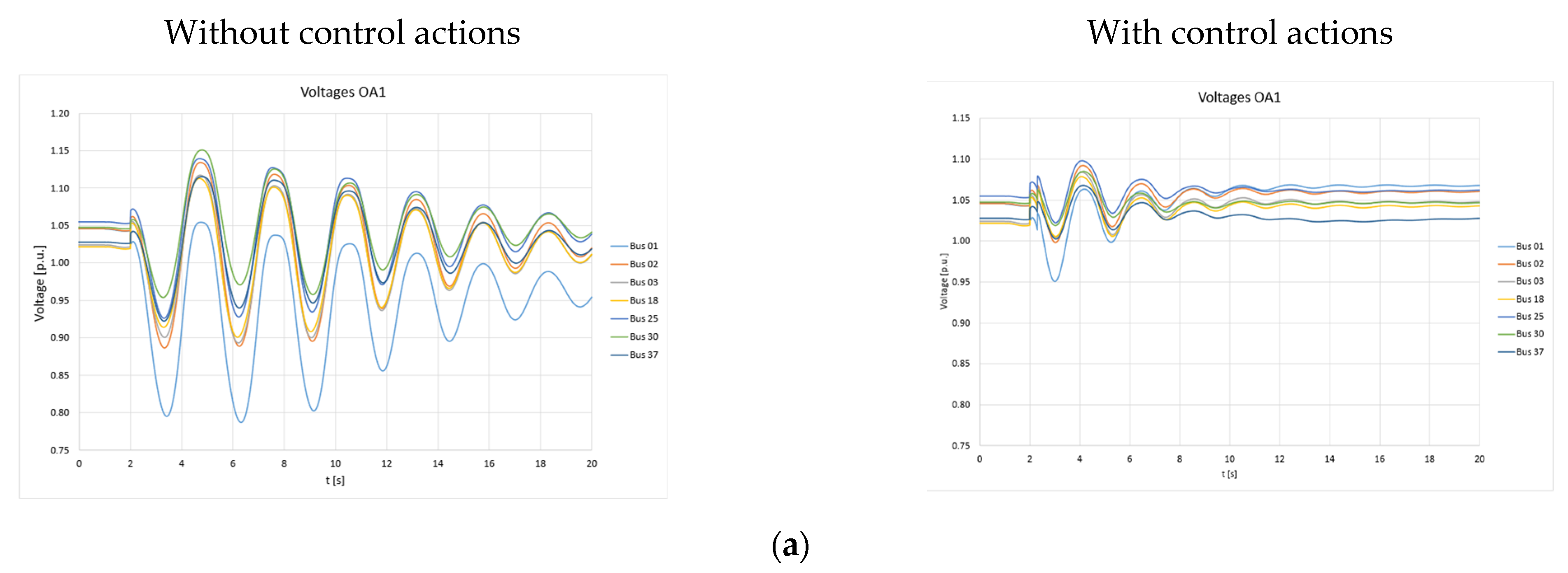
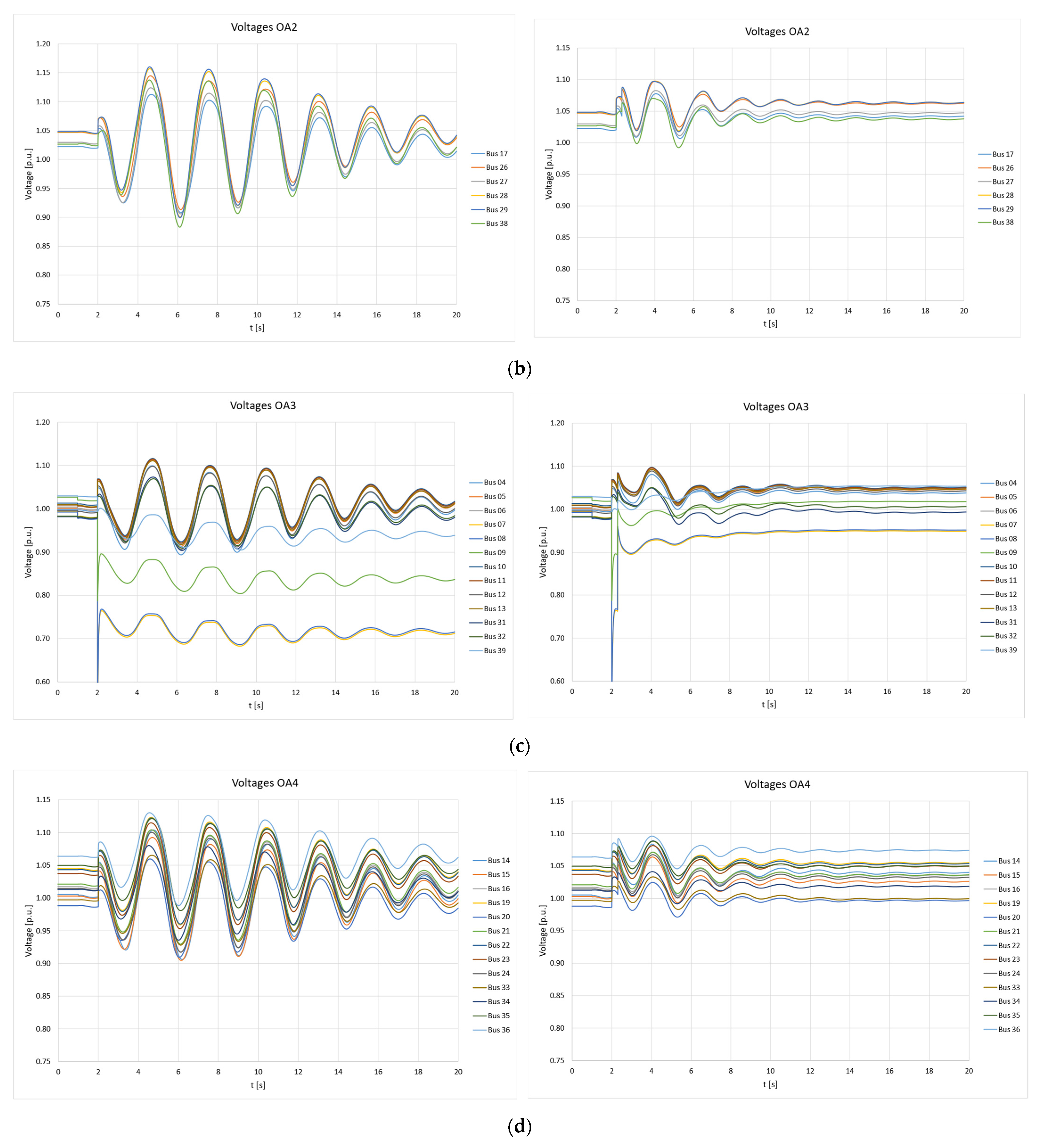
| Most Affected Voltage Bus in OA | Maximum Voltage Deviation w/o COA Method | Maximum Voltage Deviation with COA Method | Minimum Voltage Deviation w/o COA Method | Minimum Voltage Deviation with COA Method | Voltage Stabilization Time w/o COA Method [s] | Voltage Stabilization Time w/o COA Method [s] |
|---|---|---|---|---|---|---|
| 1 | 1.150 | 1.098 | 0.787 | 0.951 | 17 | - |
| 2 | 1.157 | 1.096 | 0.883 | 0.992 | 16 | - |
| 3 | 1.111 | 1.092 | 0.686 | 0.897 | >20 | 4 |
| 4 | 1.130 | 1.095 | 0.911 | 0.971 | 16 | - |
Publisher’s Note: MDPI stays neutral with regard to jurisdictional claims in published maps and institutional affiliations. |
© 2022 by the authors. Licensee MDPI, Basel, Switzerland. This article is an open access article distributed under the terms and conditions of the Creative Commons Attribution (CC BY) license (https://creativecommons.org/licenses/by/4.0/).
Share and Cite
Lopez, G.J.; González, J.W.; Isaac, I.A.; Cardona, H.A.; Vasco, O.H. Voltage Stability Control Based on Angular Indexes from Stationary Analysis. Energies 2022, 15, 7255. https://doi.org/10.3390/en15197255
Lopez GJ, González JW, Isaac IA, Cardona HA, Vasco OH. Voltage Stability Control Based on Angular Indexes from Stationary Analysis. Energies. 2022; 15(19):7255. https://doi.org/10.3390/en15197255
Chicago/Turabian StyleLopez, Gabriel J., Jorge W. González, Idi A. Isaac, Hugo A. Cardona, and Oscar H. Vasco. 2022. "Voltage Stability Control Based on Angular Indexes from Stationary Analysis" Energies 15, no. 19: 7255. https://doi.org/10.3390/en15197255