Evaluating Regional Carbon Inequality and Its Dependence with Carbon Efficiency: Implications for Carbon Neutrality

Abstract

This paper proposes a novel regional carbon emission inequality (RCI) index based on a special kind of general distribution. Using the proposed RCI index and based on China’s county-level panel data over the time span of 1997–2017, the regional carbon emission inequality of China is evaluated at intra-provincial, sub-national, and national levels. Based on that, the dependence between regional carbon inequality and carbon efficiency is studied by using copula functions and nonlinear dependence measures. The empirical results show that: (1) Shanghai, Tianjin, and Inner Mongolia have the worst carbon inequalities; while Hainan, Qinghai, and Jiangxi are the three most carbon-equal provinces; (2) there is a divergence phenomenon in RCI values of municipalities over the past decade; (3) from the national-level perspective, the inter-provincial carbon emission inequality is much greater than that at the intra-provincial level; (4) from the sub-national-level perspective, the east region has the highest RCI value, followed by the northeast, west, and the central regions; (5) there is a so-called "efficiency-equality (E-E) trade-off" in each provincial administrative unit, meaning that the higher carbon efficiency generally comes with higher carbon inequality, i.e., carbon efficiency comes at a price of carbon inequality; and (6) by re-grouping provincial units via the efficiency-equality cost and industrial structure, respectively, both carbon equality and carbon efficiency can be achieved in some regions simultaneously, thereby getting out of the “E-E trade-off” dilemma. The empirical evidence may provide valuable insight regarding the topic of “equality and efficiency” in environmental economics, and offer policy implications for regional economic planning and coordination.

1. Introduction

To date, more and more countries have actively participated in climate change intensification actions such as carbon neutrality. For example, in 2017, 29 countries signed the “Carbon Neutrality Alliance Statement”, promising to achieve zero carbon emissions in the mid-21st century; at the UN summit in September 2019, 66 countries pledged to achieve carbon neutrality goals and formed a climate ambition Alliance; in May 2020, 449 cities around the world participated in the zero-carbon race proposed by UN climate experts; as of February 2021, 127 countries have committed to carbon neutrality by the middle of the 21st century (Zhao et al., 2022) [1]. At present, countries such as Bhutan and Suriname have achieved carbon neutrality goals, and countries such as the United Kingdom, Sweden, France, and New Zealand have written carbon neutrality into their laws. In November 2020, 19 countries that account for 50% of global greenhouse gas emissions submitted long-term low-emission development strategies (LTS) to the United Nations Framework Convention on Climate Change (UNFCCC), of which 11 countries’ LTS included carbon neutrality goals and committed to achieve carbon neutrality (Demirkhanyan, 2020) [2].

At the general debate of the 75 th United Nations General Assembly in September 2020, China pledged to “increase the nationally determined contribution, adopt more powerful policies and measures, strive to peak carbon dioxide emissions before 2030, and strive to achieve a peak in carbon dioxide emissions by 2060 to achieve carbon neutrality.” (Dong et al., 2021) [3]. This commitment brings new opportunities as well as new challenges to China’s economic development under the “new normal.”

In fact, carbon neutrality is providing favorable foundations and conditions for systematical change in economies around the world. Carbon neutrality provides opportunities for international cooperation in related fields, such as guiding international green capital flow, talent employment, green industry and renewable energy venture capital and financing, etc. (Tian et al., 2022) [4]. Countries are actively developing green finance to promote economic recovery after the COVID-19 epidemic; countries have introduced incentives to provide financial support and tax incentives to enterprises, increase investment in technology research and development and industrialization, develop green industry funds, and guide social funds to invest, to promote the comprehensive transformation and upgrading of industries oriented to sustainable development (Vaka et al., 2020) [5]. The development of green finance has become the consensus of all countries, and the green finance market has gradually matured (Sadiq et al., 2021) [6].

Despite the opportunity, however, it must be admitted that achieving carbon neutrality rapidly is still challenging for lots of economies, especially the world’s second-largest one (Liu et al., 2022) [7]. In fact, there is a precondition for carbon neutrality, that is, carbon peaking (Zhao et al., 2022) [8]. The time and level of carbon peaking directly affect the time and difficulty of achieving carbon neutrality. The earlier the peak time, the less pressure to achieve carbon neutrality; the higher the peak, the more technological advance and social costs are required to achieve carbon neutrality (Zhang, 2021) [9]. Thus, in order to achieve carbon peaking as soon as possible and then achieve carbon neutrality, what the government, enterprises, and other economic entities can do is to realize the improvement of technical efficiency and carbon efficiency as soon as possible (Jia and Lin, 2021) [10].

Meanwhile, one of the possible risks in the process of carbon peaking and carbon neutrality is that regional economic inequality may increase (Liu et al., 2022) [7]. In terms of China, Shandong, Jiangsu, Hebei, Inner Mongolia, and Henan, which rank in the top 5 in China in terms of total carbon emissions, are facing greater pressures for carbon emission reduction and green and low-carbon transformation (Zhang et al., 2022) [11]. The existing carbon peak and carbon neutral paths and scenarios in large cities are difficult to adapt to the low-carbon development of small and medium-sized cities (Pan et al., 2022) [12]. With the comprehensive green transformation of economic and social development, the central and west regions will face many challenges, such as the decline of regional ecological environment carrying capacity, the weak competitiveness of resource-based enterprises, the lack of corporate innovation capabilities, the shortage of scientific and technological talents, and the lack of sound systems and mechanisms for green development. If these problems are not handled properly, there will be a “lose–lose” of resources and economic development in some regions (Liu et al., 2022; Pan et al., 2022) [7,12].

Therefore, in the current context, for China’s long-term goal of “achieving carbon neutrality”, its connotation is that China’s economic development must firstly achieve carbon peaking, which requires the reduction of regional carbon emission inequality and the improvement of carbon emission efficiency simultaneously (Chi et al., 2021; Liu et al., 2022) [7,13].

In the literature, lots of related topics have been discussed by researchers, such as carbon inequality, carbon efficiency, and their relationship with carbon neutrality, which lay a valuable basis for our study (see Section 2). Nevertheless, there are still some gaps in the existing study. First, whereas many studies have proposed the carbon inequality measures with respect to other variables, the research working on measuring the regional carbon inequality is scarce. As a matter of fact, most of the existing carbon inequality indexes proposed are “relative” measures rather than “absolute” measures. A relative measure means that it considers the relative inequality of carbon emissions with respect to other economic variables such as individual income or household wealth. Technically, this can be done by calculating the percentile of carbon emission corresponding to the percentile of a given economic variable. Examples of the relative inequality measures include Gini Index (Heil and Wodon, 1997; Teixido-Figueras et al., 2016) [14,15], Theil Index (Padilla and Duro, 2013) [16,17], and the Lorenz curve (Zhang et al., 2021) [18], etc. In contrast, to measure carbon inequality at the spatial level, one does not need to calculate any relative weight, but needs to characterize how asymmetrical the distribution of carbon emissions can be, spatially. This is a so-call “absolute” measure, because it is a “pure” measure of the inequality and asymmetry of carbon emission per se. Second, even though the dependence between many environmental variables has been studied, such as wind energy yield (Schindler and Jung, 2018) [19], heating energy consumption (Niemierko et al., 2019) [20], and the relationship between carbon emission and industrial production (Gozgor et al., 2020) [21], the research working on the dependence between regional carbon inequality and regional carbon efficiency is very few. Third, few of the existing literature discussed the possible policy for coordinating the “equality” and “efficiency” issues of carbon emission under the carbon neutrality background. Finally, in the literature, the economic dependence of carbon emission has been found in governmental expenditures, energy consumption (Fan et al., 2020) [22], energy inequality (Zhong et al., 2020) [23], and regional income inequality (Cui et al., 2021) [24]. Nevertheless, very few of the current works discussed the “trade-off” between carbon efficiency and carbon inequality. In welfare economics, efficiency and fairness (and a similar connotation, equality) and their relationship are important issues. However, efficiency and equality may not always be achieved simultaneously. Sometimes efficiency gains come at the cost of equality reductions. This is the so-called “trade-off.” For the environmental economic study, it would be of both academic and practical significance to investigate if the trade-off also exists in the relationship between carbon efficiency and carbon inequality.

To fill the current gaps, this paper applies contemporary statistical methodologies such as general distribution, copula function, and tail dependence measure. We contribute to the literature from the following four aspects. First, based on a kind of general distribution which includes both symmetrical and asymmetrical distributions as special cases, this paper proposes a novel regional carbon inequality index (RCI), which can be an ideal measure to evaluate the “pure” degree of carbon inequality at the spatial (regional) level. Different from the conventional carbon inequality evaluation tools which are “relative” measures, the proposed RCI index is a direct and “absolute” measure of the degree of inequality in regional carbon emission per se. Second, overall dependence and tail dependence between regional carbon inequality and regional carbon efficiency is investigated by using the copula functions and tail dependence measure, which may be an increment to the existing nonlinear dependence evidence in the environmental area (see Section 2 for detailed review). Third, by grouping and comparing the dependence between grouped and ungrouped results, possible implications for regional planning and coordination policies can be offered, which would be conducive to the carbon neutrality goal. Last but not least, our empirical results may provide valuable evidence for the topic of “efficiency and equality” in economics, as it addresses issues of resource allocation and economic efficiency. It is worth noting that the reason why we want to figure out the “pure” degree of carbon inequality at the spatial (regional) level is that excessive carbon emission inequality may imply an excessive concentration of economic resources in some regions, thereby leading to economic inefficiency. In this sense, discussing the “pure” degree of regional carbon inequality, i.e., investigating the “absolute” inequality rather than “relative” inequality, is the precondition to study the relationship between equality and efficiency from an environmental economic perspective.

The rest of this paper is organized as follows. Section 2 reviews the literature. Data and variables utilized in this paper are introduced in Section 3. In Section 4, we explain the statistical approachesadopted in the study. Section 5 displays the empirical results. Section 6 concludes the paper, offers policy implications, and points out possible future study directions.

2. Literature Review

2.1. Literature regarding Carbon Inequality

In the literature, carbon emission inequality and its possible causes are hotly debated topics. Fang et al. (2019) [25] utilize a multi-regional input-output model to explore the regional mismatch of economic benefits, air pollutants (primary PM2.5), and carbon emissions, as well as the environmental and economic inequality between urban and rural consumption. Wang et al. (2019) [26] estimate disparities in carbon intensity in China using a multi-scalar and multi-mechanism analysis. Pan et al. (2019) [27] propose a new indicator—the carbon Palma ratio, which provides a new perspective to inform the international community and the public of the distribution inequality of carbon emissions among individuals. Du et al. (2019) [28] use the Gini index and Theil index to examine carbon inequality in the transport sector in China and decompose the per capital carbon inequality using Kaya factors. Mushtaq et al. (2020) [29] aim to investigate the impact of income inequality and economic growth on carbon dioxide (CO₂) emission through the moderating role of innovation in China at national and regional levels. Using the Theil index and the logarithmic mean Divisia index decomposition approach, Fan et al. (2020) [22] integrate government expenditure into an analysis framework, investigating the driving factors of emission inequality and the status and changes of China’s CO₂ emission inequality from 2007 to 2015, attributing emission inequality to disparities in governmental expenditures, energy consumption, and other socioeconomic factors. Han et al. (2020) [30] compare the carbon emissions driven by final demand among countries in and outside the Belt and Road area from 1990 to 2015. Zhong et al. (2020) [23] focus on carbon and energy inequality between and within ten Latin American and Caribbean (LAC) countries. Cui et al. (2021) [24] analyze the relationship between carbon emission efficiency and the regional income inequality, and find that when the carbon emission reduction efficiency increases by one unit, the income inequality gap of 25 provinces increases by 0.0202 units; provinces with high carbon emission reduction efficiency increases by 0.107 units, and provinces with medium carbon emission reduction efficiency increases by 0.026 units. Using the provincial panel data of the Chinese residential sector from 2005 to 2017, Wang et al. (2021) [31] examine residential CO₂ emission inequality (carbon inequality) and its driving factors from the static and dynamic perspectives to provide empirical support for the formulation of emission reduction policies and the allocation of regional emission reduction quotas. Based on the provincial panel data and industrial enterprise panel data in China from 1998 to 2017, Zhang et al. (2021) [32] explore if China’s emission trading scheme (ETS) pilot policy brings the double dividends of green development efficiency and regional carbon equality by using the DID model and Malmquist-Luenberger (ML) index. For measuring carbon inequality, the most commonly used methods in the existing literature are the Gini Index (Heil and Wodon, 1997; Teixido-Figueras et al. 2016) [14,15], variation coefficient (Duro, 2012) [33], the Theil Index (Padilla and Duro, 2013) [16], multi-regional input–output (MRIO) method (Hubacek et al., 2017) [17], and the Lorenz curve (Zhang et al., 2021) [18]. It is worth noting that the above indexes are based on the carbon inequalities related to individual income and household consumption, which are relative measures. The study proposing an absolute measure of carbon inequality is scarce.

2.2. Literature Regarding Carbon Efficiency

Parallel to the above work, many studies in the literature also involve the measurement and cause analysis of carbon emission efficiency. On the ond hand, lots of the existing studies have used the latest statistics and optimization techniques to measure carbon emission efficiency. Zhang et al. (2018) [34] propose a modified data envelopment analysis (DEA) to analyze the carbon efficiency decomposition and potential material reduction for regional construction industries. Zhou et al. (2021) [35] evaluate the carbon dioxide emission from China’s regional construction industry by the three-stage DEA method, and evidence that climate change is an important starting point for promoting the high-quality development of China’s economy and the construction of ecological civilization, as well as an important area for participating in global governance and adhering to multilateralism. Based on China’s Jiangsu Province’s data, Tan and Wang (2021) [36] utilize the super-efficiency DEA model and the Tobit model to verify the main factors affecting regional ecological efficiency and find that the regional eco-efficiency in Jiangsu shows a trend of decreasing from south to north, with the obvious phenomenon of “club convergence”, with significant spatial correlation and agglomeration.

On the other hand, kinds of literature also look for the driving factors of carbon emission efficiency from the perspectives of industry or space. Liu et al. (2019) [37] propose a multi-region multi-sector decomposition and attribution approach to analyze the driving forces of ACI from both sectoral and regional perspectives, and the result shows that the ACI declined by 33% from 2000 to 2015. From the sectoral perspective, the decline can be mainly attributed to the significant energy efficiency improvement in six high energy-intensive industries. Regarding the spatial effect of carbon efficiency, Wang et al. (2021) [38] explore the spatial distribution of industrial resource allocation efficiency and carbon emissions using the panel data of 30 provinces from 2007 to 2016, which evidence that the improvement of industrial resource allocation can reduce carbon emissions on the national level and industrial resource allocation can significantly reduce carbon emissions in the east region. Similar research using spatial econometrics can be found in Zhang et al., 2021 [18], Yang et al., 2021 [39], and Ma et al., 2022 [40].

2.3. Literature Regarding Dependence under Carbon Neutrality Background

Scholars have also explored the possible relationship between inequality and the achievement of carbon neutrality goals and have drawn many instructive conclusions from their empirical evidence. Zhu et al. (2018) [41] examine the effects of urbanization and income inequality on CO₂ emissions in the BRICS (i.e., Brazil, Russia, India, China, and South Africa) economies during the period 1994–2013. Dahal et al. (2018) [42] use multilevel perspective (MLP) and renewable energy frameworks to examine the role of renewable energy policies in carbon neutrality in the Helsinki Metropolitan area and base the analysis on various policy documents and semi-structured interviews. Considering the short- and long-term impacts of income inequality on carbon emissions, as well as the heterogeneity of the emission distribution, Liu et al. (2019) [43] employ panel ARDL and quantile regression models to analyze the effect of income inequality on carbon emissions across US states. Mi et al. (2020) [44] apply an environmentally extended multiregional input–output approach to estimate household carbon footprints for 12 different income groups of China’s 30 regions. Han et al. (2020) [30] compare the carbon emissions driven by final demand among countries in and outside the Belt and Road area from 1990 to 2015. The relationship among income inequality, renewable energy technological innovation (RETI), and CO emissions has not received sufficient attention in the current literature. Based on Chinese provincial panel data from 2000 to 2015, Bai et al. (2020) [45] adopt a panel fixed effect regression model and a panel threshold model to perform an analysis of the nonlinear relationship among these factors. Tan et al. (2021) [46] employ a nonlinear panel autoregressive distributed lag (ARDL) model, and find that reduction in income inequality is necessary to increase carbon neutrality potential.

Regarding the asymmetric features and non-linear dependence among environmental and economic variables, various statistical methods are utilized in the literature, such as general distributions, asymmetric distributions, dynamic time series models, and nonlinear dependence measure. Deng and Zhang (2018) [47] fit a generalized extreme value (GEV) distribution to exceedances over a station-specific extreme smog level of hourly PM2.5 data from 2014 to 2016 obtained from monitoring stations across China. Deng et al. (2020) [48] develop a dynamic model of conditional exponentiated Weibull distribution modeling and analysis of regional smog extremes and provide useful information for the central/local government to conduct coordinated PM_2.5 control and treatment. A variety of studies apply nonlinear dependence (for example, copula) to examine co-movement between two or more inter-connected variables of interest in a range of research areas, such as energy, environment, and forestry. Schindler and Jung (2018) [19] use the mixed Burr-Generalized extreme value distribution (BGEV) and Gaussian copulas in a two-step procedure to estimate the directional wind energy yield at 100 m above ground level in Germany. Niemierko et al. (2019) [20] develop a D-vine copula-based quantile regression to predict quantiles of heating energy consumption and reveal cyclical rebound effect dependent on retrofit level. Gozgor et al. (2020) [21] employ the time-varying Markov-switching copula models to examine the inter-dependence relations between CO₂ emissions and the industrial production index as a measure of business cycles at the monthly frequency in the United States. As an inheritance of methods commonly used in the related literature, this paper also uses general distributions and dependence measures in our study. Based on that, a novel regional carbon inequality can be proposed and the dependence between regional carbon inequality and regional carbon efficiency can be studied, which is an increment to the literature.

3. Data and Variables

3.1. Sample and Data Sources

There are two research purposes of this study: (1) to propose a “pure” measure of regional carbon inequality (RCI); and (2) to investigate the dependence between regional carbon inequality and regional carbon efficiency. The output of the first step, i.e., the regional carbon inequality estimation, is the input of our second step. Consequently, policy implications for carbon neutralization can be offered based on the empirical results. Therefore, this study needs to use kinds of panel data: (1) regional carbon emission; and (2) regional carbon emission efficiency.

The carbon emission data used in this paper is mainly the county-level annual data of China from 1997 to 2017, which is computed and offered by Chen et al., (2020) [49] and can be downloaded from the Carbon Emission Accounts & Datasets (CEADs) (https://www.ceads.net/user/index.php?id=1057&lang=en, accessed on 12 November 2020). This dataset is a panel data that includes 2735 counties in 325 cities of 30 provinces in China over 21 years. Taiwan, Hong Kong, Macao, and Tibet are excluded due to the lack of CO₂ emission observations. In addition, we estimate the national-level RCI in Section 5.1.2 using the provincial-level carbon emission panel data, so as to investigate the inter-provincial carbon inequality. We note that this is the only place in this paper that uses the provincial panel dataset. Except for the national-level RCI estimation, all other research in this paper are based on the county-level panel data which is introduced above. The provincial-level carbon emission panel data is generated and offered by Shan et al. (2016) [50], Shan et al. (2018) [51], Shan et al. (2020) [52], and Guan et al. (2021) [53], which can be downloaded from https://www.ceads.net/data/province/, (accessed on 21 October 2021). It contains 30 provinces in China over 23 years from 1997 to 2019. All carbon emission data are measured in metric ton (mt).

The carbon emission efficiency data used in this paper is the one generated and offered by Ning et al. (2021) [54] using the super-efficiency SBM model. This dataset includes the carbon emission efficiency of 30 provincial-level administrative regions in China (excluding Taiwan, Hong Kong, Macao, and Tibet) from 2007 to 2016, which is reported in

Table A1. The carbon emission efficiency data of 30 provincial-level administrative regions in China (excluding Taiwan, Hong Kong, Macao, and Tibet) from 2007 to 2016, which is given by Ning et al. (2021) [54].

Province	2008	2009	2010	2011	2012	2013	2014	2015	2016
Beijing	1.140	1.147	1.159	1.217	1.19	1.201	1.199	1.199	1.216
Tianjin	0.658	0.665	0.662	0.658	0.672	0.736	0.71	0.741	0.808
Hebei	0.386	0.376	0.381	0.375	0.377	0.365	0.362	0.361	0.364
Shanxi	0.347	0.325	0.327	0.327	0.326	0.319	0.298	0.299	0.297
Inner Mongolia	0.353	0.366	0.373	0.368	0.362	0.375	0.366	0.371	0.376
Liaoning	0.42	0.42	0.427	0.425	0.428	0.428	0.418	0.421	0.404
Jilin	0.371	0.376	0.38	0.381	0.4	0.398	0.394	0.4	0.408
Heilongjiang	0.466	0.456	0.456	0.45	0.449	0.443	0.434	0.421	0.421
Shanghai	1.066	1.059	1.062	1.073	1.085	1.026	1.035	1.042	1.052
Jiangsu	0.617	0.619	0.618	0.602	0.616	0.603	0.613	0.619	0.627
Zhejiang	0.638	0.625	0.628	0.605	0.621	0.603	0.608	0.607	0.611
Anhui	0.419	0.416	0.427	0.422	0.427	0.409	0.407	0.404	0.407
Fujian	0.594	0.575	0.581	0.545	0.561	0.549	0.539	0.544	0.559
Jiangxi	0.492	0.49	0.488	0.475	0.488	0.468	0.47	0.467	0.473
Shandong	0.474	0.473	0.472	0.489	0.494	0.485	0.484	0.479	0.48
Henan	0.384	0.378	0.394	0.382	0.39	0.373	0.367	0.365	0.37
Hubei	0.418	0.42	0.422	0.416	0.422	0.438	0.438	0.44	0.441
Hunan	0.448	0.447	0.446	0.435	0.445	0.453	0.453	0.453	0.455
Guangdong	1.101	1.091	1.088	1.081	1.07	1.056	1.04	1.033	1.027
Guangxi	0.455	0.442	0.421	0.396	0.397	0.381	0.378	0.379	0.373
Hainan	0.557	0.534	0.537	0.483	0.463	0.43	0.41	0.395	0.396
Chongqing	0.445	0.451	0.464	0.467	0.489	0.493	0.494	0.502	0.503
Sichuan	0.419	0.415	0.423	0.435	0.448	0.445	0.445	0.454	0.464
Guizhou	0.286	0.292	0.295	0.309	0.311	0.3	0.293	0.287	0.284
Yunnan	0.329	0.326	0.321	0.314	0.314	0.313	0.304	0.304	1.015
Shaanxi	0.389	0.387	0.391	0.389	0.392	0.381	0.377	0.395	0.38
Gansu	0.335	0.337	0.333	0.328	0.335	0.327	0.321	0.318	0.319
Qinghai	0.283	0.277	0.283	0.278	0.272	0.257	0.247	0.238	0.233
Ningxia	0.255	0.245	0.244	0.237	0.233	0.235	0.226	0.214	0.209
Xinjiang	0.357	0.341	0.335	0.324	0.312	0.295	0.283	0.273	0.266

in Appendix A.

According to the computation results in Ning et al. (2021) [54] (see Table A1 in Appendix A), the distribution of carbon emission efficiency among provinces in China is highly uneven. Beijing, Shanghai, and Guangdong are all at an effective level, while other provinces are not at an effective level. There are as many as 24 provinces with ineffective carbon emission efficiency, among which the three provinces with the lowest carbon emission efficiency are all located in the southwest of China, namely Ningxia, Qinghai, and Guizhou, and the lowest is Ningxia. The carbon emission efficiency of Yunnan province fluctuates the most during the sample periods.

Table 1. The descriptive statistics of the county-level annual carbon emission data.

Year	Obs	Mean	S.D.	Skewness	Kurtosis	Min	Max	J-B Stat	J-B p-Value
1997	2735	1.132	1.292	5.469	72.95	0.000	25.75	571,188.85	0
1998	2735	0.998	1.179	6.497	94.76	0.000	25.13	978,850.97	0
1999	2735	1.094	1.259	6.595	99.77	0.000	27.08	1,087,000.49	0
2000	2735	1.154	1.330	6.715	102.1	0.000	28.69	1,139,495.23	0
2001	2735	1.162	1.305	6.229	91.17	0.000	27.17	903,685.42	0
2002	2735	1.257	1.416	6.330	92.59	0.000	29.49	932,928.62	0
2003	2735	1.481	1.660	6.073	85.65	0.000	33.58	795,299.82	0
2004	2735	1.650	1.839	5.861	80.87	0.000	36.70	706,645.71	0
2005	2735	1.965	2.153	5.287	68.35	0.000	41.31	499,366.95	0
2006	2735	2.208	2.424	5.254	67.85	0.000	46.82	491,890.47	0
2007	2735	2.362	2.568	4.903	59.43	0.000	47.52	373,815.41	0
2008	2735	2.531	2.719	4.637	53.49	0.000	48.77	300,317.69	0
2009	2735	2.729	2.922	4.748	56.04	0.000	53.48	330,880.89	0
2010	2735	2.988	3.156	4.554	51.67	0.000	56.43	7,279,382.16	0
2011	2735	3.335	3.398	3.949	38.38	0.000	54.14	149,786.90	0
2012	2735	3.403	3.462	3.998	39.11	0.000	55.56	155,843.31	0
2013	2735	3.422	3.369	3.689	32.83	0.000	49.25	107,608.38	0
2014	2735	3.494	3.430	3.594	31.11	0.000	49.42	95,951.52	0
2015	2735	3.302	3.257	3.468	28.63	0.000	45.05	80,345.16	0
2016	2735	3.404	3.360	3.428	27.92	0.000	46.08	76,117.43	0
2017	2735	3.467	3.392	3.255	24.74	0.000	44.03	58,696.73	0

reports the descriptive statistics for the county-level carbon emission data by year. The mean and standard deviation of carbon emission basically increase over time. The maximum value of carbon emission increased year by year from 1997 to 2012, and decreased year by year from 2012 to 2017. For each year’s carbon emission data, the skewness is greater than 0, and the kurtosis is greater than 3. Both skewness and kurtosis increased year by year from 1997 to 2000 and decreased year by year from 2000 to 2017. These facts strongly imply that the annual carbon emission is highly asymmetrically distributed. Besides, the Jarque-Bera (J-B) tests (Jarque and Bera, 1987) [55] are conducted for the carbon emission data annually (see Table 1). All the resulting J-B statistics are larger than 50,000 with p-values equal to 0, which strongly reject all null hypotheses of normality at the 0.01 level. The J-B testing result means that the carbon emission may not be normally and symmetrically distributed, and thus one has to utilize a more general and flexible distribution for its fitting. In this paper, we utilize the exponential generalized beta of the second kind (EGB2) distribution to fit the carbon emission data as this distribution can perfectly capture the abnormal and asymmetric features of carbon emission (see Section 4.1) and is of great economic interpretability in measuring carbon inequality (see Section 4.1.2).

Table 2. The descriptive statistics of the annual carbon emission efficiency data.

Year	Obs	Mean	S.D.	Skewness	Kurtosis	Min	Max	J-B Stat	J-B p-Value
2007	30	0.499	0.229	1.738	5.241	0.251	1.126	21.38	$2.274\times {10}^{-5}$
2008	30	0.497	0.229	1.805	5.432	0.255	1.140	23.68	$7.204\times {10}^{-6}$
2009	30	0.492	0.230	1.820	5.498	0.245	1.147	24.36	$5.121\times {10}^{-6}$
2010	30	0.495	0.230	1.827	5.543	0.244	1.159	24.77	$4.180\times {10}^{-6}$
2011	30	0.490	0.236	1.962	6.056	0.237	1.217	30.93	$1.924\times {10}^{-7}$
2012	30	0.493	0.235	1.863	5.707	0.233	1.190	26.51	$1.755\times {10}^{-6}$
2013	30	0.486	0.233	1.827	5.624	0.235	1.201	25.29	$3.218\times {10}^{-6}$
2014	30	0.480	0.235	1.803	5.584	0.226	1.199	24.60	$4.553\times {10}^{-6}$
2015	30	0.481	0.237	1.744	5.391	0.214	1.199	22.35	$1.400\times {10}^{-5}$
2016	30	0.508	0.259	1.427	4.037	0.209	1.216	11.52	$3.145\times {10}^{-3}$

reports the descriptive statistics for the annual carbon emission efficiency data. As shown, the mean, variance, annual minimum, and annual maximum of carbon emission efficiency basically do not change with time. The Skewness and kurtosis are greater than 0 and 3 each year, respectively, indicating that the carbon emission efficiency data is highly asymmetric. J-B tests are conducted by year as well, and all the resulting J-B statistics are larger than 10 with p-values less than ${10}^{-3}$, suggesting that all the null hypotheses of normality are rejected at 0.01 level and the carbon emission efficiency is not normally distributed.

In Section 5.2 and Section 5.3, we study the dependence between regional carbon inequality and carbon emission efficiency. It is worth noting that the carbon emission efficiency data is calculated by the super-efficiency method by Ning et al., (2021) [54], and the regional carbon inequality is measured using the RCI index proposed in this paper (see Section 4.1.2).

Regarding our proposed variable and the resulting annual RCI values,

Table 3. The descriptive statistics of the intra-provincial carbon inequality measure.

Year	Obs	Mean	S.D.	Skewness	Kurtosis	Min	Max	J-B Stat	J-B p-Value
1997	30	17.63	76.84	5.092	27.27	0.071	421.7	866.1	0
1998	30	15.31	66.18	5.065	27.08	0.057	362.7	853.0	0
1999	30	18.29	81.59	5.111	27.41	0.060	447.8	875.3	0
2000	30	20.25	88.29	5.080	27.19	3.383	484.1	860.3	0
2001	30	16.61	70.28	5.043	26.91	−0.126	384.9	842.0	0
2002	30	22.91	99.50	5.086	27.23	−0.201	545.9	863.0	0
2003	30	35.88	155.5	5.078	27.17	−0.525	852.8	859.2	0
2004	30	46.61	200.6	5.077	27.17	−0.714	1100	859.0	0
2005	30	64.99	271.5	5.048	26.95	0.163	1488	844.2	0
2006	30	94.76	396.8	5.057	27.02	0.245	2176	849.0	0
2007	30	113.0	472.9	5.059	27.03	0.298	2594	849.9	0
2008	30	110.8	432.2	4.966	26.34	0.371	2364	804.2	0
2009	30	150.3	598.0	4.983	26.46	0.516	3271	812.4	0
2010	30	170.7	647.8	4.902	25.84	0.528	3531	772.5	0
2011	30	188.4	642.3	4.517	22.69	1.626	3407	586.5	0
2012	30	205.1	733.4	4.725	24.42	1.620	3954	684.9	0
2013	30	158.1	501.4	4.328	21.09	3.063	2620	502.6	0
2014	30	174.6	537.1	3.982	17.99	3.775	2684	360.3	0
2015	30	138.7	434.0	4.302	20.88	2.874	2264	492.0	0
2016	30	162.7	518.3	4.341	21.20	3.215	2711	508.0	0
2017	30	152.6	442.8	3.871	17.04	5.543	2182.6	321.2	0

reports the descriptive statistics of the intra-provincial RCI measure. According to the table, the mean, variance, and annual maximum value of regional carbon emission inequality increased year by year from 1997 to 2012 and decreased year by year from 2012 to 2017. For each year’s RCI index, the skewness is greater than 0, and the kurtosis is greater than 3. The skewness and kurtosis are relatively stable from 1997 to 2007, and show a downward trend from 2007 to 2017, with a slight increase in 2015 and 2016.

3.2. Variables

The empirical study of this paper includes four variables, where three of them are regional carbon inequality (RCI) indexes from different scopes (intra-provincial, sub-national-level, and national-level) and the other one is the carbon efficiency measure (at the provincial level). The descriptions of variables and data sources are detailed in

Table 4. Descriptions of the variables used in this study.

Variable	Definition	Calculation Process	Scope	Original Data Structure	Reference
Intra-procinvial RCI Index	The intra-provincial regional carbon inequality	Fitting the data by Equation (1) and computing the provincial level RCI by Equation (2)	Provincial	County-level panel data	Method in Section 4.1, and the results in Section 5.1.1
Sub-national-level RCI Index	The sub-national-level regional carbon inequality	Fitting the data by Equation (1) and computing the sub-national-level RCI by Equation (2)	Sub-national level	County-level panel data	Method in Section 4.1, and the results in Section 5.1.2
National-level RCI Index	The national-level regional carbon inequality	Fitting the data by Equation (1) and computing the national-level RCI by Equation (2)	National level	Provincial panel data	Method in Section 4.1, and the results in Section 5.1.2
Provincial Carbon Efficiency	The annual provincial carbon efficiency for 30 provinces	Super-efficiency SBM model	Provincial	Provincial panel data	Ning et al., (2021) [54]

. The three RCI variables are based on the calculation processes introduced in Section 4.1. The provincial carbon efficiency variable is the carbon efficiency in 30 provinces of China from 2007 to 2016, as constructed by Ning et al., (2021) [54] and introduced in Section 3.1. Based on the carbon emission efficiency measurement index system established by the input indicators (including capital variables, labor variables, and energy consumption variables) and output indicators (including expected output GDP and undesired output carbon emissions), combined with the relevant data of 30 provincial-level administrative regions in mainland China from 2007 to 2016, the carbon emission efficiency dataset is calculated by the super-efficiency SBM model. For detailed data generating process, please see Tone (2001) [56].

4. Statistical Approach

4.1. Regional Carbon Emission Fitting and the Regional Carbon Inequality (RCI) Index

In this paper, we utilize two steps to evaluate carbon inequality: (1) we fit the carbon emission variables with the exponential generalized beta of the second kind (EGB2) distribution and obtain the estimated parameters; (2) based on the parameter estimates, we calculate the skewness of the EGB2 distribution. We note that the EGB2-based skewness value for each regional carbon emission is exactly the Regional Carbon Inequality (RCI) index in the corresponding area.

4.1.1. Fitting the Carbon Emission Data: The Exponential Generalized Beta of the Second Kind (EGB2) Distribution

Considering the abnormal and asymmetrical features of carbon emission data found in Section 3, we use the exponential generalized beta of the second kind (EGB2) distribution proposed by Mcdonald and Xu (1995) [57] to fit the carbon emission data. In this study, the fitting is conducted at both the intra-provincial and inter-provincial levels or each year. (See the website of the National Bureau of Statistics for China regional classification criteria: details in http://www.stats.gov.cn/tjfw/tjzx/tjzxbd/201811/t20181110_1632622.html, (accessed on 10 November 2018)). The resulting estimated EGB2 parameters a, b, p, q can be used as the input for the calculation of the RCI index in Section 4.1.2.

The generalized beta distribution of the second kind (GB2) has drawn much attention to providing an excellent description of long-tailed and highly skewed data. Mcdonald and Xu (1995) [57] study the properties and applications of the generalized beta distribution. The GB2 distribution is a rich and flexible family with four parameters: one scale parameter b, and three shape parameters a, p, and q, (where a controls both tails, p controls the left tail, and q controls the right tail), allowing the distribution to form many different shapes including J-shaped, bell-shaped, long-tailed, light-tailed, right-skewed, and left-skewed.

One main reason that GB2 has been drawing attention is modeling long-tailed and highly skewed data. Mcdonald and Xu (1995) [57] summarize the relationship between GB2 family distributions in the form of distribution trees, in which common distributions such as gamma, generalized gamma (GG), Weibull, chi-square, log-normal, log-logistic, F, exponential, Burr type 3, and Burr type 12 are included. When dealing with a dataset that is not highly skewed, the GB2 model, which can provide sufficient flexibility while fitting a large variety of datasets, would outperform other distributions.

There are different special cases of exponential generalized beta (EGB) distribution, including the first and second kind (EGB1 and EGB2) and the exponential generalized gamma (EGG). In this article, we use the EGB2 distribution.

The EGB2 density function is given by

$$f_{EGB2}(z\mid a,b,p,q)=\frac{{\mathrm{e}}^{\frac{p(z-a)}{b}}}{\left|b\right|\mathrm{B}(p,q){\left(1+{\mathrm{e}}^{\frac{\mathrm{z}-a}{b}}\right)}^{p+q}},\mathrm{for}-\infty <z<\infty .$$

(1)

The parameter a is an unrestricted location parameter, b is a non-zero scale parameter, and p and q are both positive shape parameters. The parameter a controls both tails, p controls the left tail, and q controls the right tail. The EGB2 parameters are estimated using the maximum likelihood estimation (MLE) method in this article.

4.1.2. The Construction of Regional Carbon Inequality (RCI) Index

In this subsection, we propose our distribution-based regional carbon inequality (RCI) index using the parameter-estimated skewness of the EGB2 distribution (Skewness is a statistic describing the shape of the data distribution, which describes the characteristic statistic of the symmetry of the population distribution. For a unimodal distribution, negative skewness commonly indicates that the tail is on the left side of the distribution, while positive skewness indicates that the tail is on the right).

According to Mcdonald and Xu (1995) [57] and Kerman and Mcdonald (2015) [58], we present the following skewness of EGB2 distribution without showing the calculation details which can be seen in the literature,

$$RCI={Skew}_{EGB2}=b^3\left[{\psi }^{″}\left(p\right)-{\psi }^{″}\left(q\right)\right],$$

(2)

where $\psi$ is the digamma function.

It is worth noting that the EGB2-skewness value in Equation (2) is a natural measure of the regional carbon inequality, which is termed as the regional carbon inequality (RCI) index, for its interpretability and simplicity. On the ond hand, using skewness as a measure of inequality is interpretability. The economic intuition behind this treatment is that the higher the skewness of the EGB2 distribution, the greater the likelihood of “a small probability of very large carbon emissions” in a region, that is, the more unbalanced carbon emissions. Consequently, in empirical study, one may look for the values of EGB2-skewness within given regions and given times to investigate the carbon emission inequality, respectively. On the other hand, this measure is of almost no computational burden. By inserting the estimated parameters a, b, p, and q from Equation (1) into Equation (2), one can easily obtain the carbon inequality for each area in each year and this process may almost take no time. Therefore, we directly utilize the resulting EGB2 skewness in Equation (2) as the carbon inequality (imbalance) index in this paper.

Utilizing the proposed RCI index, this study evaluates on the regional carbon inequality at three different levels: the intra-provincial level, sub-national level region (See classification criteria for the sub-national-level regions on the National Bureau of Statistics of China’s website: http://www.stats.gov.cn/tjfw/tjzx/tjzxbd/201811/t20181110_1632622.html, (accessed on 10 November 2018)). and national level. The corresponding empirical results are shown in Section 5.1.1 and Section 5.1.2, respectively.

4.2. Measures of Dependence

In economic and financial studies, dependent structures can be found in two dimensions. One is the overall dependence which generally focuses on the issue that “how variables inter-react with each other at the mean value level”. The other is the so-called tail dependence, which specifically pays attention to the dependence in “extreme level” or “tail regions”. It is worth noting that these two dimensions provide different levels of dependence information, as the mean and extreme values can be shown to be asymptotically independent (Coles et al., 2001) [59]. Therefore, in empirical study, one needs to adopt different approaches regarding the above two types of dependence information, respectively. In this paper, we first use the copula functions (Related introduction can be found in Nelsen (2007) [60], Cherubini (2004) [61], Sklar (1959) [62] and so on.) to fit all observations in order to obtain the overall dependence, and then utilize the tail quotient correlation coefficient (TQCC) (Zhang, 2008; Zhang et al., 2017) [63,64] to fit observations in the tail regions so as to illustrate tail dependence. Copula method and TQCC are introduced in Section 4.2.1 and Section 4.2.2, respectively.

4.2.1. Overall Dependence Estimation: Copula Functions

The concept of copula function was first proposed by Sklar (1959) [62]. It can be used to study the correlation between random variables. It is an important way to study nonlinear correlation and asymmetry. Sklar’s theorem states that multivariate dependence can be separated into individual marginal distributions and a copula which describes the dependence structure between the variables. According to Sklar (1959) [62], we present the following Theorem 1 without showing the proof which can be seen in the literature.

Theorem 1

(Sklar’s theorem). For a random vector X with cumulative distribution function (CDF) F and univariate marginal CDFs $F_1,\cdots ,F_d$. There exists a copula C such that

$$F\left(x_1,\cdots ,x_d\right)=C\left(F_1\left(x_1\right),\cdots ,F_d\left(x_d\right)\right).$$

(3)

If X is continuous, then such a copula C is unique.

In this paper, we use copula functions to model two variables the annual regional carbon inequality and the annual regional carbon emission efficiency, thus the dimension $d=2$. The variable annual regional carbon inequality is derived through the estimation in Section 4.1, which contains annual carbon inequality indexes for 30 provincial-level administrative regions in China from 2007 to 2016. The variable annual regional carbon emission efficiency is the one discussed in Ning et al. (2021) [54], which involves annual regional carbon emission efficiency for 30 provincial-level administrative regions in China from 2007 to 2016.

For bivariate condition, let $(X,Y)$ be a random vector with density function $f_{XY}(x,y)$, distribution function $F_{XY}(x,y)$ and marginals $F_X\left(x\right)$ and $F_Y\left(y\right)$. The copula function $C(u,v)$ is a bivariate distribution function with uniform marginals on $[0,1]$, such that

$$F_{XY}(x,y)=C_F\left(F_X\left(x\right),F_Y\left(y\right)\right).$$

(4)

By Sklar’s Theorem (Sklar, 1959) [62], this copula exists and is unique if $F_X$ and $F_Y$ are continuous. Furthermore, the copula $C_F$ is given by

$$C(u,v)=F\left(F_X^{-1}\left(u\right),F_Y^{-1}\left(v\right)\right),\forall u,vs.\in [0,1],$$

where $F_X^{-1}$ and $F_Y^{-1}$ are quasi-inverses of $F_X$ and $F_Y$, respectively, (Nelsen, 2007) [60].

Kendall rank correlation coefficient, commonly referred to as Kendall’s $\tau$ coefficient, is a non-parametric measure of the strength and direction of the association that exists between two variables measured on at least an ordinal scale.

The Kendall’s $\tau$ correlation between two variables will be high when the observations have a similar (or identical for a correlation of 1) rank between the two variables, and low when observations have a dissimilar (or fully different for a correlation of $-1$) rank between the two variables. The Kendall’s $\tau$ coefficient is defined as follows.

Let $(x_1,y_1)$, $(x_2,y_2)$ be the two observations of a two-dimensional random vector $(X,Y)$, If $(x_1-x_2)(y_1-y_2)>0$, say $(x_1,y_1)$ and $(x_2,y_2)$ is concordant, if $(x_1-x_2)(y_1-y_2)>0$, say $(x_1,y_1)$ and $(x_2,y_2)$ is discordant.

Definition 1.

Assume $(X_1,Y_1)$, $(X_2,Y_2)$ are a two-dimensional random vector independent of each other and with the same distribution as $(X,Y)$, let $\mathbf{P}[(X_1-X_2)(Y_1-Y_2)>0]$ denote the probability of concordant, and $\mathbf{P}[(X_1-X_2)(Y_1-Y_2)>0]$ denote the probability of discordant. The difference between these two probabilities is called Kendall’s τ rank correlation coefficient,

$$\tau =\mathrm{P}\left[\left(X_1-X_2\right)\left(Y_1-Y_2\right)>0\right]-\mathrm{P}\left[\left(X_1-X_2\right)\left(Y_1-Y_2\right)<0\right].$$

(5)

The copula functions can be used to measure the correlation between the continuous random variables. According to Genest and Rivest (1993) [65], for the continuous random vector $(X,Y)$ with marginals $F_X\left(x\right)$ and $F_Y\left(y\right)$, the Kendall’s $\tau$ rank correlation coefficient of the corresponding copula function $C(u,v)$ is

$$\tau =4E\left[C(u,v)\right]-1=4{\int }_0^1{\int }_0^{1}C(u,v)\mathrm{d}C(u,v)-1.$$

(6)

In this paper, we use the AIC criterion to select the copula that best fits each pair of variables. Kendall’s $\tau$ of the selected copula is the overall dependence measure of two variables carbon inequality and carbon efficiency. Here we mainly introduce Kendall’s $\tau$ of the copulas that we selected for each pair of variables in Section 5.

Table 5. The theoretical value of Kendall’s $\tau$ corresponding to the bivariate copula for given parameter values $\theta$ or $(\theta ,\delta )$.

Copula	Kendall’s $\mathit{\tau }$
Survival BB7	$1+4{\int }_0^1\left({\left(1-{(1-t)}^{\theta }\right)}^{-\delta }-1\right)/\left(-\theta \delta {(1-t)}^{\theta -1}{\left(1-{(1-t)}^{\theta }\right)}^{-\delta -1}\right)dt$
Survival Clayton	$\frac{\theta }{\theta +2}$
Joe	$1+\frac{4}{{\theta }^2}{\int }_0^{1}tlog\left(t\right){(1-x)}^{2(1-\theta )/\theta }dt$

presents the theoretical value of Kendall’s $\tau$ corresponding to the bivariate copula for given parameter values.

4.2.2. Tail Dependence Measure: Tail Quotient Correlation Coefficient

In this article, we use the tail quotient correlation coefficient (TQCC), proposed by Zhang (2008) [63], and theoretically studied by Zhang et al., (2017) [64], to measure the tail dependence between two variables carbon inequality and carbon efficiency. In the literature, this novel tail dependence measure is widely used to analyze issues in multi-discipline realms, such as daily precipitation (Zhang et al., 2017) [64], carbon markets portfolio management (Zhang and Zhang, 2020) [66], digital finance development (Lin and Zhang, 2022a) [67], and financial risk contagion (Lin and Zhang, 2022b) [68]. In this paper, we use a more economically interpretable form of TQCC proposed in Lin and Zhang (2022b) [68], which is defined as follows.

Definition 2.

If ${\left\{\left(X_i,Y_i\right)\right\}}_{\mathrm{i}=1}^n$ is a random sample of random variables being tail equivalent to unit Fréchet random variables $(\mathrm{X},\mathrm{Y})$,

$$q_{u_n}=\frac{{max}_{1\le i\le n}\left(\frac{max\left(X_i,u_n\right)}{max\left(Y_i,u_n\right)}-1\right)+{max}_{1\le i\le n}\left(\frac{max\left(Y_i,u_n\right)}{max\left(X_i,u_n\right)}-1\right)}{{max}_{1\le i\le n}\frac{max\left(X_i,u_n\right)}{max\left(Y_i,u_n\right)}\times {max}_{1\le i\le n}\frac{max\left(Y_i,u_n\right)}{max\left(X_i,u_n\right)}-1}$$

(7)

is the tail quotient correlation coefficient (TQCC) where $u_n$ is the varying threshold that tends to infinity.

Specifically, one can set

$$u_n=min\left(X_{uq},Y_{uq}\right),$$

where $uq$ is a quantile level, and $X_{uq}$ and $Y_{uq}$ are upper $uq$ quantiles of X and Y, respectively. The TQCC estimation results are sensitive to the threshold. In order to illustrate the robustness of the empirical results, in this article, $uq$ is selected to be $0.9$, $0.8$, and $0.7$, without loss of generality, so as to prevent the contingency of the results caused by computational issues. In a sense, this is a robustness test.

Note that the numerator of the right-hand side in Equation (7) is equivalent to the original form defined in Zhang et al., (2017) [64]. These two new forms clearly reveal that the TQCC studies maximum relative errors at tails, while many other existing measures, e.g., linear correlation coefficients, are defined based on absolute errors. Moreover, the expression form in Equation (7) makes economic interpretations rather easy and straightforward.

Intuitively, TQCC is a measure of tail dependence between two random variables. The TQCC returns a value between 0 and 1, where 0 indicates tail independent and 1 indicates completely dependent. The value of TQCC shows the chance of one variable reaching its extreme value (exceeding the threshold), given that the other variable has reached its extreme value, i.e., it approximates $P\left(X_i>\right.$$u\mid Y_i>u$ ) as $u\to \infty$; see Zhang et al. (2017) [64]. For example, if the TQCC between $\mathrm{X}$ and $\mathrm{Y}$ is $0.2022$, this means that given that $\mathrm{Y}$ has reached its extreme value, the chance that $\mathrm{X}$ also reaches its extreme value is $20.22\%$.

The TQCC measure and Kendall’s $\tau$ measure of copula are not substitutes for each other because thesetwo methods focus on different issues. First of all, TQCC estimation only focuses on tail dependence among variables, rather than overall dependence, while copula estimation focuses on overall dependence. Second, the two methods use different types of data, copula estimation uses the whole data in the sample, while the TQCC estimation only uses the tail region (i.e., exceeding the threshold) data in the sample.

Considering the fact that the TQCC estimations may vary with the random threshold $u_n$, in this paper, we conduct syudies under different values of $u_q=0.9,0.8$, and $0.7$ (see Section 5.2.2), so as to highlight the robustness of the empirical results. In a sense, this treatment is similar to the robustness test in regression models.

5. Empirical Results

This section reports the empirical results. The EGB2 estimation and the resulting regional carbon emission inequality indexes are displaced in Section 5.1. For the dependence study, we conduct the research under situations without and with grouping by some important variables. In Section 5.2, we provide both the overall dependence (copula-based) and tail dependence (TQCC-based) results between the regional carbon inequality and regional carbon efficiency before grouping; and the corresponding grouped results are shown in Section 5.3. We note that the difference between the grouped and ungrouped results may imply important policy implications, which would be discussed in Section 6.

5.1. The Regional Carbon Inequality (RCI) Estimation Results

In this section, we fit the carbon emission data using the EGB2 distribution and obtain the resulting RCI indexes via Equation (2) at three levels: (1) intra-provincial level; (2) national level; and (3) sub-national level.

5.1.1. The Intra-Provincial RCI Estimation Results

We fit the county-level annual carbon emission panel data of 30 provincial administrative units with the EGB2 distribution. (For example, Anhui province contains 105 county-level regions, and Beijing contains 16 county-level regions for each fitting). Then, we compute the proposed RCI index by Equation (2) for each province year by year.

Table 6. The intra-provincial carbon inequality estimation results of original carbon emission data for 30 provinces in China from 2011 to 2017. The results are presented in descending order of carbon inequality in the latest year (2017). Due to space limitations, the results from 1997 to 2010 are in the Appendix A.

Province	2011	2012	2013	2014	2015	2016	2017
Shanghai	3407.318	3953.908	2619.998	2684.081	2263.728	2711.463	2182.630
Tianjin	1148.335	1059.048	1043.118	1406.543	916.288	1068.201	1234.927
Inner Mongolia	179.524	178.149	180.615	189.700	172.134	183.146	188.474
Jiangsu	122.624	127.076	124.271	127.833	113.493	120.155	115.891
Liaoning	95.383	104.509	98.588	103.309	86.777	95.954	95.882
Zhejiang	77.939	81.923	65.354	67.178	62.572	82.966	91.534
Guangdong	74.042	78.480	71.537	81.131	75.610	85.691	82.772
Beijing	145.054	155.536	83.510	87.863	71.728	90.449	73.677
Xinjiang	31.944	30.249	50.439	55.492	43.568	46.268	64.634
Guizhou	35.588	38.251	40.812	44.724	35.880	39.391	47.523
Chongqing	40.058	41.370	38.697	43.399	33.961	38.926	44.971
Hebei	37.920	38.875	37.914	40.725	36.658	39.850	39.823
Hubei	35.663	37.579	33.807	36.968	30.687	34.416	36.289
Ningxia	16.439	14.740	24.002	24.261	18.794	20.584	34.607
Shaanxi	27.823	29.018	28.937	30.942	22.979	27.229	30.584
Fujian	24.409	23.892	28.645	28.896	25.255	26.074	30.045
Shanxi	33.483	34.396	31.704	32.073	25.985	27.786	27.988
Hunan	13.556	14.595	16.892	18.923	15.474	17.100	21.024
Jilin	15.143	16.377	14.681	16.339	14.380	16.565	20.513
Shandong	18.458	19.105	15.855	15.592	15.400	16.840	15.779
Guangxi	8.643	9.054	11.013	12.263	9.833	10.775	14.395
Gansu	10.916	11.222	11.926	12.662	9.656	10.275	11.582
Anhui	7.878	8.575	9.035	10.049	8.547	10.719	11.365
Henan	11.962	12.547	12.416	12.375	10.080	11.671	11.091
Sichuan	10.416	11.062	10.737	11.535	9.324	10.263	11.074
Yunnan	6.922	7.811	8.728	9.220	7.445	8.011	10.277
Heilongjiang	5.713	6.504	12.837	13.921	12.080	14.406	9.324
Jiangxi	4.280	4.515	5.883	6.618	5.326	5.924	8.227
Qinghai	1.626	1.620	3.064	3.775	3.080	3.215	5.852
Hainan	4.393	4.200	7.220	9.690	2.874	7.996	5.543

,

Table A2. The intra-provincial carbon inequality estimation results of original carbon emission data for 30 provinces in China from 1997 to 2003.

Province	1997	1998	1999	2000	2001	2002	2003
Shanghai	421.651	362.648	447.841	484.132	384.913	545.903	852.825
Tianjin	47.554	45.513	45.372	57.364	52.582	61.923	102.047
Inner Mongolia	2.887	0.921	1.398	1.640	2.163	2.160	3.720
Jiangsu	1.469	0.974	1.155	1.328	1.344	2.673	6.062
Liaoning	4.841	4.338	4.956	6.280	5.823	7.326	11.122
Zhejiang	1.230	1.059	1.292	1.685	1.928	4.271	7.376
Guangdong	3.469	3.051	4.360	5.425	5.106	6.680	11.181
Beijing	17.557	18.037	18.494	22.769	21.222	28.605	41.311
Xinjiang	0.361	0.242	0.370	0.358	0.327	0.442	0.701
Guizhou	2.409	2.067	2.256	2.695	2.348	3.008	4.653
Chongqing	9.407	7.636	6.236	6.347	4.582	3.880	5.524
Hebei	1.390	1.070	1.367	1.588	1.596	1.994	3.099
Hubei	3.472	3.191	3.682	4.369	3.951	5.208	6.834
Ningxia	0.071	0.057	0.060	0.065	−0.126	−0.201	−0.524
Shaanxi	0.546	0.443	0.510	0.626	0.582	0.727	1.291
Fujian	0.738	0.626	0.790	0.957	0.882	1.139	1.767
Shanxi	3.163	2.766	3.066	3.613	3.217	4.044	5.912
Hunan	0.424	0.351	0.425	0.491	0.434	0.539	0.863
Jilin	1.477	1.324	1.439	1.733	1.460	1.741	2.592
Shandong	1.551	0.073	0.402	0.191	0.600	0.830	1.111
Guangxi	0.306	0.212	0.231	0.307	0.275	0.359	0.565
Gansu	0.456	0.341	0.487	0.526	0.531	0.625	0.914
Anhui	0.263	0.231	0.259	0.303	0.266	0.354	0.539
Henan	0.437	0.347	0.393	0.454	0.411	0.534	0.840
Sichuan	0.400	0.314	0.416	0.531	0.503	0.642	1.146
Yunnan	0.277	0.261	0.271	0.333	0.330	0.422	0.653
Heilongjiang	0.500	0.503	0.586	0.812	0.723	1.022	1.587
Jiangxi	0.233	0.194	0.205	0.236	0.207	0.268	0.430
Qinghai	0.170	0.146	0.201	0.175	0.144	0.169	0.210
Hainan	0.271	0.261	0.112	0.089	0.082	0.087	0.145

and

Table A3. The intra-provincial carbon inequality estimation results of original carbon emission data for 30 provinces in China from 2004 to 2010.

Province	2004	2005	2006	2007	2008	2009	2010
Shanghai	1100.206	1488.187	2176.122	2594.256	2363.514	3270.809	3530.806
Tianjin	130.645	202.325	283.584	339.456	406.155	543.472	702.186
Inner Mongolia	6.468	17.807	27.422	40.083	59.582	68.191	103.625
Jiangsu	9.238	17.032	28.931	40.568	54.359	64.880	86.337
Liaoning	14.453	21.701	30.227	36.761	43.588	55.833	71.644
Zhejiang	9.983	15.897	28.418	38.136	45.713	57.360	72.990
Guangdong	14.924	21.285	29.789	36.379	40.905	50.091	60.615
Beijing	57.138	77.174	114.239	122.591	140.359	179.411	212.924
Xinjiang	1.007	2.083	3.199	4.455	6.457	8.193	13.210
Guizhou	6.348	8.610	12.297	12.279	15.535	20.805	25.608
Chongqing	7.425	11.580	18.839	21.637	23.876	31.596	36.291
Hebei	4.278	7.267	10.074	12.727	16.119	19.249	25.594
Hubei	9.240	13.883	16.497	16.896	18.935	24.431	29.593
Ningxia	−0.714	0.163	0.245	0.297	0.612	2.073	4.717
Shaanxi	1.754	3.077	4.798	5.955	7.462	10.525	14.484
Fujian	2.354	3.792	5.521	6.646	8.196	10.671	14.545
Shanxi	7.593	10.980	14.492	15.952	18.108	22.603	27.305
Hunan	1.169	1.867	2.672	3.203	4.065	5.289	7.435
Jilin	3.269	4.751	6.362	6.630	7.521	10.287	13.518
Shandong	2.313	6.035	8.609	10.865	13.399	15.013	17.638
Guangxi	0.810	1.253	1.760	2.254	2.611	3.513	5.229
Gansu	1.058	1.833	2.529	2.943	3.706	4.863	6.182
Anhui	0.683	1.035	1.584	2.252	2.898	3.772	5.505
Henan	1.162	1.980	3.219	3.905	4.834	5.943	7.772
Sichuan	1.367	2.399	3.053	3.696	4.442	5.779	7.681
Yunnan	0.895	1.365	1.934	2.628	3.059	3.748	5.340
Heilongjiang	2.003	2.794	4.157	4.512	5.662	7.131	8.187
Jiangxi	0.581	0.877	1.208	1.362	1.637	2.142	2.800
Qinghai	0.219	0.292	0.469	0.371	0.371	0.516	0.528
Hainan	0.421	0.509	0.630	0.750	0.962	1.019	1.185

present the intra-provincial RCI results of original carbon emission data for 30 provinces in China from 1997 to 2017. From Table 6, Table A2 and Table A3, as a whole, the RCI indexes for the 30 provinces show a consistent trend over he sample period: It decreased from 1997 to 1998, increased from 1998 to 2000, decreased slowly from 2000 to 2001, and increased continuously from 2001 to 2012, decreased slowly from 2012 to 2015, increased slightly from 2015 to 2016, and decreased slightly from 2016 to 2017.

According to the resulting RCI indexes in the most recent decade, carbon emissions are most spatially unequal in the following provincial administrative regions (in descending order of carbon inequality from large to small): Shanghai, Tianjin, Inner Mongolia, Jiangsu, Liaoning, Zhejiang, Guangdong, and Beijing. Among them, the RCI values in Shanghai, Tianjin, Inner Mongolia, and Jiangsu all exceeded 100 during the time span of 2011–2017. These values kept rising from 2010 to 2014, and then displaced fluctuations from 2015 to 2017. Another interesting empirical finding in the intra-provincial RCI index is that the inequality of carbon emissions in municipalities has diverged rather than converged over time. For example, after the year 2006, all RCI values in Shanghai are higher than 2000. Tianjin, which is the second spatially unequal municipality during our sample period, witnessed its RCI values being almost greater than 1000 in the past decade. However, the RCI values in Beijing had been continually declining from the level of 150 in 2011 to values below 80 in 2017 using only 6 years. We believe that this interesting divergence result in municipalities may have something to do with the differences in the functional positioning of municipalities and the differences in industrial structure in recent years, which can be left for future study.

By contrast, carbon emissions are relatively balanced in the following regions (in ascending order of carbon inequality from small to large): Hainan, Qinghai, Jiangxi, Heilongjiang, Yunnan, Sichuan, Henan, Anhui, and Gansu. Among them, Hainan, Qinghai, and Jiangxi have relatively higher carbon emission balances, which do not exceed 10. In the other six provinces, the inequality did not exceed 10 before 2011 and stabilized at around 10 from 2011 to 2017. The ranking of the regional distribution of carbon emission inequality displays no obvious relationship with the geographical distribution of each province.

To demonstrate the robustness of the above empirical results, we also estimate the intra-provincial RCI indexes with the same sample using the rolling window method with window periods equaling 3, 4, and 5 years, respectively. Due to space limitation, we report the rolling window RCI indexes in

Table A4. The intra-provincial carbon inequality estimation results of original carbon emission data based on a 3-year rolling window for 30 provinces in China from 1999 to 2004.

Province	1999	2000	2001	2002	2003	2004
Shanghai	379.413	413.228	473.436	495.605	567.296	819.374
Tianjin	47.862	43.713	53.022	59.991	75.877	102.549
Inner Mongolia	1.655	1.295	1.723	1.947	2.669	3.997
Jiangsu	1.218	1.192	1.283	1.795	3.463	6.221
Liaoning	4.711	5.182	5.682	6.472	8.054	10.924
Guangdong	3.631	4.272	4.960	5.487	7.556	10.638
Zhejiang	1.218	1.433	1.653	2.604	4.983	7.913
Beijing	18.072	22.148	22.095	25.072	34.124	44.776
Xinjiang	0.305	0.327	0.343	0.447	0.509	0.706
Guizhou	2.250	2.352	2.382	2.548	3.159	4.284
Chongqing	8.330	6.763	5.620	4.832	4.841	5.751
Hebei	1.280	1.346	1.518	1.728	2.239	3.136
Hubei	3.555	3.775	4.202	4.336	5.042	6.892
Ningxia	0.061	0.059	0.059	0.057	−0.170	0.078
Shaanxi	0.504	0.526	0.579	0.654	0.837	1.177
Shanxi	3.001	3.155	3.300	3.632	4.417	5.889
Shandong	1.536	0.333	0.665	0.792	1.263	2.380
Fujian	0.698	0.766	0.869	0.981	1.230	1.712
Hunan	0.398	0.420	0.450	0.488	0.605	0.847
Jilin	1.416	1.512	1.551	1.655	2.015	2.641
Heilongjiang	0.528	0.624	0.702	0.844	1.075	1.525
Guangxi	0.230	0.265	0.286	0.331	0.394	0.538
Henan	0.394	0.405	0.421	0.473	0.638	0.897
Hainan	0.282	0.112	0.093	0.087	0.099	0.138
Gansu	0.457	0.505	0.481	0.535	0.579	0.812
Sichuan	0.411	0.454	0.470	0.580	0.719	1.081
Anhui	0.252	0.269	0.278	0.314	0.427	0.579
Yunnan	0.252	0.327	0.323	0.377	0.466	0.621
Jiangxi	0.212	0.213	0.216	0.237	0.303	0.427
Qinghai	0.213	0.190	0.215	0.180	0.192	0.200

,

Table A5. The intra-provincial carbon inequality estimation results of original carbon emission data based on a 3-year rolling window for 30 provinces in China from 2005 to 2010.

Province	2005	2006	2007	2008	2009	2010
Shanghai	1116.471	1597.669	2040.841	2512.865	2708.537	3255.931
Tianjin	143.760	208.832	272.116	367.874	420.792	543.451
Inner Mongolia	8.871	16.878	28.028	42.511	56.176	76.916
Jiangsu	11.279	19.221	29.356	41.631	53.647	69.396
Liaoning	15.641	21.920	29.374	36.720	45.233	56.795
Guangdong	15.386	21.438	28.804	35.636	41.263	49.287
Zhejiang	11.570	18.783	27.985	37.742	47.433	59.352
Beijing	61.440	84.084	106.861	126.661	132.961	179.326
Xinjiang	1.190	1.970	3.109	4.538	6.261	9.018
Guizhou	6.366	8.688	10.012	13.612	16.303	21.601
Chongqing	8.246	12.551	17.203	21.447	25.793	30.750
Hebei	4.914	7.273	10.063	13.025	16.072	20.385
Hubei	10.060	13.659	17.323	17.198	20.083	24.382
Ningxia	−0.185	0.170	0.233	0.318	1.340	3.390
Shaanxi	1.868	2.743	4.519	6.135	8.176	11.036
Shanxi	8.232	11.190	13.936	16.252	19.002	22.788
Shandong	4.665	10.268	14.225	18.334	21.735	25.755
Fujian	2.560	3.734	5.215	6.748	8.450	11.094
Hunan	1.286	1.879	2.570	3.312	4.170	5.557
Jilin	3.651	4.969	6.019	6.898	8.297	10.688
Heilongjiang	2.049	2.950	2.993	4.832	5.389	6.702
Guangxi	0.808	1.219	1.711	2.237	2.865	3.765
Henan	1.416	2.287	3.145	4.055	4.990	6.342
Hainan	0.401	0.523	0.616	0.609	0.926	1.200
Gansu	1.173	1.939	2.474	3.145	3.848	5.023
Sichuan	1.513	2.270	3.030	3.681	4.562	5.810
Anhui	0.833	1.223	1.689	2.274	3.060	4.201
Yunnan	0.970	1.394	1.899	2.255	3.046	3.881
Jiangxi	0.628	0.892	1.155	1.393	1.694	2.194
Qinghai	0.239	0.308	0.371	0.334	0.436	0.493

,

Table A6. The intra-provincial carbon inequality estimation results of original carbon emission data based on a 3-year rolling window for 30 provinces in China from 2011 to 2017.

Province	2011	2012	2013	2014	2015	2016	2017
Shanghai	3615.487	3658.573	2371.686	2946.888	2293.422	2454.046	2342.263
Tianjin	733.192	916.721	1082.821	1125.255	1062.452	1043.192	1090.298
Inner Mongolia	115.032	152.632	179.326	182.744	180.803	181.647	181.165
Jiangsu	94.202	114.250	124.765	126.486	121.996	120.688	116.756
Liaoning	73.797	90.167	99.700	102.259	96.338	95.545	92.874
Guangdong	61.427	70.159	74.692	77.018	78.426	80.723	81.256
Zhejiang	70.004	78.251	76.000	72.010	65.424	69.379	79.129
Beijing	182.342	177.607	137.753	113.043	85.000	87.755	78.603
Xinjiang	16.529	24.206	36.244	43.595	51.409	48.087	50.843
Guizhou	27.322	33.078	38.162	41.139	40.427	39.949	40.796
Chongqing	36.071	39.361	40.097	41.091	38.669	38.766	39.409
Hebei	27.890	34.398	38.244	39.167	38.451	39.102	38.808
Hubei	29.995	34.253	35.662	36.099	33.888	34.086	33.807
Ningxia	18.371	19.172	21.835	25.180	23.076	21.984	29.956
Shaanxi	15.003	23.536	28.728	28.647	28.135	26.855	27.940
Shanxi	27.990	31.922	33.209	32.747	29.950	28.633	27.290
Shandong	28.871	31.286	30.047	28.146	15.721	26.287	26.366
Fujian	16.402	21.830	25.118	28.252	27.286	26.373	23.068
Hunan	8.592	11.759	14.999	16.762	17.118	17.182	17.794
Jilin	13.264	15.165	15.439	15.831	15.282	15.923	17.108
Heilongjiang	6.965	7.426	8.092	10.753	12.922	13.519	11.977
Guangxi	5.648	7.590	9.865	10.826	11.046	10.941	11.556
Henan	8.968	11.038	12.321	12.492	11.712	11.442	10.992
Hainan	2.141	2.725	5.150	6.216	7.242	7.845	10.943
Gansu	7.353	9.591	11.207	11.284	11.058	10.489	10.406
Sichuan	7.777	9.705	10.722	11.107	10.513	10.355	10.203
Anhui	6.054	7.573	8.508	9.235	9.251	9.815	10.179
Yunnan	5.456	6.710	8.019	8.731	9.683	8.512	8.512
Jiangxi	3.098	3.896	4.907	5.671	5.956	5.966	6.465
Qinghai	0.865	1.322	2.314	2.825	3.204	2.959	3.864

,

Table A7. The intra-provincial carbon inequality estimation results of original carbon emission data based on a 4-year rolling window for 30 provinces in China from 2000 to 2005.

Province	2000	2001	2002	2003	2004	2005
Shanghai	413.364	422.049	368.588	562.919	659.945	811.119
Tianjin	50.726	50.410	61.251	71.044	68.996	123.649
Inner Mongolia	1.629	1.495	1.858	2.501	3.502	6.963
Jiangsu	1.260	1.238	1.647	2.934	5.104	9.496
Liaoning	5.098	5.340	6.084	7.594	9.605	13.492
Beijing	21.040	18.932	24.088	29.995	37.432	53.364
Guangdong	4.081	4.484	5.384	7.004	9.313	13.311
Zhejiang	1.390	1.567	2.291	4.132	6.787	10.624
Xinjiang	0.318	0.341	0.375	0.480	0.628	0.978
Guizhou	2.367	2.342	2.570	3.106	3.840	5.339
Chongqing	8.524	5.999	5.132	5.164	5.640	7.328
Hebei	1.432	1.483	1.724	2.165	2.857	4.341
Hubei	3.705	3.894	4.054	4.861	5.851	8.216
Ningxia	0.060	−0.065	0.056	0.062	-0.129	0.099
Shanxi	3.160	3.172	3.495	4.221	5.252	7.244
Shaanxi	0.523	0.541	0.619	0.771	1.018	1.541
Fujian	0.754	0.789	0.928	1.158	1.479	2.146
Jilin	1.504	1.492	1.609	1.951	2.429	3.320
Hunan	0.421	0.424	0.473	0.576	0.737	1.083
Shandong	1.048	0.552	0.717	1.121	2.070	5.569
Heilongjiang	0.591	0.647	0.772	1.004	1.291	1.840
Guangxi	0.255	0.271	0.299	0.387	0.469	0.681
Henan	0.413	0.407	0.454	0.598	0.819	1.274
Gansu	0.458	0.420	0.503	0.641	0.759	1.124
Sichuan	0.469	0.476	0.580	0.697	0.890	1.342
Anhui	0.268	0.268	0.300	0.399	0.542	0.792
Hainan	0.129	0.103	0.092	0.097	0.117	0.399
Yunnan	0.292	0.298	0.361	0.491	0.548	0.800
Jiangxi	0.219	0.212	0.230	0.286	0.373	0.540
Qinghai	0.187	0.180	0.160	0.231	0.219	0.210

,

Table A8. The intra-provincial carbon inequality estimation results of original carbon emission data based on a 4-year rolling window for 30 provinces in China from 2006 to 2011.

Province	2006	2007	2008	2009	2010	2011
Shanghai	1367.674	1720.858	2104.329	2616.477	3017.794	2941.328
Tianjin	164.620	236.998	303.177	387.372	429.950	637.009
Inner Mongolia	13.133	22.415	35.929	49.533	67.797	100.871
Jiangsu	16.387	25.341	36.041	47.911	62.690	85.445
Liaoning	19.089	25.432	32.746	41.260	51.545	65.895
Beijing	66.591	95.383	113.547	137.997	139.820	162.070
Guangdong	18.977	25.212	31.865	39.172	46.821	56.132
Zhejiang	16.309	24.286	32.809	43.177	54.537	64.987
Xinjiang	1.586	2.459	3.827	5.351	7.706	13.621
Guizhou	7.407	9.719	12.861	14.864	18.081	24.688
Chongqing	10.808	14.730	18.858	24.058	28.589	33.234
Hebei	6.483	9.041	12.174	15.255	19.233	25.003
Hubei	11.851	15.442	16.838	19.018	22.545	27.328
Ningxia	0.227	0.306	0.541	1.293	3.223	16.606
Shanxi	9.953	12.522	15.076	17.908	21.139	25.656
Shaanxi	2.539	3.613	5.403	7.077	9.569	14.284
Fujian	3.179	4.366	5.892	7.658	9.890	14.118
Jilin	4.511	5.877	7.231	8.982	9.840	12.134
Hunan	1.608	2.202	2.935	3.788	4.941	7.368
Shandong	7.105	12.479	16.498	20.126	23.958	16.535
Heilongjiang	2.594	3.345	3.968	5.232	6.025	6.439
Guangxi	1.029	1.428	1.951	2.549	3.343	4.839
Henan	2.018	2.833	3.674	4.632	5.882	8.152
Gansu	1.461	2.114	2.766	3.518	4.469	6.270
Sichuan	1.930	2.519	3.356	4.264	5.208	6.771
Anhui	1.140	1.555	2.043	2.744	3.819	5.474
Hainan	0.509	0.543	0.754	0.899	1.008	2.047
Yunnan	0.957	1.560	2.105	2.551	3.536	4.685
Jiangxi	0.775	1.019	1.270	1.571	1.967	2.735
Qinghai	0.253	0.348	0.313	0.398	0.507	0.595

,

Table A9. The intra-provincial carbon inequality estimation results of original carbon emission data based on a 4-year rolling window for 30 provinces in China from 2012 to 2017.

Province	2012	2013	2014	2015	2016	2017
Shanghai	3302.229	3470.679	3858.184	2754.650	2513.485	1908.051
Tianjin	830.881	980.868	1076.603	1219.724	1258.944	1137.842
Inner Mongolia	130.902	159.603	181.851	180.091	181.444	183.347
Jiangsu	104.232	117.131	125.599	123.236	121.554	119.548
Liaoning	81.156	92.228	100.465	98.406	96.283	95.609
Beijing	174.570	156.483	122.363	104.771	85.615	83.054
Guangdong	65.662	71.122	76.242	76.653	78.381	81.241
Zhejiang	72.412	74.952	73.312	69.704	69.559	74.746
Xinjiang	19.611	29.548	39.855	43.395	50.758	51.740
Guizhou	31.180	34.985	39.733	39.854	40.154	41.752
Chongqing	37.566	39.204	40.869	39.360	38.746	40.414
Hebei	30.868	35.316	38.872	38.558	38.786	39.286
Hubei	31.757	34.302	36.081	34.806	33.975	34.637
Ningxia	21.760	27.825	24.783	23.579	22.515	28.516
Shanxi	29.780	31.877	32.939	31.047	29.408	28.486
Shaanxi	19.658	24.975	29.331	27.343	27.560	26.674
Fujian	18.789	23.392	32.600	27.720	28.415	25.437
Jilin	16.280	17.644	18.567	18.399	18.424	18.721
Hunan	10.021	12.994	15.926	16.452	17.129	18.094
Shandong	29.832	17.861	17.321	16.617	16.071	15.965
Heilongjiang	6.862	8.127	9.340	11.149	14.572	12.390
Guangxi	6.489	8.591	10.426	10.552	10.998	11.746
Henan	10.105	11.424	12.432	11.878	11.694	11.324
Gansu	8.256	10.009	11.392	11.136	10.774	10.787
Sichuan	8.562	10.022	10.922	10.646	10.452	10.531
Anhui	6.890	7.964	8.889	9.112	9.600	10.171
Hainan	2.336	3.397	5.861	6.457	7.380	9.500
Yunnan	5.909	7.747	8.370	8.397	8.452	8.816
Jiangxi	3.478	4.417	5.330	5.590	5.943	6.510
Qinghai	1.047	2.012	2.092	2.581	3.112	3.363

,

Table A10. The intra-provincial carbon inequality estimation results of original carbon emission data based on a 5-year rolling window for 30 provinces in China from 2001 to 2006.

Province	2001	2002	2003	2004	2005	2006
Shanghai	434.277	439.693	517.855	663.608	840.635	1138.644
Tianjin	50.810	54.661	65.616	80.899	110.847	152.144
Inner Mongolia	1.728	1.634	2.205	3.084	5.831	10.571
Jiangsu	1.283	1.551	2.598	4.357	8.074	14.270
Liaoning	5.240	5.725	7.045	8.903	11.870	16.592
Beijing	20.959	21.781	28.194	36.763	47.580	66.758
Guangdong	4.292	4.918	6.454	8.485	11.542	16.336
Zhejiang	1.512	2.130	3.600	5.797	9.461	15.092
Xinjiang	0.338	0.366	0.446	0.572	0.849	1.309
Guizhou	2.368	2.472	2.929	3.598	4.659	6.435
Chongqing	6.459	5.480	5.367	5.786	7.041	9.606
Hebei	1.405	1.530	1.935	2.522	3.687	5.430
Hubei	3.808	4.050	4.688	5.497	6.988	9.777
Shanxi	3.173	3.357	3.994	4.935	6.480	8.865
Ningxia	−0.029	−0.100	−0.116	−0.094	0.148	0.477
Fujian	0.775	0.848	1.075	1.365	1.853	2.687
Shaanxi	0.513	0.564	0.719	0.924	1.292	2.016
Shandong	1.032	0.639	1.026	1.858	4.805	8.540
Hunan	0.425	0.448	0.546	0.687	0.941	1.371
Jilin	1.501	1.559	1.866	2.305	3.068	4.149
Heilongjiang	0.616	0.712	0.908	1.183	1.567	2.215
Guangxi	0.253	0.288	0.360	0.442	0.589	0.852
Henan	0.413	0.441	0.566	0.762	1.172	1.841
Gansu	0.485	0.472	0.584	0.726	1.005	1.333
Sichuan	0.453	0.480	0.634	0.817	1.158	1.636
Anhui	0.268	0.290	0.377	0.500	0.754	1.101
Yunnan	0.268	0.320	0.400	0.512	0.691	0.968
Hainan	0.111	0.101	0.100	0.111	0.362	0.440
Jiangxi	0.218	0.224	0.271	0.346	0.474	0.676
Qinghai	0.179	0.323	0.179	0.228	0.208	0.219

,

Table A11. The intra-provincial carbon inequality estimation results of original carbon emission data based on a 5-year rolling window for 30 provinces in China from 2007 to 2012.

Province	2007	2008	2009	2010	2011	2012
Shanghai	1707.895	1627.190	3401.818	2726.388	3030.769	3372.613
Tianjin	204.842	262.524	346.888	427.730	653.959	723.145
Inner Mongolia	18.188	29.775	42.939	60.469	88.528	116.548
Jiangsu	22.213	32.024	42.534	56.615	77.437	96.074
Liaoning	22.362	28.829	37.063	46.955	59.657	73.121
Beijing	85.792	104.687	127.315	165.212	159.747	169.449
Guangdong	22.213	28.253	35.382	43.300	52.085	60.525
Zhejiang	21.472	29.154	38.452	49.872	59.927	68.821
Xinjiang	2.016	3.102	4.568	6.631	11.394	16.589
Guizhou	8.592	10.842	13.616	17.957	22.455	26.915
Chongqing	12.819	16.550	21.461	26.685	31.107	35.117
Hebei	7.649	10.293	13.238	16.892	22.677	28.099
Hubei	13.435	17.046	18.196	21.220	25.240	29.438
Shanxi	11.339	13.814	16.705	19.935	23.857	27.647
Ningxia	0.600	0.991	1.403	3.063	15.564	22.565
Fujian	3.759	5.042	6.757	8.921	12.419	16.390
Shaanxi	2.711	4.332	5.972	8.424	12.685	16.992
Shandong	11.420	14.656	18.426	22.357	25.618	28.442
Hunan	1.915	2.562	3.384	4.470	6.463	8.717
Jilin	5.094	6.041	7.435	10.448	11.199	13.187
Heilongjiang	2.943	3.652	4.614	5.635	6.070	6.341
Guangxi	1.220	1.659	2.240	2.971	4.237	5.633
Henan	2.571	3.402	4.277	5.459	7.537	9.350
Gansu	1.835	2.426	3.141	4.059	5.509	7.149
Sichuan	2.245	2.909	3.482	4.743	6.088	7.822
Anhui	1.465	1.924	2.502	3.448	5.009	6.357
Yunnan	1.427	1.875	2.413	3.020	3.860	5.215
Hainan	0.566	0.655	0.779	0.919	1.601	2.202
Jiangxi	0.902	1.141	1.438	1.812	2.438	3.121
Qinghai	0.276	0.336	0.365	0.482	0.570	1.067

and

Table A12. The intra-provincial carbon inequality estimation results of original carbon emission data based on a 5-year rolling window for 30 provinces in China from 2013 to 2017.

Province	2013	2014	2015	2016	2017
Shanghai	3600.303	3238.876	2901.954	2804.623	2826.936
Tianjin	819.709	1015.776	1000.079	1066.494	1153.142
Inner Mongolia	141.018	165.419	179.937	180.790	182.932
Jiangsu	109.204	119.581	123.162	122.583	120.431
Liaoning	84.467	94.425	97.785	97.964	96.247
Beijing	165.065	144.930	113.319	101.608	83.194
Guangdong	66.862	73.057	76.121	78.378	79.166
Zhejiang	71.148	72.920	72.067	71.984	70.690
Xinjiang	24.565	33.483	40.233	43.866	52.074
Guizhou	31.883	36.871	38.974	39.757	41.562
Chongqing	37.827	40.025	39.512	39.291	40.058
Hebei	32.376	36.395	38.439	38.817	38.961
Hubei	32.259	34.754	34.955	34.749	34.481
Shanxi	30.225	31.930	31.531	30.387	29.129
Ningxia	34.125	32.240	23.546	22.987	27.632
Fujian	20.585	24.606	26.814	26.758	27.600
Shaanxi	21.550	26.166	28.308	27.859	27.591
Shandong	29.162	29.236	28.204	27.366	26.153
Hunan	11.332	14.097	15.844	16.591	17.862
Jilin	14.307	15.339	15.512	15.834	16.574
Heilongjiang	7.902	9.109	9.913	11.754	12.490
Guangxi	7.467	9.315	10.273	10.602	11.645
Henan	10.663	11.723	11.905	11.819	11.581
Gansu	8.795	10.268	10.971	10.912	10.966
Sichuan	9.005	10.259	10.591	10.574	10.558
Anhui	7.363	8.393	8.847	9.392	9.923
Yunnan	6.786	7.674	8.107	8.305	8.818
Hainan	2.966	4.030	6.138	6.723	8.766
Jiangxi	3.991	4.860	5.329	5.654	6.379
Qinghai	1.344	2.227	2.217	2.800	3.957

in Appendix A. We find that the rolling window RCI results share consistent structures with the non-rolling ones, meaning that our empirical results are robust. We note that this step is similar to the “robustness test” procedure in conventional regression models.

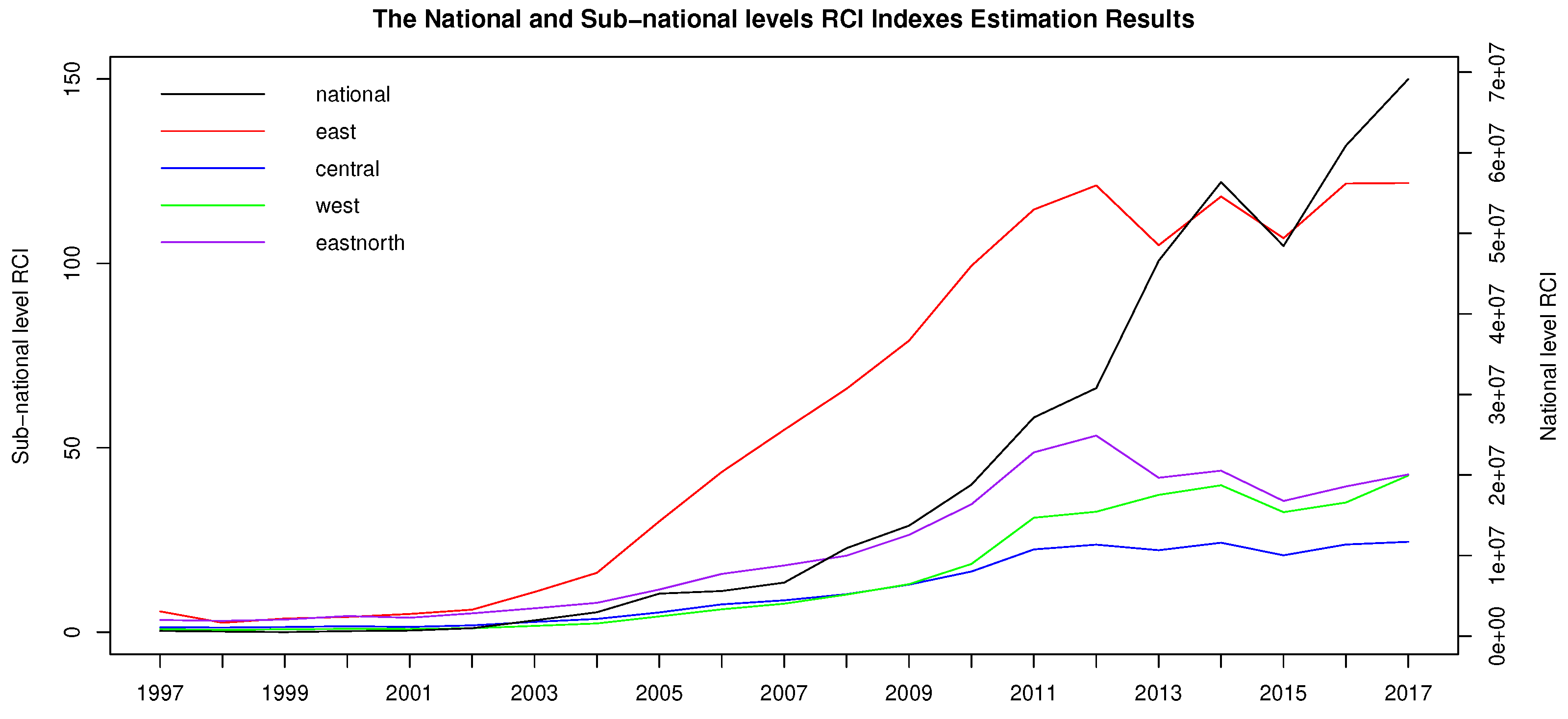
5.1.2. The National and Sub-National Levels RCI Estimation Results

In this section, we try to answer two research questions. First, from the national-level perspective, what are the characteristics of carbon inequality among provinces? Second, from the sub-national-level perspective, what are the characteristics of carbon inequality among counties? (At the sub-national level, there are four “great sub-national-regions” (east, central, west, and northwest) in China. The division of four sub-national-level regions in this paper is according to regional classification criteria of the National Bureau of Statistics of China (NBSC, see details in http://www.stats.gov.cn/tjfw/tjzx/tjzxbd/201811/t20181110_1632622.html, accessed on 10 November 2018)). The first question is the inter-provincial RCI evaluation, while the second one is the intra-sub-national-regions RCI evaluation. To explore the first question, we need the provincial emission panel data which is offered by Shan et al. (2016) [50], Shan et al. (2018) [51], Shan et al. (2020) [52], and Guan et al. (2021) [53], and is introduced in Section 3. To investigate the second question, we need to classify all county-level administrative units based on the sub-national-regions according to the classification standard of NBSC, and then all counties in the same sub-national-region are formed into a new sub-sample for further study. Both of the observations are fitted with the EGB2 distribution and the corresponding RCI indexes are computed.

The national-level carbon inequality results are shown in the second column of

Table 7. The inter-provincial carbon inequality estimation results of original carbon emission data for the nation and the east, central, west and northeast four regions in China from 1997 to 2017. For the division criteria of China’s four regions, please refer to NBSC, see details in http://www.stats.gov.cn/tjfw/tjzx/tjzxbd/201811/t20181110_1632622.html, accessed on 10 November 2018).

Year	National	East	Central	West	Northeast
1997	647,982.509	5.626	1.316	0.800	3.293
1998	568747.568	2.546	1.228	0.593	3.057
1999	498,678.736	3.688	1.377	0.757	3.408
2000	621,820.460	4.117	1.594	0.876	4.371
2001	690,551.642	4.926	1.413	0.848	3.898
2002	983,689.255	6.093	1.829	1.051	5.097
2003	1957210.067	10.890	2.776	1.685	6.465
2004	296,8701.161	16.084	3.581	2.350	7.944
2005	527,8385.658	30.060	5.348	4.264	11.562
2006	5601725.844	43.438	7.529	6.187	15.791
2007	664,6945.263	54.866	8.624	7.706	18.084
2008	1092,2095.713	66.015	10.286	10.181	20.732
2009	13712173.278	79.048	12.893	13.005	26.387
2010	18802871.775	99.347	16.435	18.487	34.666
2011	27144148.391	114.616	22.426	31.024	48.752
2012	3078,8302.103	121.153	23.723	32.655	53.300
2013	4659,6107.642	104.930	22.211	37.224	41.868
2014	5636,2173.278	118.145	24.248	39.820	43.792
2015	4843,4659.060	106.846	20.834	32.534	35.569
2016	6088,3347.545	121.666	23.764	35.146	39.508
2017	6914,8049.601	121.807	24.500	42.477	42.758

. The national RCI value decreased slightly from 1997 to 1999, but was relatively stable during this period. From 1999 to 2017, except for a slight decrease in 2015, it maintained an upward trend and peaked in 2017. It is worth noting that compared with the intra-provincial RCI values reported in Section 5.1.1, the magnitude of the national RCI index is extremely large (the order of magnitude reached ${10}^7$). This means that, nationally, the inter-provincial carbon emission inequality is much greater than that at intra-provincial level.

The sub-national-level RCI results are listed in columns 3 to 6 of Table 7. From the perspective of time, the trends of RCI indexes in the four sub-national regions are consistent. The RCI indexes decreased from 1997 to 1998, and maintained an upward trend from 1998 to 2012. From 2012 to 2017, the RCI indexes kept stable or fluctuated slightly. From the perspective of region, during the sample period 1997–2017, the RCI index of the east region remained the highest among the four sub-national regions, followed by the northeast, then the west, and the central region. The RCI index of the east region was relatively stable from 1997 to 2002, continuously rising from 2002 to 2012, and slightly fluctuating after 2012. The RCI index of the northeast region kept increasing in 1997–2012, and declined slightly in 2012–2017. The RCI index of the central and west regions were always lower than that of the east and northeast regions from 1997 to 2017. Before 2008, the RCI index of the central region was slightly higher than that of the west region; after 2008, the RCI index of the central region was relatively flat, while that of the west is always higher than the center and kept rising to the same level as the northeast region in 2017.

The resulting RCI indexes from both national and sub-national levels are plotted in Figure 1 with line curves. As can be seen from the figure, in general, the east region has the largest regional carbon inequality, while the central region is the most spatially carbon-equal region. The trend of the national RCI index is relatively similar to that of the eastern region. All RCI indexes are relatively stable from 1997 to 2002, and then kept rising from 2002 to 2012. After that, despite a slight drop in 2015, the national RCI index kept rising until 2017. The RCI index of the east region exceeded 100 and was much higher than the other three sub-national regions. The RCI index of the northeast and west were close, both around 40, with a slightly decreasing trend in the northeast and a slightly increasing trend in the west. The RCI index in the central was the lowest, at around 20, and the change was relatively flat.

5.2. Ungrouped Dependence Estimation Results

In this section, we present the ungrouped dependence estimation results for: (1) the overall dependence using copula functions and Kendall’s $\tau$; and (2) the tail dependence using TQCC.

5.2.1. Overall Dependence Estimation Results: Copula Functions

To detect whether or not there exists nonlinear dependence between the regional carbon inequality and the corresponding carbon efficiency, we utilize Kendall’s $\tau$ which is a copula-based correlation coefficient to measure the overall dependence. In this subsection, the resulting RCI indexes results in Section 5.1.1 are used as the measure of regional carbon inequality, and the regional carbon efficiency data generated by Ning et al. (2021) [54] is used as the measure of carbon efficiency. Both of the data are panel data for 30 provinces in China over the time span of 2007–2016.

In this paper, we obtain the selected copula by calling the BiCopSelect function and compute the corresponding value of Kendall’s $\tau$ of the selected copula by calling the BiCopPar2Tau function. These two functions are both available in the R package VineCopula.

Table 8. The selected optimal copula estimation between RCI and carbon efficiency for each year from 2007 to 2016.

	Original	3-Year	4-Year	5-Year
2007	Survival BB7	Survival BB7	Survival BB7	Survival BB7
2008	Survival BB7	Survival BB7	Survival BB7	Survival BB7
2009	Survival BB7	Survival BB7	Survival BB7	Survival BB7
2010	Survival BB7	Survival BB7	Survival BB7	Survival Clayton
2011	Survival Clayton	Survival Clayton	Survival BB7	Joe
2012	Joe	Joe	Joe	Joe
2013	Survival Clayton	Survival Clayton	Survival BB7	Survival Clayton
2014	Survival Clayton	Survival Clayton	Survival Clayton	Survival Clayton
2015	Joe	Joe	Joe	Joe
2016	Joe	Joe	Joe	Joe

lists the selected optimal copula estimation between carbon inequality and carbon efficiency for each year from 2007 to 2016. The corresponding Kendall’s $\tau$ estimation results and the p-values between carbon inequality and carbon efficiency for each year from 2007 to 2016 are reported in

Table 9. The Kendall’s $\tau$ estimation between RCI and carbon efficiency for each year from 2007 to 2016.

		2007	2008	2009	2010	2011	2012	2013	2014	2015	2016
original	$\tau$	0.437	0.444	0.437	0.431	0.327	0.339	0.317	0.320	0.333	0.276
	p-value	0.014	0.014	0.012	0.009	0.054	0.044	0.033	0.037	0.019	0.090
3-year	$\tau$	0.436	0.470	0.447	0.441	0.363	0.368	0.346	0.333	0.333	0.279
	p-value	0.014	0.008	0.009	0.006	0.029	0.031	0.021	0.028	0.023	0.084
4-year	$\tau$	0.446	0.455	0.444	0.441	0.375	0.368	0.360	0.338	0.347	0.277
	p-value	0.011	0.010	0.009	0.006	0.035	0.031	0.017	0.028	0.019	0.104
5-year	$\tau$	0.422	0.443	0.446	0.389	0.360	0.378	0.364	0.346	0.353	0.293
	p-value	0.010	0.010	0.009	0.009	0.020	0.021	0.019	0.023	0.017	0.090

. We also plot the Kendall’s $\tau$ estimation results in Figure 2.

As can be seen from Table 9 and Figure 2, the overall dependence (Kendall’s $\tau$) structures share a lot in common and have similar patterns under the 3-, 4-, 5-year rolling windows and the non-rolling case, which demonstrates the robustness of our results. The main findings of the overall dependence estimations are summarized as follows. On the ond hand, according to Table 9, all Kendall’s $\tau$ are significantly positive, which means that as the carbon efficiency goes up, the carbon emission tends to be more unequal within a given area. From the economic perspective, this result is particularly worthy of our attention, because it evidences that there is a very strong (statistically significant) “trade-off” between carbon efficiency and carbon inequality. Nevertheless, to achieve the economic sustainability and contribute to carbon neutrality, we must deal with this “trade-off”, and try to maintain carbon efficiency and regional carbon equality at the same time. Ideally, in terms of carbon neutral aim, it is supposed that an increase in carbon efficiency comes with less regional carbon inequality, that is, a negative value in Kendall’s $\tau$. In this sense, regional “grouping” and regional coordination might need to be discussed (see Section 5.3.2), based on which possible policy implications can be offered (see Section 6). On the other hand, however, as can be seen from Figure 2, almost all of Kendall’s $\tau$ values are decreasing over time, suggesting that the positive correlation between the RCI values and regional carbon efficiency generally weakens over time. This evidence may indicate that the above “trade-off” between carbon efficiency and carbon equality, though does exist, is becoming less “obtrusive” over time. In this regard, possible reasons are the utilization of clean energy, the development of green innovations, and their implementation in both green and non-green industries (Calza et al., 2017; Yuan et al., 2020; Lin et al., 2022) [69,70,71].

5.2.2. Tail Dependence Estimation: The TQCC Results

Based on the resulting RCI indexes and the carbon efficiency data, we compute the TQCC of each pair by Equation (7) for further studying tail dependence relationships between two variables. Theoretically, the larger the TQCC, the more severe the tail dependence (Zhang et al., 2017) [64]. In this study, the random threshold is taken as the larger one of each sequence’s upper 10%, 20%, and 30% quantiles.

Table 10. The TQCC estimation between RCI (non-rolling window) and regional carbon efficiency from 2007 to 2016 with $uq$ = 0.9, 0.8 and 0.7.

		2007	2008	2009	2010	2011	2012	2013	2014	2015	2016
0.9	$q_{u_n}$	0.334	0.365	0.346	0.328	0.251	0.276	0.283	0.239	0.304	0.315
	p-value	0.000	0.000	0.000	0.001	0.005	0.002	0.002	0.006	0.001	0.001
0.8	$q_{u_n}$	0.328	0.347	0.328	0.290	0.238	0.257	0.256	0.211	0.278	0.288
	p-value	0.001	0.000	0.001	0.002	0.006	0.004	0.004	0.013	0.002	0.002
0.7	$q_{u_n}$	0.328	0.344	0.328	0.289	0.238	0.257	0.256	0.211	0.276	0.265
	p-value	0.001	0.000	0.001	0.002	0.006	0.004	0.004	0.013	0.002	0.003

presents the TQCC estimation between regional carbon inequality and carbon efficiency and the corresponding p-values when $uq$ is equal to $0.9$, $0.8$, and $0.7$, respectively.

Table 11. The TQCC estimation between RCI (based on a 3-year rolling window) and regional carbon efficiency from 2007 to 2016 with $uq$ = 0.9, 0.8 and 0.7.

		2007	2008	2009	2010	2011	2012	2013	2014	2015	2016
0.9	$q_{u_n}$	0.338	0.363	0.367	0.341	0.323	0.306	0.308	0.271	0.277	0.311
	p-value	0.000	0.000	0.000	0.000	0.001	0.001	0.001	0.003	0.002	0.001
0.8	$q_{u_n}$	0.337	0.356	0.352	0.314	0.279	0.269	0.300	0.263	0.252	0.279
	p-value	0.000	0.000	0.000	0.001	0.002	0.003	0.001	0.003	0.004	0.002
0.7	$q_{u_n}$	0.337	0.355	0.352	0.313	0.279	0.269	0.300	0.263	0.252	0.257
	p-value	0.000	0.000	0.000	0.001	0.002	0.003	0.001	0.003	0.004	0.004

,

Table 12. The TQCC estimation between carbon inequality (based on a 4-year rolling window) and regional carbon efficiency from 2007 to 2016 with $uq$ = 0.9, 0.8 and 0.7.

		2007	2008	2009	2010	2011	2012	2013	2014	2015	2016
0.9	$q_{u_n}$	0.350	0.370	0.369	0.360	0.322	0.315	0.345	0.276	0.265	0.294
	p-value	0.000	0.000	0.000	0.000	0.001	0.001	0.000	0.002	0.003	0.001
0.8	$q_{u_n}$	0.350	0.366	0.358	0.338	0.276	0.274	0.327	0.274	0.253	0.259
	p-value	0.000	0.000	0.000	0.000	0.002	0.002	0.001	0.002	0.004	0.004
0.7	$q_{u_n}$	0.350	0.365	0.358	0.338	0.276	0.274	0.327	0.274	0.253	0.239
	p-value	0.000	0.000	0.000	0.000	0.002	0.002	0.001	0.002	0.004	0.006

and

Table 13. The TQCC estimation between RCI (based on a 5-year rolling window) and carbon efficiency from 2007 to 2016 with $uq$ = 0.9, 0.8 and 0.7.

		2007	2008	2009	2010	2011	2012	2013	2014	2015	2016
0.9	$q_{u_n}$	0.341	0.363	0.357	0.354	0.315	0.334	0.340	0.310	0.294	0.312
	p-value	0.000	0.000	0.000	0.000	0.001	0.000	0.000	0.001	0.001	0.001
0.8	$q_{u_n}$	0.341	0.357	0.348	0.336	0.277	0.291	0.312	0.300	0.288	0.293
	p-value	0.000	0.000	0.000	0.000	0.002	0.002	0.001	0.001	0.002	0.001
0.7	$q_{u_n}$	0.341	0.357	0.348	0.336	0.277	0.291	0.312	0.300	0.288	0.262
	p-value	0.000	0.000	0.000	0.000	0.002	0.002	0.001	0.001	0.002	0.003

report the TQCC results based on the rolling window period of 3, 4 and 5 years, respectively.

Using 0.334 (the TQCC value for original data in 2007 at 0.9 quantile) as an example, it means there is a 33.4% chance that given the carbon efficiency reaches an extremely high level, the RCI index reaches its extremely high level at the same time. Other TQCC values are interpreted similarly.

As can be seen from Table 10, Table 11, Table 12 and Table 13, all the p-values of TQCC results are far less than 0.05, which suggests all the TQCC results are highly significant. It illustrates that extremely spatially unequal carbon emissions also typically occur in areas with extremely high carbon efficiency.

We also plot the TQCC measures in Figure 3, which provides evidence of the dynamic tail dependence patterns between the RCI index and carbon efficiency. As can be seen from panel (a) of Figure 3, the TQCC was relatively stable from 2007 to 2009. From 2009 to 2015, except for a slight increase in 2013, TQCC decreased as a whole. From 2015 to 2016, the TQCC increased slightly again. It indicates that the change of the tail dependence probably reached empirical lower bounds which are approximately 0.28 ($uq=0.9$) and 0.25 ($uq=0.8$ and $0.7$) in 2015.

The robustness of the dynamic tail dependence results can be demonstrated by the following two empirical facts: (1) the dynamic TQCCs have similar patterns under the original data and 3-, 4-, and 5-year rolling windows; and (2) all TQCCs series have consistent trends under various values of the threshold.

The TQCC results provide empirical evidence for the existence of tail dependence between carbon efficiency and regional carbon inequality. The significant positive TQCC means that extremely higher efficiency for carbon emissions in a region is likely to come with a higher variation of carbon emissions within that area. This result shows consistency with the overall dependence results in Section 5.2.1. This provides further evidence for the carbon efficiency and carbon equality “trade-off” in tail regions, which may not be an “optimistic” situation. However, as the TQCCs in Figure 3 generally decrease in time, the “pessimistic trade-off” is becoming less urgent, probably due to the same reasons as the decreasing of the Kendall’s $\tau$ (see Section 5.2.1). The resulting fact, together with the overall dependence results, inspire us to do further discussion and grouping study, which may provide additional information for dealing with the efficiency-equality (E-E) “trade-off” (see Section 5.3).

5.3. Grouped Dependence Estimations

The ungrouped dependence estimation results in Section 5.2 evidence of an efficiency-equality (E-E) trade-off phenomenon, which means higher regional carbon efficiency tends to come with larger carbon inequality. Motivated by these empirical facts, this section aims to further investigate how we can alleviate the “E-E” conflict by grouping provincial administrations based on some variables and/or benchmarks.

Regarding the “E-E” trade-off, a natural and beautiful vision is that we can have an increase in carbon efficiency and a decrease in carbon inequality at the same time. In this regard, measuring and calculating “the carbon inequality cost for carbon efficiency” is crucial. In Section 5.3.1, we define a novel economic variable, which is termed “the carbon inequality cost for carbon efficiency,” so as to evaluate the “economic impact” of the “E-E trade-off” over regions, thereby making the economic grouping feasible and possible.

Meanwhile, in the literature, one of the major processes for carbon neutrality is industrial upgrading (Sun et al., 2022) [72]. In this process, the ratio of the added value of the tertiary industry to GDP is an important indicator of transformation (Xu et al., 2022; Zhang et al., 2022) [73,74]. Motivated by these studies, we use industrial structure (the proportion of the tertiary industry) as our second grouping variable (see Section 5.3.2).

In each subsection of this section, we group the 30 provincial administrative units into 5 groups. The grouping process is based on the idea which is to make the combination of “strongest + weakest”, that is, the regions with the lowest values in a grouping variable (the “E-E” cost, or the industrial structure) and the regions with the highest values are grouped in a pair. This grouping strategy is in line with the “the strong lead the weak” idea. Detailed rankings for the “E-E cost” and “industrial structure” are listed in

Table A13. The “E-E cost” rank of 30 provinces in China.

Province	The E-E Cost	Rank
Yunnan	−0.355	1
Sichuan	−0.326	2
Xinjiang	0.350	3
Zhejiang	0.497	4
Jiangxi	0.594	5
Hunan	0.694	6
Guangxi	0.790	7
Guizhou	0.850	8
Anhui	0.954	9
Shaanxi	0.978	10
Jilin	0.978	11
Inner Mongolia	1.011	12
Liaoning	1.062	13
Gansu	1.147	14
Guangdong	1.216	15
Shanghai	1.258	16
Ningxia	1.330	17
Shanxi	1.334	18
Shandong	1.354	19
Hebei	1.544	20
Jiangsu	1.548	21
Henan	1.562	22
Hainan	1.594	23
Heilongjiang	1.672	24
Qinghai	1.724	25
Fujian	1.754	26
Tianjin	1.932	27
Chongqing	2.229	28
Beijing	2.289	29
Hubei	4.169	30

and

Table A14. The industrial structure (the proportion of the tertiary industry) rank of 30 provinces in China.

Province	The Proportion of the Tertiary Industry	Rank
Henan	0.539	1
Qinghai	0.538	2
Shaanxi	0.530	3
Inner Mongolia	0.522	4
Shanxi	0.522	5
Jiangxi	0.520	6
Shandong	0.519	7
Hebei	0.517	8
Anhui	0.508	9
Tianjin	0.508	10
Jilin	0.505	11
Jiangsu	0.505	12
Fujian	0.504	13
Liaoning	0.502	14
Chongqing	0.500	15
Zhejiang	0.499	16
Ningxia	0.490	17
Guangdong	0.479	18
Sichuan	0.477	19
Hubei	0.470	20
Guangxi	0.456	21
Hunan	0.450	22
Xinjiang	0.446	23
Gansu	0.438	24
Heilongjiang	0.429	25
Yunnan	0.419	26
Guizhou	0.393	27
Shanghai	0.383	28
Hainan	0.264	29
Beijing	0.224	30

, respectively. Overall dependence is re-investigated by using the copula method for each grouping case. (Since TQCC can only generate non-negative values which measure the upper tail dependence, but in this section, we hope to explore the correlation from the lower tail direction, the TQCC estimation is omitted for grouped cases).

5.3.1. Grouped Dependence by “E-E Cost”

Motivated by the empirical findings in Section 5.2 which evidence an efficiency-equality (E-E) trade-off in the sample period, this section proposes a novel economic concept (variable) as the grouping criterion in this subsection for re-investigating the dependence. The variable is called “the carbon inequality cost for carbon efficiency” (or for short, the E-E cost), (“The carbon inequality cost for carbon efficiency” is the cost due to the existence of E-E trade-off, therefore we term it as “E-E cost”). and it is defined as follows:

$${E-E~Cost}_i=ln\left(\frac{{Inequality}_{i,2016}}{{Inequality}_{i,2007}}\right)-ln\left(\frac{{Efficiency}_{i,2016}}{{Efficiency}_{i,2007}}\right),$$

(8)

where ${Inequality}_{i,2016}$ and ${Inequality}_{i,2007}$ represent the carbon inequality index of province i in 2016 and 2007, respectively; and ${Efficiency}_{i,2016}$ and ${Efficiency}_{i,2007}$ represent the carbon efficiency of province i in 2016 and 2007, respectively. This construction is inspired by the connotation “log-return” in empirical finance, which is commonly used in financial literature as a measure of the change of a time series value from an initial time point to an end time point. In this paper, the initial and the end time points are 2007 and 2016, respectively. Consequently, the economic meaning of Equation (8) is essentially the gap between the change of carbon inequality index and the change of carbon efficiency in the region i over the whole sample period. Theoretically, the larger value in Equation (8), the greater the “carbon inequality cost for carbon efficiency”. It is worth noting that a negative value in E-E cost of the region i means an increase in carbon emission efficiency and an increase in carbon equality can be achieved in the region i simultaneously. The E-E cost results of 30 provincial administrative units in China are shown in Table A13.

Based on the “strongest + weakest” grouping strategy, we select 3 units from the highest and another 3 units from the lowest according to the E-E cost values in turn to form groups and eventually divide 30 provincial administrative units into 5 groups. Group numbers 1–5 represent intra-group differences from the largest to the smallest. Consequently, We re-investigate the overall dependence for each group using copula functions and calculate the corresponding Kendall’s $\tau$. The grouping results and grouped Kendall’s $\tau$ are shown in

Table 14. The grouping results according to the E-E cost, and Kendall’s $\tau$ estimation between RCI and regional carbon efficiency for the six provinces in each group. Group numbers 1–5 represent intra-group differences from the largest to the smallest. ${}^{***}$ stands for statistical significance at 1% level.

	Group 1	Group2	Group 3	Group 4	Group 5
Provinces	Yunnan	Xinjiang	Guangxi	Shaanxi	Liaoning
	Sichuan	Zhejiang	Guizhou	Jilin	Gansu
	Xinjiang	Jiangxi	Anhui	InnerMongolia	Guangdong
	Chongqing	Qinghai	Henan	Shandong	Shanghai
	Beijing	Fujian	Hainan	Hebei	Ningxia
	Hubei	Tianjin	Heilongjiang	Jiangsu	Shanxi
Rank	1, 2, 3,	4, 5, 6,	7, 8, 9,	10, 11, 12,	13, 14, 15,
	28, 29, 30	25, 26, 27	22, 23, 24	19, 20, 21	16, 17, 18
Kendall’s $\tau$	$0.444{}^{***}$	$0.670{}^{***}$	$-0.578{}^{***}$	−0.117	$0.506{}^{***}$
p-value	$1.366\times {10}^{-5}$	$1.255\times {10}^{-13}$	$1.548\times {10}^{-10}$	0.677	$2.147\times {10}^{-8}$

.

According to Table 14, we may dig out the evidence for coordinating the “E-E” trade-off and offering implications for carbon neutrality. We find that the Kendall’s $\tau$ estimation of the third and fourth groups are negative, indicating that the higher carbon efficiency comes with more balanced regional carbon emission in these groups. Even though the dependence in Group 4 is insignificant, we should note that this at least indicates that the “E-E” trade-off can be eliminated in areas of Group 4 by grouping via E-E cost. This result means that by re-formulating the regional coordinating strategy according to certain benchmarks (by the order of the proposed E-E cost in this case), both carbon equality and carbon efficiency can be achieved in some regions simultaneously.

Based on the previous research, the above empirical result can be interpreted from the following two aspects. First, regional economic cooperation and integration can decrease carbon dioxide marginal abatement costs by providing the facility for the movement of labor and capital (Xu and Voon, 2003; Daniel and DeJong, 2003; Kumar et al., 2014) [75,76,77], thereby improving the efficiency of energy utilization and energy management at the economic level (even if their technical efficiency remains the same). Second, by “grouping” and integrating areas, there would be positive network externalities on local production and carbon emission technology (Wang and He, 2017; He et al., 2018) [78,79], both of which are conducive to the improvement of carbon emission efficiency (positive effect on carbon efficiency) and factor equalization (positive effect on carbon equality).

This empirical evidence provides us with at least three inspirations: (1) the regional economic restructuring planning according to some variables with important economic connotations is an important idea to reconcile the “efficiency–equality” trade-off and achieve green development; (2) the E-E cost proposed in this paper and its economic connotation can be used as a reference in the process of broader emission reduction and carbon neutrality policies; (3) more reference variables (such as industrial structure which would be discussed in Section 5.3.2) that may be used as the regional economic planning can be proposed and related empirical research can be conducted.

5.3.2. Grouped Dependence by Industrial Structure

The empirical evidence in Section 5.3.1 implies the significance of the regional planning and re-grouping strategy, which inspires us to look for more possibilities for solving the E-E trade-off. According to recent studies, the increase of the tertiary industry’s proportion in economy is an important feature of cleaner production, green economy development, and carbon emission efficiency improvement (Sun et al., 2022; Xu et al., 2022; Zhang et al., 2022) [72,73,74]. In this subsection, we use industrial structure as a grouping variable to re-investigate the dependence of regional carbon efficiency and regional carbon inequality within each grouped region.

The grouping variable industrial structure is an indicator of the proportion of the tertiary industry in the regional economy, which is defined as:

$${Industrial\; structure}_i=\frac{{The\; added\; value\; of\; the\; tertiary\; industry}_i}{{GDP}_i}$$

(9)

where i represents the ith province. The original data for computing industrial structure is downloaded from the National Bureau of Statistics of China’s website (https://data.stats.gov.cn/easyquery.htm?cn=E0103, (accessed on 1 January 2018)). The computed industrial structure values for the 30 provincial administrative units are listed in Table A14.

The grouping method for industrial structure is analog to that in Section 5.3.1, that is, the combination of the “strongest + weakest” pairs. By doing so, we divide 30 provincial administrative units into 5 groups according to the rank of industrial structure values. The grouping results according to the industrial structure and the overall dependence Kendall’s $\tau$ for each group are shown in

Table 15. The grouping results according to the industrial structure, and Kendall’s $\tau$ estimation between carbon inequality and carbon efficiency for the six provinces in each group. Group numbers 1–5 represent intra-group differences from the largest to the smallest. *** stands for statistical significance at 1% level. ** stands for statistical significance at 5% level.

	Group 1	Group 2	Group 3	Group 4	Group 5
Provinces	Henan	InnerMongolia	Shandong	Tianjin	Fujian
	Qinghai	Shanxi	Hebei	Jilin	Liaoning
	Shaanxi	Jiangxi	Anhui	Jiangsu	Chongqing
	Shanghai	Heilongjiang	Hunan	Sichuan	Zhejiang
	Hainan	Yunnan	Xinjiang	Hubei	Ningxia
	Beijing	Guizhou	Gansu	Guangxi	Guangdong
Rank	1, 2, 3,	4, 5, 6,	7, 8, 9,	10, 11, 12,	13, 14, 15,
	28, 29, 30	25, 26, 27	22, 23, 24	19, 20, 21	16, 17, 18
Kendall’s $\tau$	$0.438{}^{***}$	$-0.378{}^{***}$	−0.194	$0.551{}^{***}$	$0.244{}^{**}$
p-value	$1.720\times {10}^{-6}$	$2.645\times {10}^{-4}$	0.409	$2.645\times 4.{196}^{-9}$	0.014

.

As can be seen from Table 15, the Kendall’s $\tau$ estimation of the second and third groups are negative, suggesting that both carbon equality and carbon efficiency are achieved in these grouping areas. In Group 3, the negative dependence is insignificant, which means the “win-win” result may not be that strong. However, the insignificance can still imply that the dilemma of “E-E trade-off” can be solved in the areas in Group 3. This empirical result is in line with the evidence provided by Sun et al. (2022), Xu et al. (2022), and Zhang et al. (2022) [72,73,74] who believe that the upgrading of industrial structure is an important way to improve regional carbon emission efficiency and energy efficiency, and has very little spatial and/or industrial negative externalities. In the context of this subsection, the specific embodiment of negative spatial externality is that the improvement of carbon emission efficiency may lead to an increase in carbon emission inequality. Obviously, after using industrial structure variables for regional grouping, the negative externalities in some regions (Groups 2 and 3) disappeared, and even some regions (Group 2) saw evidence of positive environmental externalities.

The empirical results in this subsection once again confirm the necessity of the regional economic planning in alleviating the contradiction between the E-E trade-off of carbon emissions and its important role in achieving carbon neutrality. It is worth mentioning that in both grouping studies using industrial structure in this subsection and using E-E cost in Section 5.3.1, the regions that show the “good result”, that is, the positive dependence between the RCI and carbon efficiency disappears, only exists in the “middle” of the grouping list (i.e., Group 2, 3, and/or 4). Does this mean that the ability or the “power” of solving “E-E trade-off” by using regional economic regrouping strategies is only applicable to the situations where the differences within the group are not particularly small or large? The authors believe that, however, based on the evidence in this article and the existing literature, we cannot yet draw this conclusion. This is because we currently have insufficient grouping variables for computing copula-based grouping dependence. There are possibilities that the above results are just special cases of the grouping variables E-E cost and industrial structure using the sample data in this paper. In the future, it would be interesting and of both academic and practical significance to investigate if the “middle is good” phenomenon still exists in cases using other grouping variables or/and other datasets.

6. Conclusions, Implications, and Future Research Directions

6.1. Main Findings

This paper proposes a novel regional carbon emission inequality (RCI) index based on the EGB2 distribution. Using the proposed RCI index and based on China’s county-level panel data, the carbon emission inequality of China is measured at three levels: intra-provincial, sub-national, and national. Based on the resulting RCI indexes, the dependence between regional carbon efficiency and carbon inequality is investigated by using copula functions and TQCC. The major findings of our study are as follows. First, the proposed regional carbon inequality index suggests that Shanghai, Tianjin, and Inner Mongolia have the worst carbon inequalities (i.e., the highest values in RCI indexes); while Hainan, Qinghai, and Jiangxi are the three most carbon-equal provinces (i.e., with the lowest RCI values). The rank of the regional distribution of carbon emission inequality has no obvious relationship with the geographical distribution of each province. Second, an interesting divergence phenomenon in RCI values can be found in municipalities over the past decade. Third, from a national-level perspective, the inter-provincial carbon emission inequality is much greater than that at the intra-provincial level. From the sub-national-level perspective, the east region has the highest degree of carbon emission inequality among the four sub-national-level regions, and is much higher than the other three sub-national-level regions, followed by the northeast region; and the central region is relatively the most balanced one. Fourth, both the overall and tail dependence between the regional carbon efficiency and carbon inequality are significantly negative for all ungrouped cases, suggesting that there is a so-called “efficiency-equality (E-E) trade-off” in each provincial administrative unit, which means the higher carbon efficiency generally come with higher carbon inequality within a province. Finally, regarding the so-called “E-E trade-off”, this paper also proposes a novel concept, the efficiency–equality (E-E) cost, which can be used as a grouping variable for regional economic planning and coordination. The grouped results show that by re-grouping provincial units via the proposed variable E-E cost and industrial structure, some of the “middle groups” (Group 2, 3, and 4) display negative Kendall’s $\tau$ values, which means that both carbon equality and carbon efficiency can be achieved in some of the areas simultaneously, thereby solving the “E-E trade-off” problem. This result also implies the necessity of the regional coordinating strategy and thus may offer some important implications for policy-makers.

6.2. Policy Implications

Regarding the above empirical findings, especially the notable difference between the grouped and ungrouped results, the following policy implications can be offered.

First, the regional economic planning and coordination are important policy tools for solving dilemmas regarding the welfare issues of the environmental problems. In this paper, the grouping strategy is used to solve the “efficiency-equality” trade-off. Essentially, this is one of the concrete manifestations of the economic topic of the relationship between efficiency and fairness in the environmental field. Regarding this topic, the authors believe that the ideas of “grouping” and “the strong lead the weak” can be applied in various dimensions (not just dealing with environmental efficiency and equality). For example, establishing a cross-regional carbon emission indicator trading market to optimize the allocation of carbon emission rights. Meanwhile, the government can lead “cleaner-production-tech” leasing projects between the “strongest” and “weakest” regions, and provide the enterprises in the “strongest” regions with economic support such as tax reduction.

Second, the E-E cost proposed in this paper and its economic connotation can be generalized as references for regional coordination in wider realms, such as the policy-making process regarding cleaner production, emission reduction, and carbon neutrality. In fact, using the “difference of logarithmic rate of return” construction, the police-makers can generalize many carbon emission economic evaluation indicators (variables). As long as the proposed indicator can be computed by “changes in environmental cost” mines “changes in environmental benefit”, it can be used in the evaluation of environmental policy implementation.

Last but not least, more reference variables can be investigated and used as a reference for regional economic coordination. In Section 5.3, we use E-E cost, and industrial structure as grouping variables. Admittedly, however, we cannot be sure that these two grouping variables are the “optimal” grouping variables - in fact, due to the fact that environmental and economic variable distributions change over time and vary by region (i.e., the spatial fixed effect, see Lin et al. (2022) [71]), there may not be an “optimal” grouping variable for all regions at any time. In practice, in order to reduce the cost of implementation, the central government can coordinate with local governments, and take the “greatest common divisor” of the resources urgently needed by each region in demand for cleaner production for cross-regional coordination, so as to propose a “second-best” but feasible grouping variable.

6.3. Limitations and Future Research

Regarding the empirical findings, there might be some interesting stuff left for future research.

First, the RCI index proposed in this paper is an “absolute” measure of carbon inequality at the spatial level. Nevertheless, the possible causes of inequality have not been studied. In the future, further studies can utilize the proposed RCI index as a dependent variable, and its driven factors can be further investigated. In this regard, spatial econometrics is a suitable methodology.

Second, in Section 5.1.1, we find an interesting divergence of RCI indexes in municipalities. Regarding this result, one might be curious about whether this phenomenon could be explained by the industrial structural changes and the differences in the functional positioning of municipalities over the past few years. This can be left as an interesting topic for urban economic study.

Third, the grouping dependence results in Section 5.3 exhibit a “middle is good” (the “E-E trade-off” is only solved in groups with moderate within group variation, that is, Group 2, 3, or/and 4) phenomenon in each case. It would be interesting to figure out if this phenomenon still exists by using other grouping variables and/or other datasets.

Fourth, whereas our empirical findings provide evidence for the existence of “E-E trade-off”, its economic mechanism is not mentioned. Actually, there can be multi-factors driving this phenomenon, and thus the in-depth economic causality is supposed to be further discussed both theoretically and empirically.

Fifth, considering the panel data structure of the carbon emission data, we use the static EGB2 distribution for the fitting. That is, each region (no matter for provincial, sub-national, or national) is fitted year by year. However, this is just the first step for a related study. Recently, the dynamic EGB2 model (Caivano and Harvey, 2014) [80] and the dynamic time series model of other asymmetric distributions such as dynamic Weibull (Deng et al., 2020) [48] have been proposed by econometric scholars. These novel methodologies may be conducive to further study of related topics based on the proposed RCI index and the research framework of this paper.

Sixth, due to the lack of enough (more than 5 years) most recent county-level panel data, in this paper, we are not able to conduct the research based on the latest carbon emission information. There are possibilities that the recent carbon emissions in China might be slightly different from that before the year 2020. (In the year 2020, China pledged to be carbon neutral by 2060, thereby leading to the introduction of many policies for supporting Chinese green industries and green innovations). However, based on existing theories, we cannot yet conclusively say whether the dependence results today are higher or lower than the dependence estimates in the sample period of this paper. There is even a possibility that the dependencies before and after 2020 are not significantly different, even if green innovations and green industries are indeed supported. Thus, this comparable study can be left for future study when enough data (at least 5 years) is released. Regarding this issue, many contemporary econometric methods such as segmented multivariate regression (Liu et al., 1997) [81], max-linear regression (Cui et al., 2021) [82], and multiple time periods Difference-in-Differences (DID) approach (Callaway and Sant’anna, 2021) [83] can be used.

Finally, it would be of both academic and practical significance to investigate what other possible grouping variables can be used for regional coordination. As discussed above, there may not be an “optimal” grouping variable for all regions. Therefore, it is of great significance to find grouping variables that are applicable to different economies in practice. Specifically, possible attention can be paid on green innovation and its regional differences (Yang et al., 2020; Zhang et al., 2022; Qing et al., 2022) [84,85,86]. In this regard, the proposed RCI index and the framework used in this paper would be helpful for doing more work.

References

1. Zhao, X.; Ma, X.; Chen, B.; Shang, Y.; Song, M. Challenges toward carbon neutrality in China: Strategies and countermeasures. Resour. Conserv. Recycl. 2022, 176, 105959. [Google Scholar] [CrossRef]
2. Demirkhanyan, B. Emission Reduction Potential and Directions for Long Term Low Emission Development Framework of Armenia Transport Sector. 2020. Available online: https://eu4climate.eu/download/emission-reduction-potential-and-directions-for-long-term-low-emission-development-framework-of-armenia-transport-sector/ (accessed on 4 September 2022).
3. Dong, L.; Miao, G.; Wen, W. China’s carbon neutrality policy: Objectives, impacts and paths. East Asian Policy 2021, 13, 5–18. [Google Scholar] [CrossRef]
4. Tian, J.; Yu, L.; Xue, R.; Zhuang, S.; Shan, Y. Global low-carbon energy transition in the post-COVID-19 era. Appl. Energy 2022, 307, 118205. [Google Scholar] [CrossRef] [PubMed]
5. Vaka, M.; Walvekar, R.; Rasheed, A.K.; Khalid, M. A review on Malaysia’s solar energy pathway towards carbon-neutral Malaysia beyond COVID’19 pandemic. J. Clean. Prod. 2020, 273, 122834. [Google Scholar] [CrossRef]
6. Sadiq, M.; Nonthapot, S.; Mohamad, S.; Keong, O.C.; Ehsanullah, S.; Iqbal, N. Does green finance matter for sustainable entrepreneurship and environmental corporate social responsibility during COVID-19? China Financ. Rev. Int. 2021, 12, 317–333. [Google Scholar] [CrossRef]
7. Liu, Z.; Deng, Z.; He, G.; Wang, H.; Zhang, X.; Lin, J.; Qi, Y.; Liang, X. Challenges and opportunities for carbon neutrality in China. Nat. Rev. Earth Environ. 2022, 3, 141–155. [Google Scholar] [CrossRef]
8. Zhao, F.; Liu, X.; Zhang, H.; Liu, Z. Automobile industry under China’s Carbon peaking and carbon neutrality goals: Challenges, opportunities, and coping strategies. J. Adv. Transp. 2022, 2022, 5834707. [Google Scholar] [CrossRef]
9. Zhang, H. Technology innovation, economic growth and carbon emissions in the context of carbon neutrality: Evidence from BRICS. Sustainability 2021, 13, 11138. [Google Scholar] [CrossRef]
10. Jia, Z.; Lin, B. How to achieve the first step of the carbon-neutrality 2060 target in China: The coal substitution perspective. Energy 2021, 233, 121179. [Google Scholar] [CrossRef]
11. Zhang, P.; Hu, J.; Zhao, K.; Chen, H.; Zhao, S.; Li, W. Dynamics and decoupling analysis of carbon emissions from construction industry in China. Buildings 2022, 12, 257. [Google Scholar] [CrossRef]
12. Pan, A.; Zhang, W.; Shi, X.; Dai, L. Climate policy and low-carbon innovation: Evidence from low-carbon city pilots in China. Energy Econ. 2022, 112, 106129. [Google Scholar] [CrossRef]
13. Chi, Y.; Liu, Z.; Wang, X.; Zhang, Y.; Wei, F. Provincial CO2 emission measurement and analysis of the construction industry under china’s carbon neutrality target. Sustainability 2021, 13, 1876. [Google Scholar] [CrossRef]
14. Heil, M.T.; Wodon, Q.T. Inequality in CO2 emissions between poor and rich countries. J. Environ. Dev. 1997, 6, 426–452. [Google Scholar] [CrossRef]
15. Teixidó-Figueras, J.; Steinberger, J.K.; Krausmann, F.; Haberl, H.; Wiedmann, T.; Peters, G.P.; Duro, J.A.; Kastner, T. International inequality of environmental pressures: Decomposition and comparative analysis. Ecol. Indic. 2016, 62, 163–173. [Google Scholar] [CrossRef]
16. Padilla, E.; Duro, J.A. Explanatory factors of CO2 per capita emission inequality in the European Union. Energy Policy 2013, 62, 1320–1328. [Google Scholar] [CrossRef]
17. Hubacek, K.; Baiocchi, G.; Feng, K.; Muñoz Castillo, R.; Sun, L.; Xue, J. Global carbon inequality. Energy Ecol. Environ. 2017, 2, 361–369. [Google Scholar] [CrossRef]
18. Zhang, X.; Li, M.; Li, Q.; Wang, Y.; Chen, W. Spatial Threshold Effect of Industrial Land Use Efficiency on Industrial Carbon Emissions: A Case Study in China. Int. J. Environ. Res. Public Health 2021, 18, 9368. [Google Scholar] [CrossRef]
19. Schindler, D.; Jung, C. Copula-based estimation of directional wind energy yield: A case study from Germany. Energy Convers. Manag. 2018, 169, 359–370. [Google Scholar] [CrossRef]
20. Niemierko, R.; Töppel, J.; Tränkler, T. A D-vine copula quantile regression approach for the prediction of residential heating energy consumption based on historical data. Appl. Energy 2019, 233, 691–708. [Google Scholar] [CrossRef]
21. Gozgor, G.; Tiwari, A.K.; Khraief, N.; Shahbaz, M. Dependence structure between business cycles and CO2 emissions in the US: Evidence from the time-varying Markov-Switching Copula models. Energy 2019, 188, 115995. [Google Scholar] [CrossRef] [Green Version]
22. Fan, W.; Li, L.; Wang, F.; Li, D. Driving factors of CO2 emission inequality in China: The role of government expenditure. China Econ. Rev. 2020, 64, 101545. [Google Scholar] [CrossRef]
23. Zhong, H.; Feng, K.; Sun, L.; Cheng, L.; Hubacek, K. Household carbon and energy inequality in Latin American and Caribbean countries. J. Environ. Manag. 2020, 273, 110979. [Google Scholar] [CrossRef]
24. Cui, W.; Wan, A.; Xin, F.; Li, Q. How does carbon emission reduction efficiency affect regional income inequality? The mediator effect of interregional labor flow. Math. Probl. Eng. 2021, 2021, 5578027. [Google Scholar] [CrossRef]
25. Fang, D.; Chen, B. Inequality of air pollution and carbon emission embodied in inter-regional transport. Energy Procedia 2019, 158, 3833–3839. [Google Scholar] [CrossRef]
26. Wang, S.; Wang, J.; Fang, C.; Feng, K. Inequalities in carbon intensity in China: A multi-scalar and multi-mechanism analysis. Appl. Energy 2019, 254, 113720. [Google Scholar] [CrossRef]
27. Pan, X.; Wang, H.; Wang, Z.; Lin, L.; Zhang, Q.; Zheng, X.; Chen, W. Carbon Palma Ratio: A new indicator for measuring the distribution inequality of carbon emissions among individuals. J. Clean. Prod. 2019, 241, 118418. [Google Scholar] [CrossRef]
28. Du, Q.; Li, J.; Li, Y.; Huang, N.; Zhou, J.; Li, Z. Carbon inequality in the transportation industry: Empirical evidence from China. Environ. Sci. Pollut. Res. 2020, 27, 6300–6311. [Google Scholar] [CrossRef]
29. Mushta, A.; Chen, Z.; Ud Din, N.; Ahmad, B.; Zhang, X. Income inequality, innovation and carbon emission: Perspectives on sustainable growth. Econ. Res. Ekon. Istraživanja 2020, 33, 769–787. [Google Scholar] [CrossRef]
30. Han, M.; Lao, J.; Yao, Q.; Zhang, B.; Meng, J. Carbon inequality and economic development across the Belt and Road regions. J. Environ. Manag. 2020, 262, 110250. [Google Scholar] [CrossRef]
31. Wang, M.; Feng, C. The inequality of China’s regional residential CO2 emissions. Sustain. Prod. Consum. 2021, 27, 2047–2057. [Google Scholar] [CrossRef]
32. Zhang, S.; Wang, Y.; Hao, Y.; Liu, Z. Shooting two hawks with one arrow: Could China’s emission trading scheme promote green development efficiency and regional carbon equality? Energy Econ. 2021, 101, 105412. [Google Scholar] [CrossRef]
33. Duro, J.A. On the automatic application of inequality indexes in the analysis of the international distribution of environmental indicators. Ecol. Econ. 2012, 76, 1–7. [Google Scholar] [CrossRef]
34. Zhang, P.; You, J.; Jia, G.; Chen, J.; Yu, A. Estimation of carbon efficiency decomposition in materials and potential material savings for China’s construction industry. Resour. Policy 2018, 59, 148–159. [Google Scholar] [CrossRef]
35. Zhou, W.; Yu, W. Regional variation in the carbon dioxide emission efficiency of construction industry in China: Based on the three-stage DEA model. Discret. Dyn. Nat. Soc. 2021, 2021. [Google Scholar] [CrossRef]
36. Tan, J.; Wang, R. Research on evaluation and influencing factors of regional ecological efficiency from the perspective of carbon neutrality. J. Environ. Manag. 2021, 294, 113030. [Google Scholar] [CrossRef] [PubMed]
37. Liu, N.; Ma, Z.; Kang, J.; Su, B. A multi-region multi-sector decomposition and attribution analysis of aggregate carbon intensity in China from 2000 to 2015. Energy Policy 2019, 129, 410–421. [Google Scholar] [CrossRef]
38. Wang, B.; Yu, M.; Zhu, Y.; Bao, P. Unveiling the driving factors of carbon emissions from industrial resource allocation in China: A spatial econometric perspective. Energy Policy 2021, 158, 112557. [Google Scholar] [CrossRef]
39. Yang, B.; Wang, Z.; Zou, L.; Zou, L.; Zhang, H. Exploring the eco-efficiency of cultivated land utilization and its influencing factors in China’s Yangtze River Economic Belt, 2001–2018. J. Environ. Manag. 2021, 294, 112939. [Google Scholar] [CrossRef] [PubMed]
40. Ma, D.; Zhao, N.; Zhang, F.; Xiao, Y.; Guo, Z.; Liu, C. Green Total-factor energy efficiency of construction industry and its driving factors: Spatial-Temporal heterogeneity of Yangtze River Economic Belt in China. Int. J. Environ. Res. Public Health 2022, 19, 9972. [Google Scholar] [CrossRef] [PubMed]
41. Zhu, H.; Xia, H.; Guo, Y.; Peng, C. The heterogeneous effects of urbanization and income inequality on CO2 emissions in BRICS economies: Evidence from panel quantile regression. Environ. Sci. Pollut. Res. 2018, 25, 17176–17193. [Google Scholar] [CrossRef] [PubMed]
42. Dahal, K.; Juhola, S.; Niemelä, J. The role of renewable energy policies for carbon neutrality in Helsinki Metropolitan area. Sustain. Cities Soc. 2018, 40, 222–232. [Google Scholar] [CrossRef]
43. Liu, C.; Jiang, Y.; Xie, R. Does income inequality facilitate carbon emission reduction in the US? J. Clean. Prod. 2019, 217, 380–387. [Google Scholar] [CrossRef]
44. Mi, Z.; Zheng, J.; Meng, J.; Ou, J.; Hubacek, K.; Liu, Z.; Coffman, D.; Stern, N.; Liang, S.; Wei, Y.M. Economic development and converging household carbon footprints in China. Nat. Sustain. 2020, 3, 529–537. [Google Scholar] [CrossRef]
45. Bai, C.; Feng, C.; Yan, H.; Yi, X.; Chen, Z.; Wei, W. Will income inequality influence the abatement effect of renewable energy technological innovation on carbon dioxide emissions? J. Environ. Manag. 2020, 264, 110482. [Google Scholar] [CrossRef]
46. Tan, Y.; Uprasen, U. Carbon neutrality potential of the ASEAN-5 countries: Implications from asymmetric effects of income inequality on renewable energy consumption. J. Environ. Manag. 2021, 299, 113635. [Google Scholar] [CrossRef] [PubMed]
47. Deng, L.; Zhang, Z. Assessing the features of extreme smog in China and the differentiated treatment strategy. Proc. R. Soc. Math. Phys. Eng. Sci. 2018, 474, 20170511. [Google Scholar] [CrossRef]
48. Deng, L.; Yu, M.; Zhang, Z. Statistical learning of the worst regional smog extremes with dynamic conditional modeling. Atmosphere 2020, 11, 665. [Google Scholar] [CrossRef]
49. Chen, J.; Gao, M.; Cheng, S.; Hou, W.; Song, M.; Liu, X.; Liu, Y.; Shan, Y. County-level CO2 emissions and sequestration in China during 1997–2017. Sci. Data 2020, 7, 391. [Google Scholar] [CrossRef]
50. Shan, Y.; Liu, J.; Liu, Z.; Xu, X.; Shao, S.; Wang, P.; Guan, D. New provincial CO2 emission inventories in China based on apparent energy consumption data and updated emission factors. Appl. Energy 2016, 184, 742–750. [Google Scholar] [CrossRef]
51. Shan, Y.; Guan, D.; Zheng, H.; Ou, J.; Li, Y.; Meng, J.; Mi, Z.; Liu, Z.; Zhang, Q. China CO2 emission accounts 1997–2015. Sci. Data 2018, 5, 170201. [Google Scholar] [CrossRef] [PubMed] [Green Version]
52. Shan, Y.; Huang, Q.; Guan, D.; Hubacek, K. China CO2 emission accounts 2016–2017. Sci. Data 2020, 7, 54. [Google Scholar] [CrossRef]
53. Guan, Y.; Shan, Y.; Huang, Q.; Chen, H.; Wang, D.; Hubacek, K. Assessment to China’s recent emission pattern shifts. Earth Future 2021, 9, e2021EF002241. [Google Scholar] [CrossRef]
54. Lunchen, N.; Wen, Z.; Liang’en, Z. Research on China’s Carbon Dioxide Emissions Efficiency from 2007 to 2016: Based on Two Stage Super Efficiency SBM Model and Tobit Model. Beijing Xue Xue Bao 2021, 57, 181–188. (In Chinese) [Google Scholar]
55. Jarque, C.M.; Bera, A.K. A test for normality of observations and regression residuals. Int. Stat. Rev. Int. Stat. 1987, 55, 163–172. [Google Scholar] [CrossRef]
56. Tone, K. A slacks-based measure of efficiency in data envelopment analysis. Eur. J. Oper. Res. 2001, 130, 498–509. [Google Scholar] [CrossRef]
57. McDonald, J.B.; Xu, Y.J. A generalization of the beta distribution with applications. J. Econom. 1995, 66, 133–152. [Google Scholar] [CrossRef]
58. Kerman, S.C.; McDonald, J.B. Skewness-kurtosis bounds for EGB1, EGB2, and special cases. Commun.-Stat.-Theory Methods 2015, 44, 3857–3864. [Google Scholar] [CrossRef]
59. Coles, S.; Bawa, J.; Trenner, L.; Dorazio, P. An Introduction to Statistical Modeling of Extreme Values; Springer: Berlin/Heidelberg, Germany, 2001; Volume 208. [Google Scholar]
60. Nelsen, R.B. An Introduction to Copulas; Springer Science & Business Media: Berlin/Heidelberg, Germany, 2007. [Google Scholar]
61. Cherubini, U.; Luciano, E.; Vecchiato, W. Copula Methods in Finance; John Wiley & Sons: Hoboken, NJ, USA, 2004. [Google Scholar]
62. Sklar, M. Fonctions de repartition an dimensions et leurs marges. Publ. Inst. Statist. Univ. Paris 1959, 8, 229–231. [Google Scholar]
63. Zhang, Z. Quotient correlation: A sample based alternative to Pearson’s correlation. Ann. Stat. 2008, 36, 1007–1030. [Google Scholar] [CrossRef]
64. Zhang, Z.; Zhang, C.; Cui, Q. Random threshold driven tail dependence measures with application to precipitation data analysis. Stat. Sin. 2017, 27, 685–709. [Google Scholar]
65. Genest, C.; Rivest, L.P. Statistical inference procedures for bivariate Archimedean copulas. J. Am. Stat. Assoc. 1993, 88, 1034–1043. [Google Scholar] [CrossRef]
66. Zhang, F.; Zhang, Z. The tail dependence of the carbon markets: The implication of portfolio management. PLoS ONE 2020, 15, e0238033. [Google Scholar] [CrossRef] [PubMed]
67. Lin, H.; Zhang, Z. The impacts of digital finance development on household income, consumption, and financial asset holding: An extreme value analysis of China’s microdata. Pers. Ubiquitous Comput. 2022, 1–21. [Google Scholar] [CrossRef] [PubMed]
68. Lin, H.; Zhang, Z. Extreme co-movements between infectious disease events and crude oil futures prices: From extreme value analysis perspective. Energy Econ. 2022, 110, 106054. [Google Scholar] [CrossRef]
69. Calza, F.; Parmentola, A.; Tutore, I. Types of green innovations: Ways of implementation in a non-green industry. Sustainability 2017, 9, 1301. [Google Scholar] [CrossRef]
70. Yuan, Q.; Yang, D.; Yang, F.; Luken, R.; Saieed, A.; Wang, K. Green industry development in China: An index based assessment from perspectives of both current performance and historical effort. J. Clean. Prod. 2020, 250, 119457. [Google Scholar] [CrossRef]
71. Lin, H.; Wang, X.; Bao, G.; Xiao, H. Heterogeneous spatial effects of FDI on CO2 emissions in China. Earth Future 2022, 10, e2021EF002331. [Google Scholar] [CrossRef]
72. Sun, Y.; Liu, S.; Li, L. Grey Correlation Analysis of Transportation Carbon Emissions under the Background of Carbon Peak and Carbon Neutrality. Energies 2022, 15, 3064. [Google Scholar] [CrossRef]
73. Xu, G.; Dong, H.; Xu, Z.; Bhattarai, N. China can reach carbon neutrality before 2050 by improving economic development quality. Energy 2022, 243, 123087. [Google Scholar] [CrossRef]
74. Zhang, X.; Zheng, J.; Wang, L. Can the relationship between atmospheric environmental quality and urban industrial structure adjustment achieve green and sustainable development in China? A case of Taiyuan City. Energies 2022, 15, 3402. [Google Scholar] [CrossRef]
75. Xu, X.; Voon, J.P. Regional integration in China: A statistical model. Econ. Lett. 2003, 79, 35–42. [Google Scholar] [CrossRef]
76. Berkowitz, D.; DeJong, D.N. Regional integration: An empirical assessment of Russia. J. Urban Econ. 2003, 53, 541–559. [Google Scholar] [CrossRef]
77. Kumar, S.; Sen, R.; Srivastava, S. Does economic integration stimulate capital mobility? An analysis of four regional economic communities in Africa. J. Int. Financ. Mark. Inst. Money 2014, 29, 33–50. [Google Scholar] [CrossRef] [Green Version]
78. Wang, Z.; He, W. CO2 emissions efficiency and marginal abatement costs of the regional transportation sectors in China. Transp. Res. Part D Transp. Environ. 2017, 50, 83–97. [Google Scholar] [CrossRef]
79. He, W.; Wang, B.; Danish; Wang, Z. Will regional economic integration influence carbon dioxide marginal abatement costs? Evidence from Chinese panel data. Energy Econ. 2018, 74, 263–274. [Google Scholar] [CrossRef] [PubMed]
80. Caivano, M.; Harvey, A. Time-series models with an EGB2 conditional distribution. J. Time Ser. Anal. 2014, 35, 558–571. [Google Scholar] [CrossRef]
81. Liu, J.; Wu, S.; Zidek, J.V. On segmented multivariate regression. Stat. Sin. 1997, 7, 497–525. [Google Scholar]
82. Cui, Q.; Xu, Y.; Zhang, Z.; Chan, V. Max-linear regression models with regularization. J. Econom. 2021, 222, 579–600. [Google Scholar] [CrossRef]
83. Callaway, B.; Sant’Anna, P.H. Difference-in-differences with multiple time periods. J. Econom. 2021, 225, 200–230. [Google Scholar] [CrossRef]
84. Yang, Z.; Ali, S.T.; Ali, F.; Sarwar, Z.; Khan, M.A. Outward foreign direct investment and corporate green innovation: An institutional pressure perspective. S. Afr. J. Bus. Manag. 2020, 51, 1–12. [Google Scholar] [CrossRef]
85. Zhang, L.; Ma, X.; Ock, Y.S.; Qing, L. Research on regional differences and influencing factors of Chinese industrial green technology innovation efficiency based on dagum gini coefficient decomposition. Land 2022, 11, 122. [Google Scholar] [CrossRef]
86. Qing, L.; Chun, D.; Dagestani, A.A.; Li, P. Does Proactive Green Technology Innovation Improve Financial Performance? Evidence from Listed Companies with Semiconductor Concepts Stock in China. Sustainability 2022, 14, 4600. [Google Scholar] [CrossRef]
Figure 1. The national and sub-national levels RCI indexes estimation results of original carbon emission data for the nation and the east, central, west, and northeast four regions in China from 1997 to 2017. Refer to the primary axis (left side) for the sub-national level RCI scales. Refer to the secondary axis (right side) for the national level RCI scale.
Energies 15 07022 g001
Figure 2. The Kendall’s τ estimation between RCI and carbon efficiency based on the original intra-provincial RCI estimation results and the 3-, 4-, 5-year rolling windows from 2007 to 2016.
Energies 15 07022 g002
Figure 3. The TQCC estimation between RCI and regional carbon efficiency from 2007 to 2016 with u q = 0.9 , 0.8 and 0.7 based on: (a) TQCC for each year; (b) TQCC based on 3-year rolling window; (c) TQCC based on 4-year rolling window; (d) TQCC based on 5-year rolling window. Note: The figure displays the TQCC results based on the annual original data in panel (a) and the rolling window of 3, 4, and 5 years in panels (bd), respectively. In each panel, we use u q with 0.9, 0.8, and 0.7 quantiles to calculate the TQCC. The TQCC patterns are almost the same in all panels regardless of the thresholds, which demonstrates the robustness of the results.
Energies 15 07022 g003