
Short-Term Solar Power Forecasting via General Regression Neural Network with Grey Wolf Optimization


Abstract
:1. Introduction
- (1)
- The PV output power of next hours is verified to improve the prediction performance of PV systems.
- (2)
- A SOM framework combined with the GWO_GRNN algorithm is proposed to obtain a prediction model that could provide short-term predictions of PV power output.
- (3)
- The effectiveness of the proposed method is validated by taking real PV data of Taichung, Taiwan. A real variable and SOM variable are used to perform the GRNN with GWO modeling.
2. Data Processing
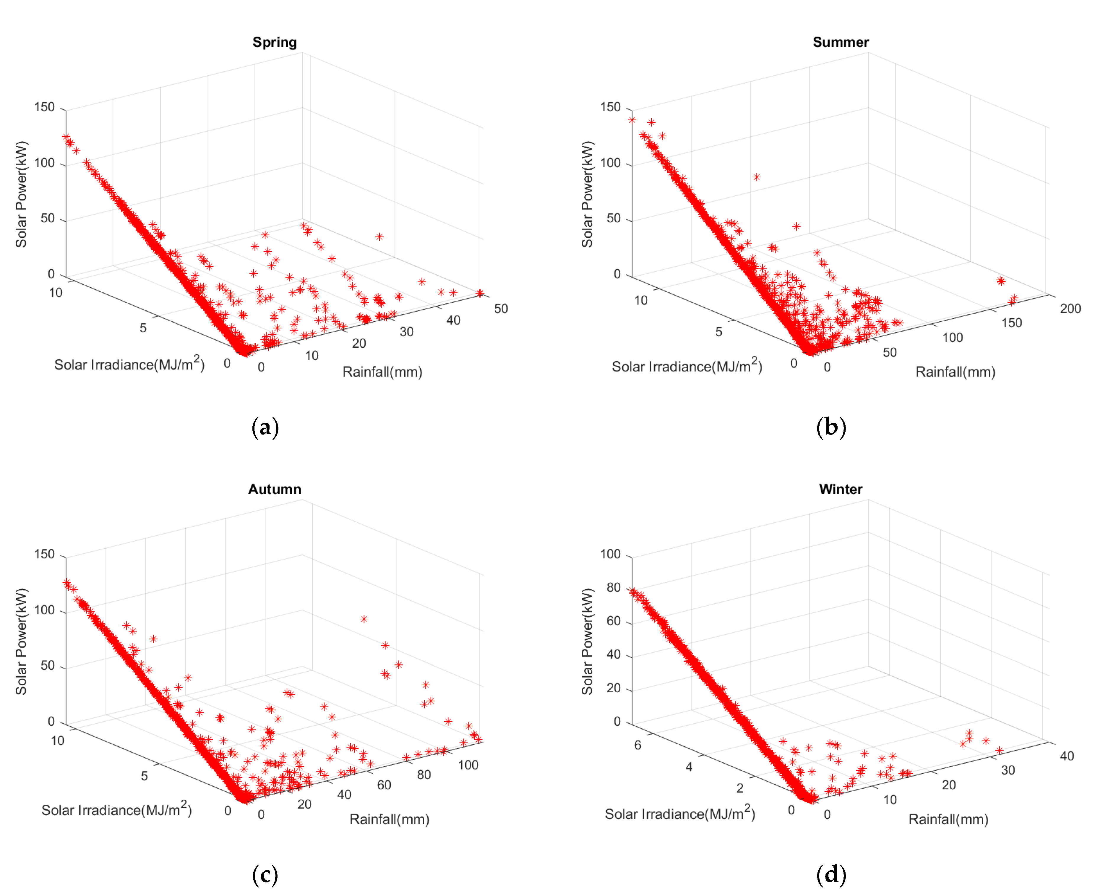
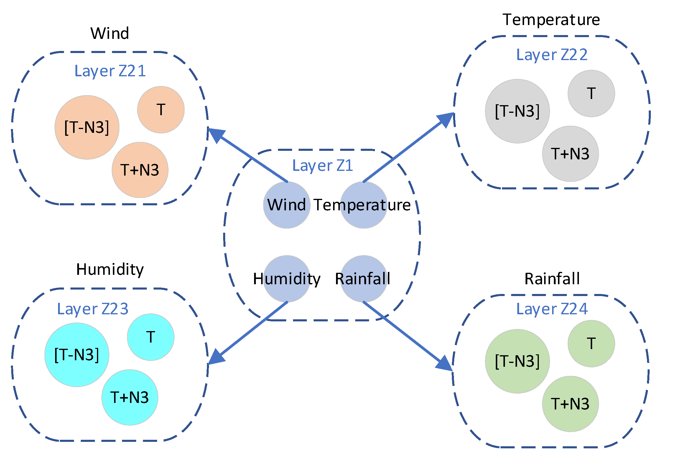
2.1. Weather Clustering
2.1.1. Self-Organizing Map Algorithm Flow
- Step 1: Initialization.
- Step 2: Input example feature vector.
- Step 3: Find the winner neuron.
- Step 4: Adjust the link value vector.
2.1.2. Photovoltaic Power Generation Model
- (1)
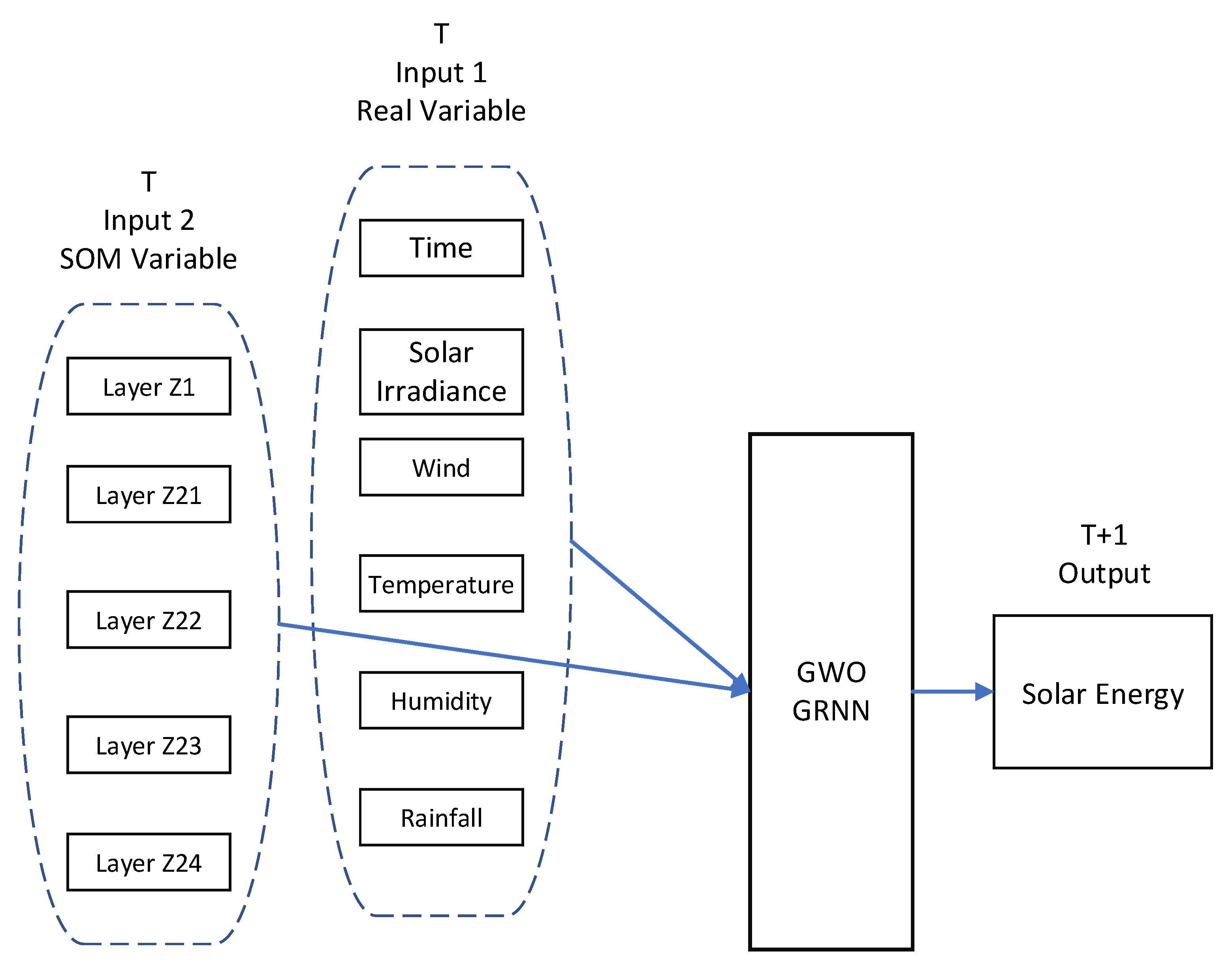
- Input 1 (real variable) represents the actual value (generally the parameter size, weight, and spacing difference of each datum are different).
- (2)
- Input 2 (SOM variable) represents the value of each data group (which can be clearly classified as the Layer Z1 and Layer Z2) and uses Input 1 + Input 2, as shown in Figure 4.
2.2. Performance Evaluation
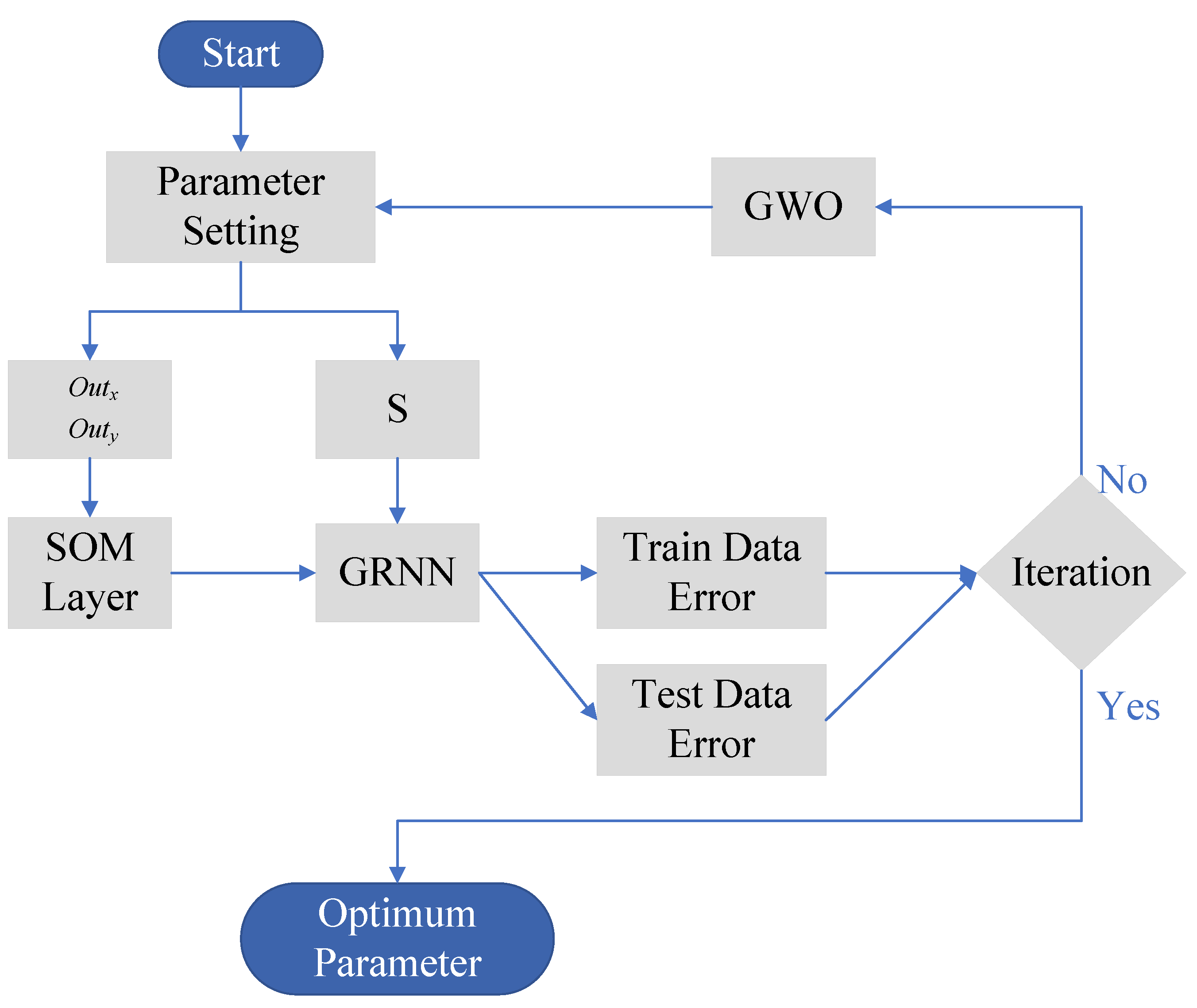
3. Proposed General Regression Neural Network with Grey Wolf Optimization
3.1. Generalized Regression
3.2. Grey Wolf Optimization
4. Numerical Results
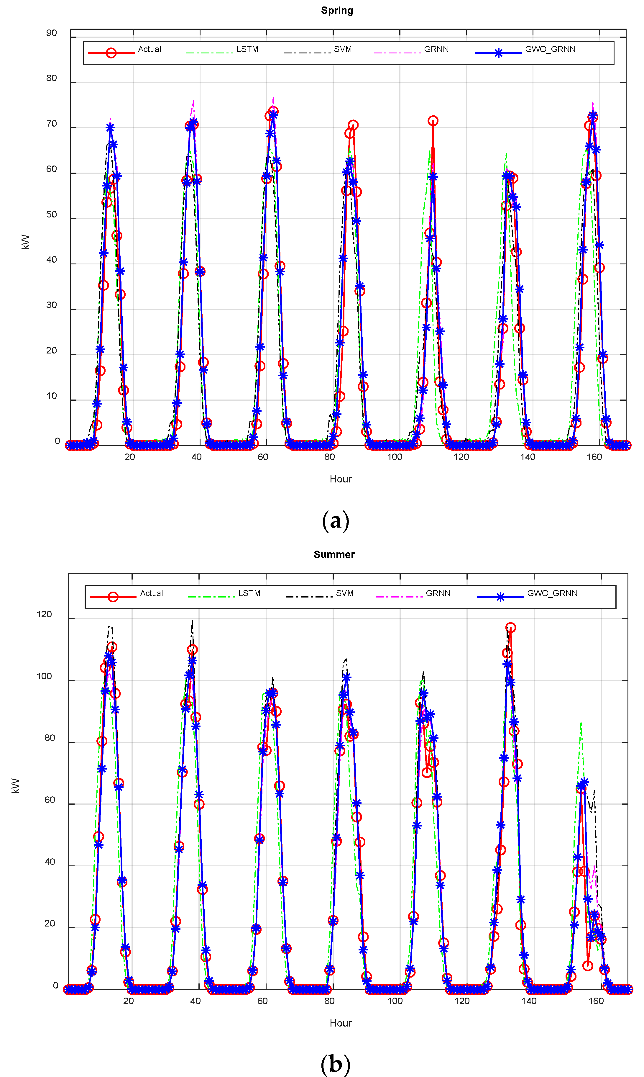
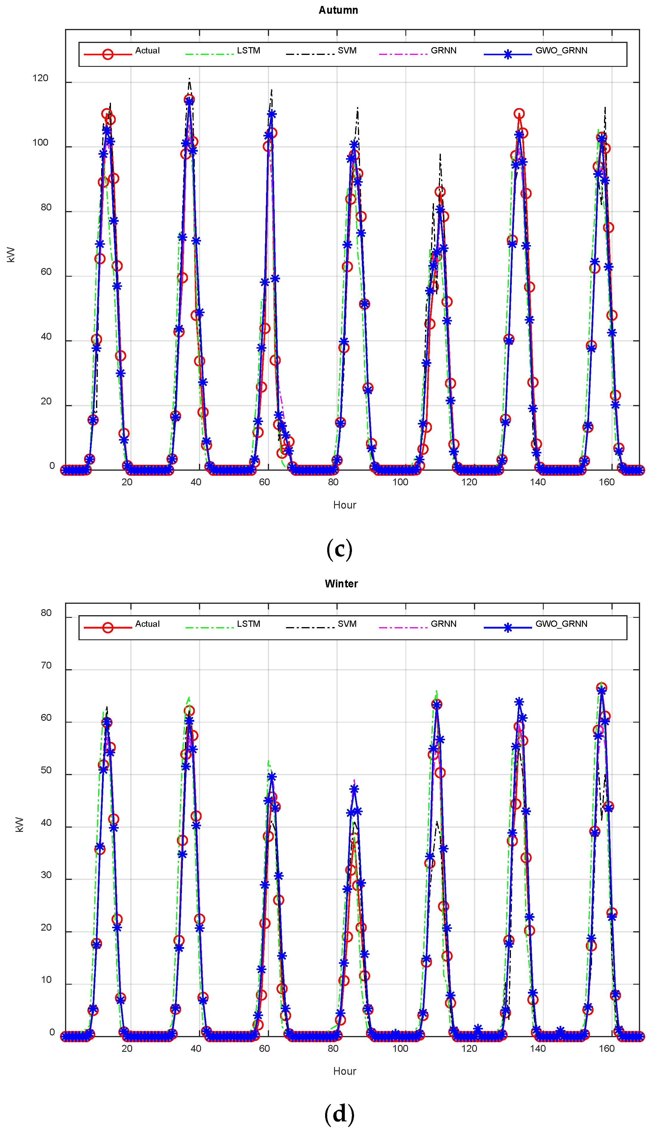
4.1. Short Term Solar Power Forecasting (Hours)
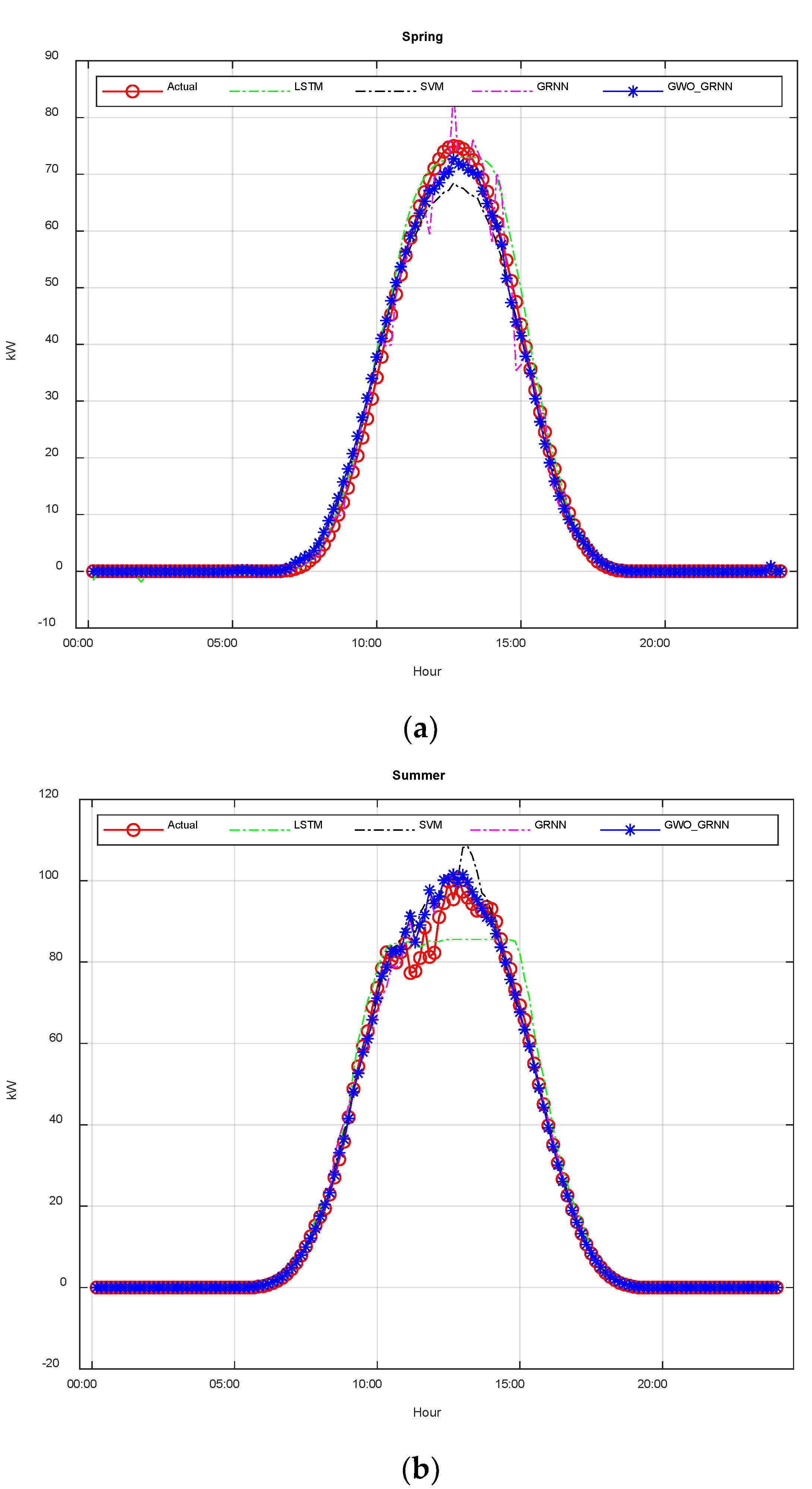
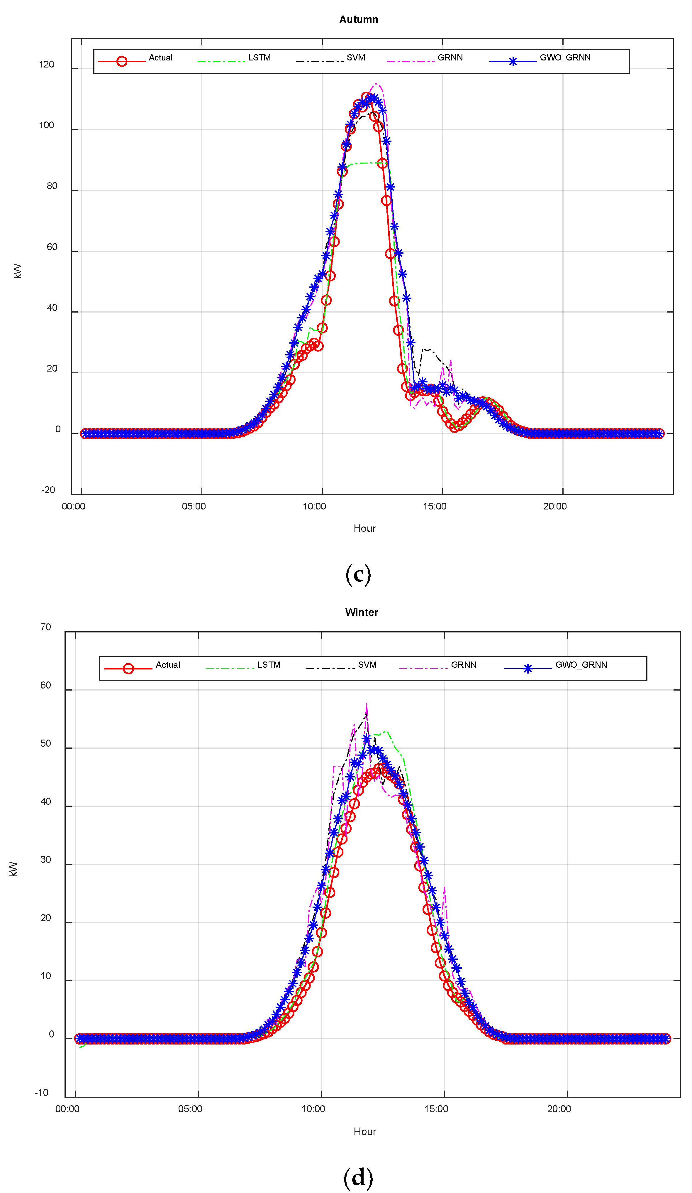
4.2. Ultra-Short-Term Solar Forecasting (10 min)
4.3. Stability and Robustness of the Forecasting Model
5. Discussion
6. Conclusions
Author Contributions
Funding
Institutional Review Board Statement
Informed Consent Statement
Data Availability Statement
Conflicts of Interest
Abbreviations
| PV | Photovoltaic |
| GP | Genetic Programming |
| GMDH | Group Method of Data Handling |
| GRNN | General Regression Neural Network |
| BPNN | Backpropagation Neural Network |
| RBFN | Radial Basis Function Neural Network |
| RNN | Recurrent Neural Networks |
| ANN | Artificial Neural Networks |
| GWO | Grey Wolf Optimization |
| GWO_GRNN | General Regression Neural Network with Grey Wolf Optimization |
| AR | Auto-Regression |
| MA | Moving Average |
| ARMA | Auto-Regression Moving Average |
| ARIMA | Autoregressive Integrated Moving Average |
| SOM | Self-Organizing Map |
| MRE | Mean Relative Error |
| MAE | Mean Absolute Error |
| MBE | Mean Bias Error |
| RMSE | Root Mean Squared Error |
| MAPE | Mean Absolute Percent Error |
| nMBE | Normalized Mean Bias Error |
| R2 | Coefficient of Determination |
| LSTM | Long-Short Term Memory |
| SVM | Support Vector Machine |
Parameters
| The actual power | |
| The predicted power | |
| The average power | |
| Smoothness parameter | |
| Two random vectors | |
| The updated values at iteration | |
| The iteration number | |
| The total number of iterations |
References
- Solarbuzz. Solar Energymarket Growth: Globalmarket Size. 2010. Available online: www.solarbuzz.com/facts-andfigures/markets-growth/market-growth (accessed on 14 February 2011).
- Li, Y.; Su, Y.; Shu, L. An ARMAX Model for Forecasting the power output of a grid connected photovoltaic system. Renew. Energy 2014, 66, 78–89. [Google Scholar] [CrossRef]
- Tao, Y.; Chen, Y. Distributed PV power forecasting using genetic algorithm based neural network approach. In Proceedings of the International Conference Advanced Mechatronic Systems, Kumamoto, Japan, 10–14 August 2014; pp. 557–560. [Google Scholar]
- Wang, S.; Zhang, N.; Zhao, Y.; Zhan, J. Photovoltaic system power forecasting based on combined grey model and BP neural network. In Proceedings of the International Conference Electrical and Control Engineering (ICECE), Yichang, China, 16–18 September 2011; pp. 4623–4626. [Google Scholar]
- Ciabattoni, L.; Ippoliti, G.; Longhi, S.; Cavalletti, M.; Rocchetti, M. Solar irradiation forecasting using RBF networks for PV systems with storage. In Proceedings of the IEEE International Conference Industrial Technology (ICIT), Athens, Greece, 19–21 March 2012; pp. 699–704. [Google Scholar]
- Li, Z.Y.; Zhou, Y.L.; Cheng, C.; Li, Y.; Lai, K.X. Short term photovoltaic power generation forecasting using RBF neural network. In Proceedings of the Chinese Control and Decision Conference (CCDC), Changsha, China, 29 May–2 June 2014; pp. 2758–2763. [Google Scholar]
- Capizzi, G.; Napoli, C.; Bonanno, F. Innovative second-generation wavelets construction with recurrent neural networks for solar radiation forecasting. IEEE Trans. Neural Netw. Learn. Syst. 2012, 23, 1805–1815. [Google Scholar] [CrossRef] [PubMed]
- Kardakos, E.G.; Alexiadis, M.C.; Vagropoulos, S.I.; Simoglou, C.K.; Biskas, P.N.; Bakirtzis, A.G. Application of time series and artificial neural network models in short-term forecasting of PV power generation. In Proceedings of the International Universities Power Engineering Conference (UPEC), Dublin, Ireland, 2–5 September 2013; pp. 1–6. [Google Scholar]
- Li, Y.Z.; Niu, J.C. Forecast of power generation for grid-connected photovoltaic system based on Markov chain. In Proceedings of the Asia-Pacific Power and Energy Engineering Conference (APPEEC), Wuhan, China, 28–30 March 2009; pp. 1–4. [Google Scholar]
- Huang, C.Y.; Tzeng, W.C.; Liu, Y.W.; Wang, P.Y. Forecasting the global photovoltaic market by using the GM(1,1) grey forecasting method. In Proceedings of the IEEE Green Technologies Conference, Baton Rouge, LA, USA, 15–6 April 2011; pp. 1–5. [Google Scholar]
- Haque, A.U.; Nehrir, M.H.; Mandal, P. Solar PV power generation forecast using a hybrid intelligent approach. In Proceedings of the IEEE Power and Energy Society General Meeting, Vancouver, BC, Canada, 21–25 July 2013; pp. 1–5. [Google Scholar]
- Yang, Y.; Dong, L. Short-term PV generation system direct power prediction model on wavelet neural network and weather type clustering. In Proceedings of the International Conference Intelligent Human-Machine Systems and Cybernetics, Hangzhou, China, 26–27 August 2013; pp. 207–211. [Google Scholar]
- Mellit, A.; Hadjarab, A.; Khorissi, N.; Salhi, H. An ANFIS-based forecasting for solar radiation data from sunshine duration and ambient temperature. In Proceedings of the IEEE Power Engineering Society General Meeting, Tampa, FL, USA, 24–28 June 2007; pp. 1–6. [Google Scholar]
- Yang, H.T.; Huang, C.M.; Huang, Y.C.; Pai, Y.S. A weather-based hybrid method for 1-day ahead hourly forecasting of PV power output. IEEE Trans. Sustain. Energy 2014, 5, 917–926. [Google Scholar] [CrossRef]
- Sansa, I.; Missaoui, S.; Boussada, Z.; Bellaaj, N.M.; Ahmed, E.M.; Orabi, M. PV power forecasting using different artificial neural networks strategies. In Proceedings of the IEEE International Green Energy, Long Beach, CA, USA, 24 November 2014; pp. 54–59. [Google Scholar]
- Felix, M.R.; Sina, K.; Stefan, H. Supervised and Semi-Supervised Self-Organizing Maps for Regression and Classification Focusing on Hyperspectral Data. Remote Sens. 2020, 12, 7. [Google Scholar]
- Hsu, S.H.; Hsieh, J.P.A.; Chih, T.C.; Hsu, K.C. A two-stage architecture for stock price forecasting by integrating self-organizing map and support vector regression. Expert Syst. 2009, 36, 7947–7951. [Google Scholar] [CrossRef]
- Alencar, D.B.; Affonso, C.M.; Oliveira, R.C.L.; Rodríguez, J.L.M.; Leite, J.C.; Filho, J.C.R. Different models for forecasting wind power generation: Case study. Energies 2017, 10, 1976. [Google Scholar]
- Chang, X.; Li, W.; Zomaya, A.Y. A Lightweight Short-Term Photovoltaic Prediction for Edge Computing. IEEE Access 2020, 4, 946–955. [Google Scholar] [CrossRef]
- Kenji, N.F.; Anna, D.P.L.; Carlos, R.M. Short-term multinodal load forecasting using a modified general regression neural network. IEEE Trans. Power Deliv. 2011, 26, 2862–2869. [Google Scholar]
- Specht, D.F. Probabilistic neural network for classification, mapping, or associative memory. In Proceedings of the IEEE International Conference Neural Network, San Diego, CA, USA, 24–27 July 1988; pp. 525–532. [Google Scholar]
- Hong, C.M.; Cheng, F.S.; Chen, C.H. Optimal Control for Variable-Speed Wind Generation Systems using General Regression Neural Network. Int. J. Electr. Power Energy Syst. 2014, 60, 14–23. [Google Scholar] [CrossRef]
- Parzen, E. On estimation of a probability density function and mode. Annals. Math. Stat. 1962, 33, 1065–1076. [Google Scholar] [CrossRef]
- Zhang, Y.; Liu, D.; Liu, J.; Xian, Y.; Wang, X. Improved Deep Neural Network for OFDM Signal Recognition Using Hybrid Grey Wolf Optimization. IEEE Access 2020, 8, 133622–133632. [Google Scholar] [CrossRef]
- Majhi, D.; Rao, M.; Sahoo, S.; Dash, S.P.; Mohapatra, D.P. Modified Grey Wolf Optimization(GWO) based Accident Deterrence in Internet of Things (IoT) enabled Mining Industry. In Proceedings of the 2020 International Conference on Computer Science, Engineering and Applications (ICCSEA), Gunupur, India, 13–14 March 2020. [Google Scholar]
- Han, S. Modified Grey-Wolf Algorithm Optimized Fractional-Order Sliding Mode Control for Unknown Manipulators with a Fractional-Order Disturbance Observer. IEEE Access 2020, 8, 18337–18349. [Google Scholar] [CrossRef]
- Taiwan Power Company. Available online: https://www.taipower.com.tw/tc/page.aspx?cchk=b6134cc6-838c-4bb9-b77a-0b0094afd49d&cid=406&mid=206 (accessed on 1 January 2021).
- Taiwan Central Weather Bureau Automatic Weather Station. Available online: http://farmer.iyard.org/ (accessed on 1 January 2021).
- Li, G.; Xie, S.; Wang, B.; Xin, J.; Li, Y.; Du, S. Photovoltaic Power Forecasting with Hybrid Deep Learning Approach. IEEE Access 2020, 8, 175871–175880. [Google Scholar] [CrossRef]
- Hossain, M.S.; Mahmood, H. Short-Term Photovoltaic Power Forecasting Using an LSTM Neural Network and Synthetic Weather Forecast. IEEE Access 2020, 8, 172524–172533. [Google Scholar] [CrossRef]
- Li, G.; Wang, H.; Zhang, S.; Xin, J.; Liu, H. Recurrent Neural Networks Based Photovoltaic Power Forecasting Approach. Energies 2019, 12, 2538. [Google Scholar] [CrossRef]
- Shi, J.; Lee, W.J.; Liu, Y.; Yang, Y.; Wang, P. Forecasting Power Output of Photovoltaic Systems Based on Weather Classification and Support Vector Machines. IEEE Trans. Ind. Appl. 2015, 48, 1064–1069. [Google Scholar] [CrossRef]
- Wang, H.; Yi, H.; Peng, J.; Wang, G.; Liu, Y.; Jiang, H.; Liu, W. Deterministic and probabilistic forecasting of photovoltaic power based on deep convolutional neural network. Energy Convers. Manag. 2017, 153, 409–422. [Google Scholar] [CrossRef]


| Y, D − 3 | Y, D − 2 | Y, D − 1 | Y, D | Y, D + 1 | Y, D + 2 | Y, D + 3 |
| Y − 1, D − 3 | Y − 1, D − 2 | Y − 1, D − 1 | Y − 1, D | Y − 1, D + 1 | Y − 1, D + 2 | Y − 1, D + 3 |
| Y − 2, D − 3 | Y − 2, D − 2 | Y − 2, D − 1 | Y − 2, D | Y − 2, D + 1 | Y − 2, D + 2 | Y − 2, D + 3 |
| Mean Error | Total Data | min | LSTM | SVM | GRNN | GWO_GRNN |
|---|---|---|---|---|---|---|
| MAE (kW) | 4032 | 10 | 1.549 | 1.621 | 1.555 | 1.469 |
| 1344 | 30 | 1.698 | 1.927 | 1.729 | 1.479 | |
| 672 | 60 | 1.838 | 2.138 | 1.767 | 1.518 | |
| 448 | 90 | 1.889 | 2.274 | 1.846 | 1.502 | |
| RMSE (kW) | 4032 | 10 | 3.534 | 3.736 | 3.573 | 3.333 |
| 1344 | 30 | 4.100 | 4.716 | 3.840 | 3.484 | |
| 672 | 60 | 4.356 | 5.154 | 3.844 | 3.533 | |
| 448 | 90 | 4.534 | 5.506 | 4.105 | 3.539 |
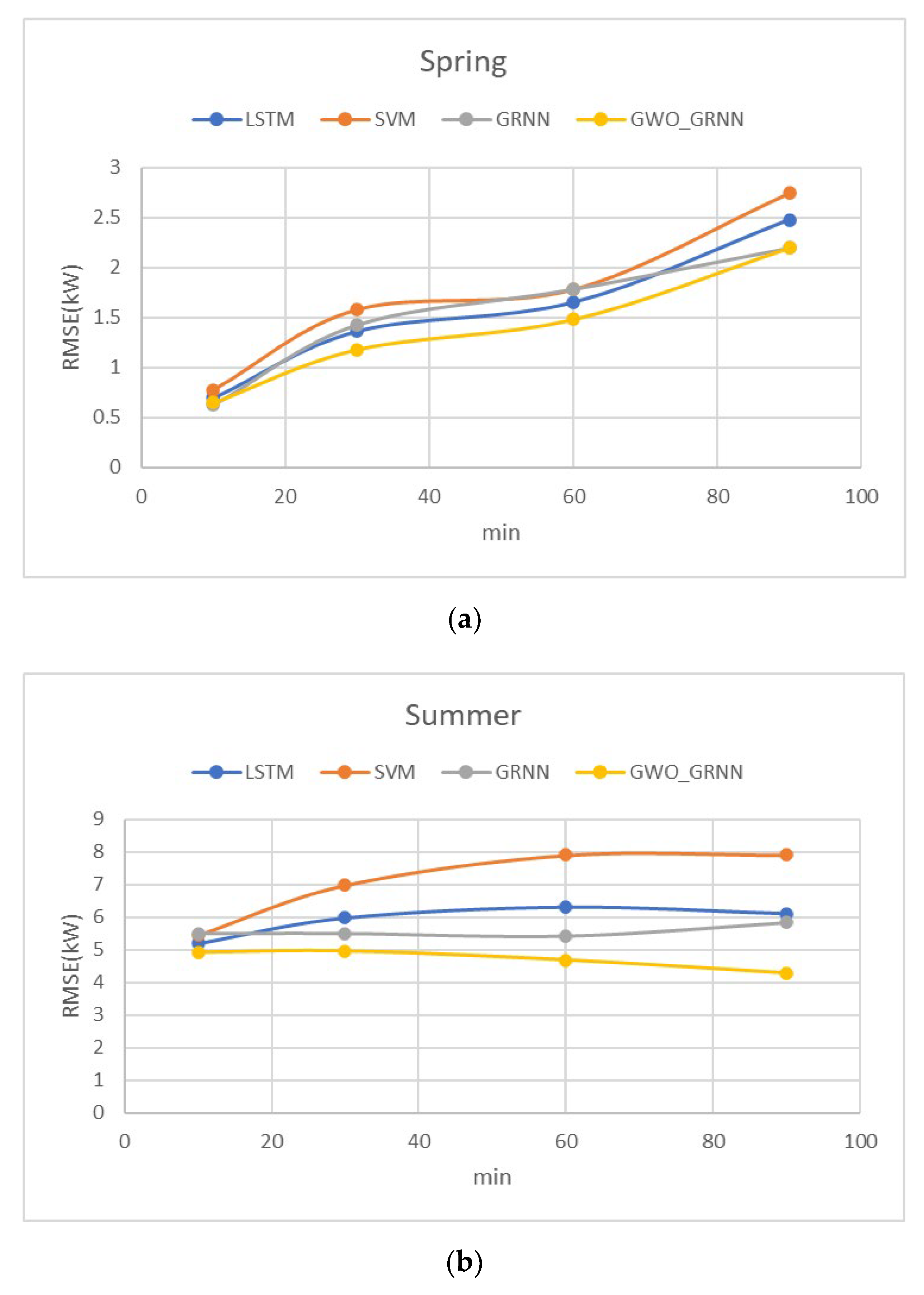
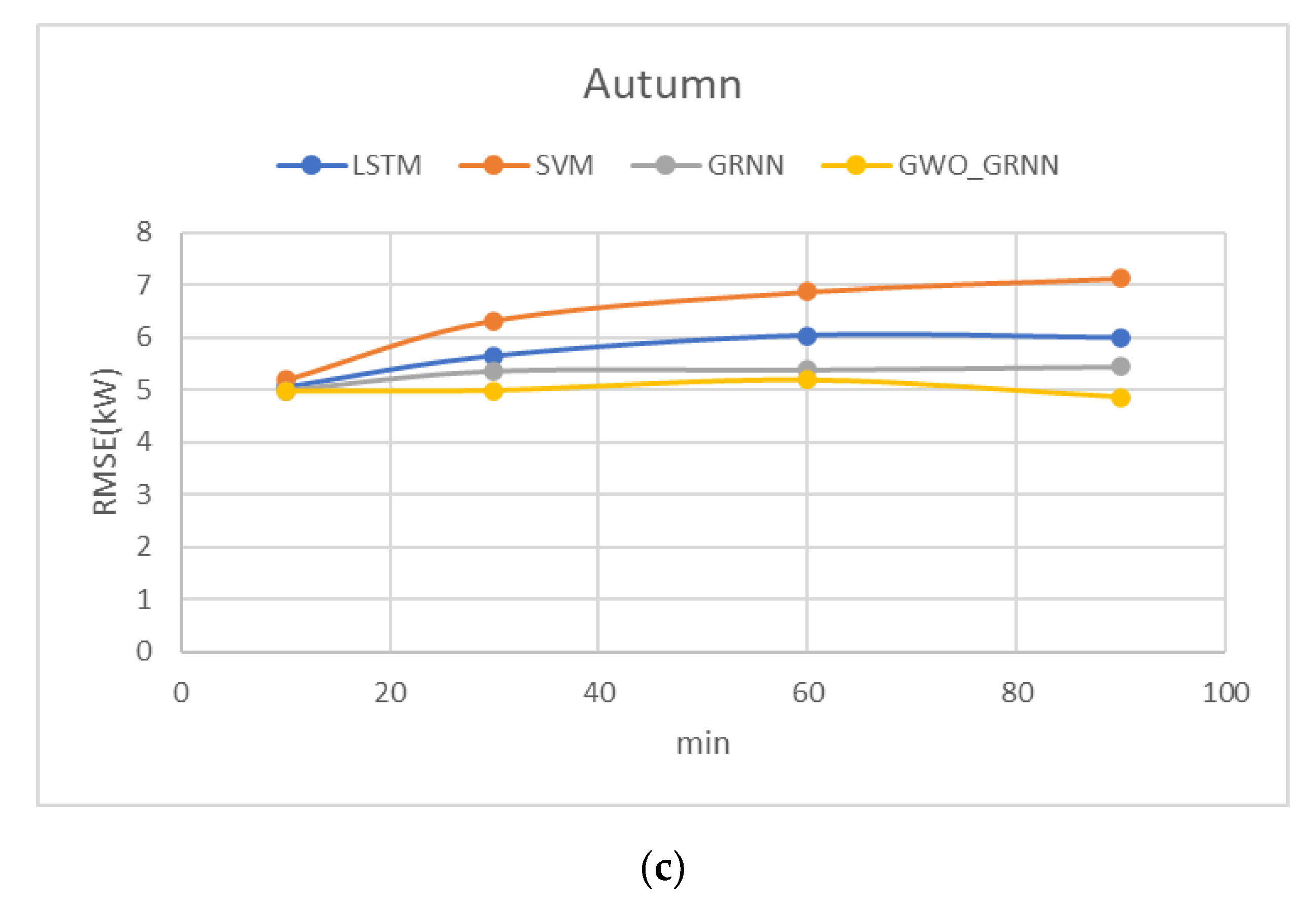
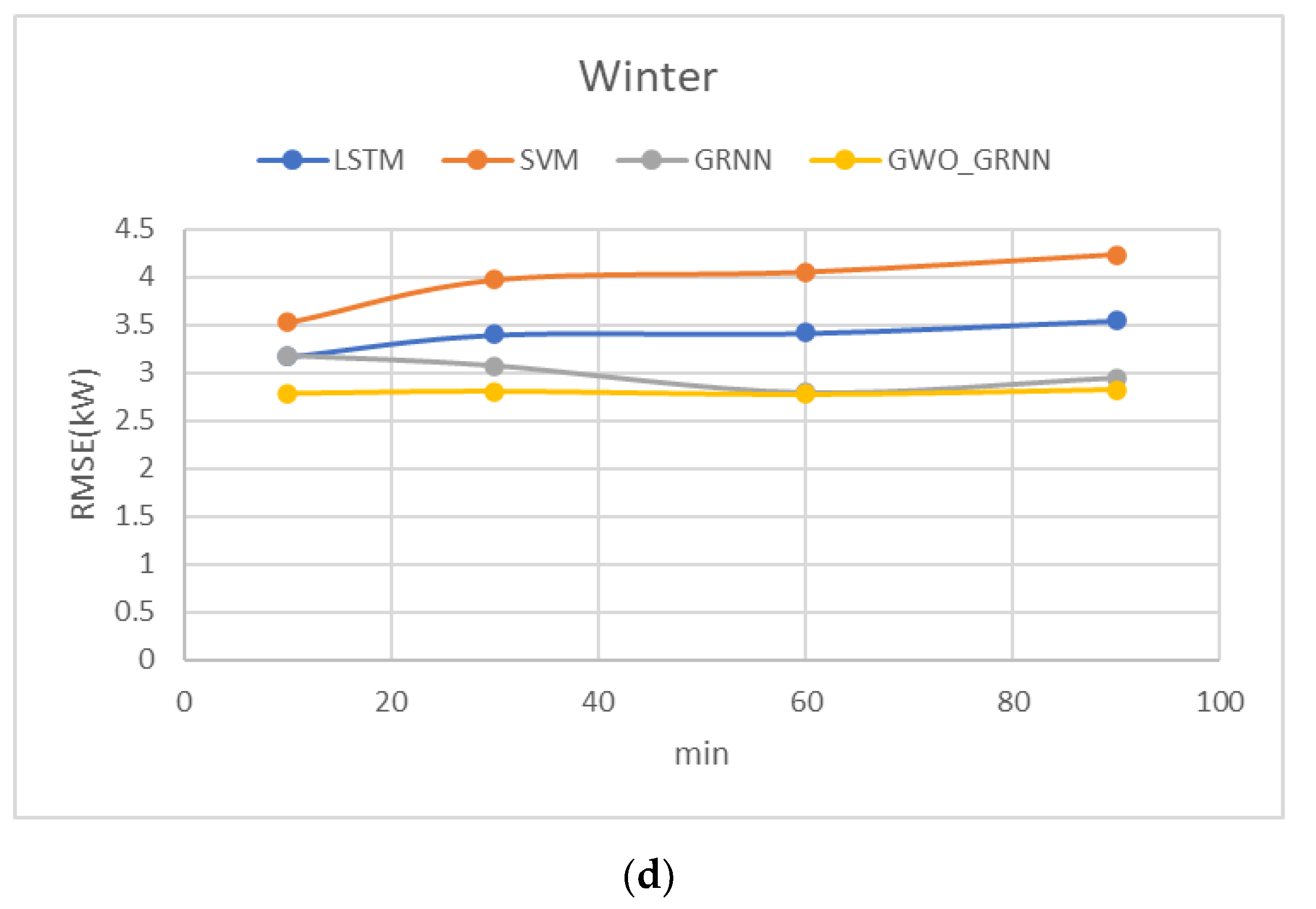
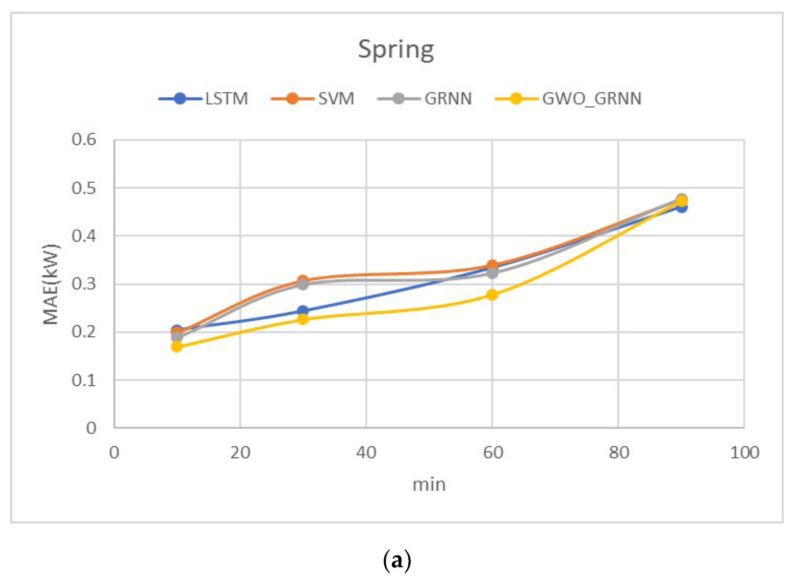
| Seasons | Error | LSTM | SVM | GRNN | GWO_GRNN |
|---|---|---|---|---|---|
| Spring (1 March 2020~7 March 2020) Data 168 | MAE (kW) | 2.0299 | 2.302 | 1.966 | 1.743 |
| RMSE (kW) | 4.041 | 4.557 | 3.889 | 3.558 | |
| MAPE (%) | 0.0177 | 0.033 | 0.023 | 0.011 | |
| MRE (%) | 1.0085 | 1.151 | 0.983 | 0.871 | |
| MBE (kW) nMBE (%) R2 | 0.5506 0.0083 1.0358 | 0.214 0.0090 1.1148 | 1.120 0.0166 1.8870 | 0.929 0.0079 0.9598 | |
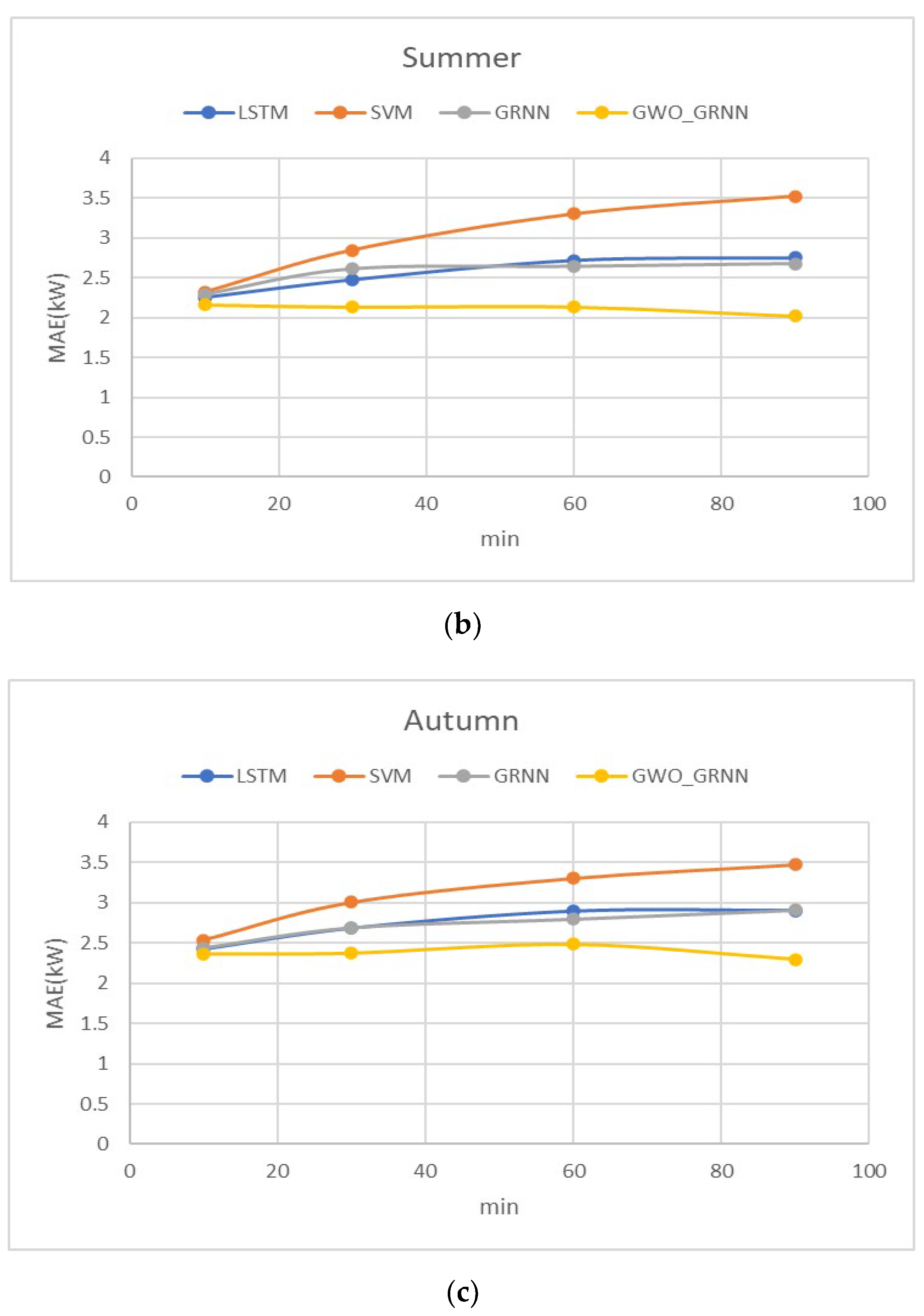
| Summer (1 June 2020~7 June 2020) Data 168 | MAE (kW) | 2.7282 | 3.302 | 2.641 | 2.133 |
| RMSE (kW) | 6.2856 | 7.910 | 5.414 | 4.687 | |
| MAPE (%) | 0.0103 | 0.040 | 0.009 | 0.006 | |
| MRE (%) | 1.365 | 1.651 | 1.321 | 1.067 | |
| MBE (kW) nMBE (%) R2 | 1.5336 0.1052 0.3162 | 2.420 0.1152 1.1776 | 0.473 0.2119 2.0036 | 0.654 0.1004 0.9479 | |
| Autumn (1 September 2020~7 September 2020) Data 168 | MAE (kW) | 2.9177 | 3.304 | 2.795 | 2.489 |
| RMSE (kW) | 6.0528 | 6.871 | 5.384 | 5.190 | |
| MAPE (%) | 0.031 | 0.018 | 0.028 | 0.005 | |
| MRE (%) | 1.4345 | 1.652 | 1.398 | 1.245 | |
| MBE (kW) nMBE (%) R2 | 0.6653 0.0564 1.8784 | 1.028 0.0509 1.1051 | −0.337 0.0982 2.1548 | 0.346 0.0464 0.9600 | |
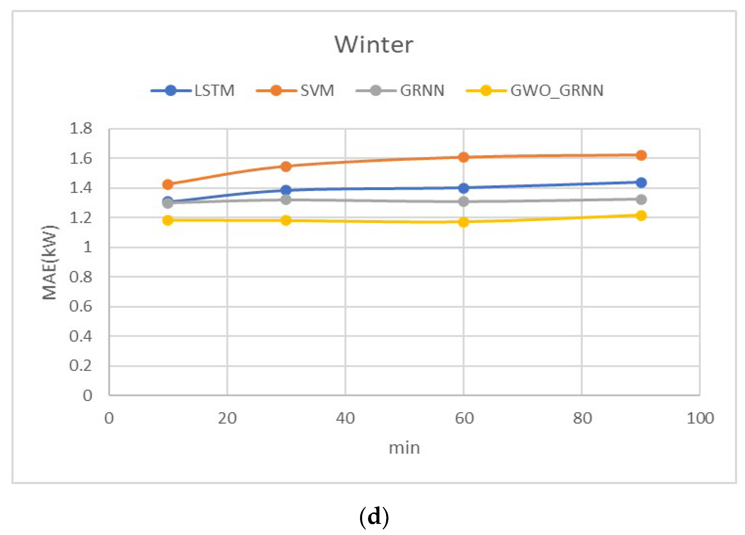
| Winter (1 December 2020~7 December 2020) Data 168 | MAE (kW) | 1.408 | 1.607 | 1.309 | 1.172 |
| RMSE (kW) | 3.4116 | 4.054 | 2.794 | 2.776 | |
| MAPE (%) | 0.04 | 0.050 | 0.003 | 0.027 | |
| MRE (%) | 0.7189 | 0.803 | 0.655 | 0.586 | |
| MBE (kW) nMBE (%) R2 | 0.1171 −0.0958 1.1328 | −0.645 −0.0656 1.0164 | 0.385 −0.1292 1.9329 | 0.863 −0.0586 0.9523 | |
| Average | MAE (kW) | 2.2709 | 2.6287 | 2.177 | 1.884 |
| RMSE (kW) | 4.9477 | 5.848 | 4.370 | 4.052 | |
| MAPE (%) | 0.0247 | 0.0352 | 0.015 | 0.012 | |
| MRE (%) | 1.1317 | 1.3142 | 1.089 | 0.942 | |
| MBE (kW) nMBE (%) R2 | 0.7166 0.0185 1.0908 | 0.7542 0.0273 1.1034 | 0.410 0.049 1.994 | 0.698 0.024 0.955 |
| Mean Error | LSTM | SVM | GRNN | GWO_GRNN |
|---|---|---|---|---|
| MAE (kW) | 2.271 | 2.134 | 2.041 | 1.907 |
| RMSE (kW) | 4.948 | 4.652 | 4.315 | 4.101 |
| MAPE (%) | 0.025 | 0.002 | 0.002 | 0.002 |
| MRE (%) | 1.132 | 1.067 | 1.021 | 0.953 |
| MBE (kW) | 0.717 | 0.617 | 0.518 | 0.653 |
| nMBE (%) | 0.0185 | 0.0274 | 0.0494 | 0.0240 |
| R2 (%) | 1.0908 | 1.1035 | 1.9946 | 0.9550 |
Publisher’s Note: MDPI stays neutral with regard to jurisdictional claims in published maps and institutional affiliations. |
© 2022 by the authors. Licensee MDPI, Basel, Switzerland. This article is an open access article distributed under the terms and conditions of the Creative Commons Attribution (CC BY) license (https://creativecommons.org/licenses/by/4.0/).
Share and Cite
Tu, C.-S.; Tsai, W.-C.; Hong, C.-M.; Lin, W.-M. Short-Term Solar Power Forecasting via General Regression Neural Network with Grey Wolf Optimization. Energies 2022, 15, 6624. https://doi.org/10.3390/en15186624
Tu C-S, Tsai W-C, Hong C-M, Lin W-M. Short-Term Solar Power Forecasting via General Regression Neural Network with Grey Wolf Optimization. Energies. 2022; 15(18):6624. https://doi.org/10.3390/en15186624
Chicago/Turabian StyleTu, Chia-Sheng, Wen-Chang Tsai, Chih-Ming Hong, and Whei-Min Lin. 2022. "Short-Term Solar Power Forecasting via General Regression Neural Network with Grey Wolf Optimization" Energies 15, no. 18: 6624. https://doi.org/10.3390/en15186624