Research on the Characteristics of the Solid–Liquid Two-Phase Flow Field of a Submersible Mixer Based on CFD-DEM

Abstract

Submersible mixers are widely used in the sewage treatment process in various fields, such as agriculture and industry. They are mainly responsible for pushing flow and mixing activated sludge particles in a pool. Based on the CFD-DEM coupling method under the Euler–Lagrange framework, the solid–liquid two-phase flow of a submersible mixer was simulated in this paper, and the motion characteristics and distribution laws of particles in the pool were studied in axial, horizontal, and lateral directions, respectively. An evaluation method of distribution uniformity was proposed to analyze the velocity distribution of the flow field, the velocity distribution of particles, and the mixing uniformity of particles. The results show that the movement process of activated sludge particles in the pool can be roughly divided into three stages: the horizontal development stage, absorption–injection stage, and reflux-mixing stage, in which the reflux-mixing stage is the main stage for the uniform distribution of particles in the whole flow field. Particle accumulation occurs mainly in the dead zones of the flow field. Distribution of particles in the axial direction has the most homogeneous extent. Vortices can be generated near pool walls, causing accumulation of particles. This method can be a good guide for engineering practice.

1. Introduction

With the growing economy in China and the increasing discharge of sewage, sewage treatment has become an extremely significant issue. The activated sludge method is currently one of the major technologies for treating sewage, and it is a biological treatment method of the push-flow type. This technology mixes wastewater with activated sludge and aeration to break down the organic pollutants in the wastewater. The process requires the activated sludge to be in suspension in a pool [1].

The primary function of a submersible mixer is to keep the flow of wastewater inside the pool and to prevent the sedimentation of the activated sludge, which is widely used in various wastewater treatment scenarios. The impeller of the submersible mixer rotates under the drive of the motor to stir liquid and to generate rotating jets, which uses the shear layer along the surface of jets to mix and applies a large volume flow pattern to achieve the stirring and pushing transport of fluid. Research on the submersible mixer and its flow field characteristics is of great significance [2]. Xu et al. compared the flow field distribution in the pool under two cases of a submersible mixer installation depth of 3 m and 5.72 m, using numerical simulation. It was found that the installation position close to the bottom of the pool can form a high-speed flow area on the bottom surface of the pool, which contributes to stop the deposition of solid particles [3]. Xu et al. found that the blade gap has a certain influence on the mixing effect of submersible mixers by comparing the velocity flow field under different blade gaps, and the effective mixing ratio first increases and then decreases with the increase of the blade gap [4]. Ren et al. studied the flow field under the three models of blade placement angles of −4°, 0°, and 4° and found that the effective mixing area increased with the increasing blade placement angle, and the mixing effect was better [5].

At present, domestic scholars and those from abroad have conducted numerous studies on the jet characteristics of a submersible mixer in clear water and in the flow field inside a pool, while relatively fewer studies have been carried out on the two-phase flow of sludge-wastewater.

There are two major approaches to the study of solid–liquid two-phase flow: Euler–Euler model and Euler–Lagrange model. The Euler–Euler model treats solid and liquid phases as a continuous medium that mixes with each other, and puts both solid and liquid phases into a Euler coordinate system for solution [6]. Currently, the mixture model is the most popular model, which treats sludge and wastewater as a mixed continuous medium. Jin et al. compared the flow field of clear water flow and the flow field of a sewage–sludge two-phase mixed flow based on the mixture model and found that the sedimentation was obvious at the bottom of the pool and underneath the mixer [7]. Tian et al. studied the three-dimensional two-phase flow field of a submersible mixer using the mixture model. It was found that the number of particles in dead zones at the bottom of the pool was significantly higher than the number of particles in dead zones of other locations [8]. The above studies have greatly contributed to the research on the solid–liquid two-phase flow of submersible mixers. However, the phenomena of particle rotation, collision, aggregation, and bonding cannot be truly reflected; the collision and wear of particles on the impeller cannot be reliably simulated; and the influence of parameters, such as the shape and size of particles on their motion, cannot be accurately studied. To more accurately analyze the motion of particles in solid–liquid two-phase flows, the numerical simulation method based on coupled CFD-DEM is now widely applied. The DEM model is implemented within Lagrange architecture, and it was created by Cundall [9]. The model uses the Lagrange phase model to define particles and introduces interparticle forces in the equations of motion, which enables a more accurate analysis of the motion of particles in solid–liquid two-phase flows. The model uses the Lagrange phase model to define particles and introduces inter-particle forces in the equation of motion, which can trace the complex motion of particle clusters and visualize the motion of solid-phase particles, enabling more accurate studies of fluid-particle interaction laws. Li et al. simulated the solid–liquid two-phase flow field in the pump by CFD-DEM method and analyzed the motion characteristics of particles under different working conditions [10]. Zhou et al. studied the effect of particle size distribution on the pressure drop and flow field of pipeline transportation by CFD-DEM coupling method [11]. Xia et al. studied the motion of particles and abrasion phenomena in mixed-flow pumps based on the coupled CFD-DEM method with different particle shapes and particle concentrations [12]. Zhao et al. investigated the effects of rotational speed, paddle diameter, blade inclination, and other factors on the mixing effect of multiphase flow in a mixing system using the coupled CFD-DEM method [13].

This paper investigated the distribution and movement laws of activated sludge particles in the pool under the action of a submersible mixer based on the coupled CFD-DEM numerical simulation method. The influence of sewage on particle motion and the interaction between particle and particle and between particle and wall were considered, and the distribution laws of particles in axial, horizontal, and vertical directions were systematically analyzed.

2. Calculation Model

2.1. Physical Model

Submersible mixer models are usually simplified in numerical simulations, using impellers instead. The calculation model of this paper is a submersible mixer for a sewage station. The impeller diameter is 315 mm; the hub diameter is 105 mm; and the impeller rotational speed is 1600 rpm. The water pool model is a small pool of this sewage station. The size of the pool is L × W × H = 5 m × 3 m × 2 m. The submersible mixer is installed parallel to the bottom of the pool, and the arrangement is shown in Figure 1.

2.2. Mathematical Model

2.2.1. Continuous Phase Mathematical Model

The controlling equation for fluid is as follows:

$$\frac{\partial }{\partial t}\left({\alpha }_f{\rho }_f\right)+\nabla \cdot \left({\alpha }_f{\rho }_f{\mathit{v}}_{\mathit{f}}\right)=0$$

(1)

$$\frac{\partial }{\partial t}\left({\alpha }_f{\rho }_f{\mathit{v}}_{\mathit{f}}\right)+\nabla \cdot \left({\alpha }_f{\rho }_f{\mathit{v}}_{\mathit{f}}{\mathit{v}}_{\mathit{f}}\right)=-{\alpha }_f\nabla p+{\mu }_f{\alpha }_f{\nabla }^2{\mathit{v}}_{\mathit{f}}+{\alpha }_f{\rho }_{f}g+F$$

(2)

where ${\rho }_f$ is the density of fluid, ${\alpha }_f$ is the volume fraction of fluid, ${\mathit{v}}_{\mathit{f}}$ is the velocity vector of fluid, $p$ is the pressure, ${\mu }_f$ is the dynamic viscosity of fluid, $g$ is the acceleration of gravity, and $F$ is the external volume force.

The turbulence model used in this paper is the standard $k-\epsilon$ model, which uses the turbulent kinetic energy $k$ equation and the turbulent dissipation rate $\epsilon$ equation to close time-averaged equations.

2.2.2. DEM Mathematical Model

The discrete phase is solved using Newton’s second law and the law of conservation of angular momentum with the following equations [14]:

$$m_p\frac{d{v}_p}{dt}=F_s+F_b$$

(3)

$$I_p\frac{d{\omega }_p}{dt}=M_b+M_c$$

(4)

where $m_p$ is the particle mass, $v_p$ is the instantaneous particle velocity, $F_s$ is the combined force of forces acting on particle surface, and $F_b$ is the combined force of volume forces, $M_d$ is the drag torque, and $M_c$ is the contact torque.

$$F_s=F_{drag}+F_p+F_{vm}$$

(5)

$$F_b=F_g+F_{LR}+F_{LS}+F_c$$

(6)

$F_{drag}$ is the drag force of the continuous relative discrete phase, and drag coefficient $C_d$ uses the Schilier–Naumann [15] correction model; they are defined as follows:

$$F_{drag}=\frac{1}{2}{C}_d{\rho }_f{A}_p\left|v_f-v_p\right|\left(v_f-v_p\right)$$

(7)

$$C_d=\{\begin{array}{c}\frac{24}{{\mathrm{Re}}_p}\left(1+0.15{\mathrm{Re}}_p^{0.687}\right)R{\mathrm{e}}_p⩽{10}^3\\ 0.44R{\mathrm{e}}_p>{10}^3\end{array}$$

(8)

$${\mathrm{Re}}_p=\frac{{\rho }_f\left|v_f-v_p\right|D_p}{{\mu }_f}$$

(9)

where ${\mathrm{Re}}_p$ is the particle Reynolds number, $D_p$ is the particle diameter, and ${\mu }_f$ is the dynamic viscosity.

$F_p$ is the pressure gradient force, defined as follows:

$$F_p=-V_p\nabla p_{static}$$

(10)

where $V_p$ is the particle volume and $\nabla p_{static}$ is the gradient of the static pressure in continuous phase.

$F_{vm}$ is the virtual mass force, defined as follows:

$$F_{vm}=C_{vm}{\rho }_p{V}_p\left(\frac{Dv}{Dt}-\frac{d{v}_p}{dt}\right)$$

(11)

where $C_{vm}$ is the virtual mass fraction, and, in this paper, $C_{vm}$ is 0.5 and D/Dt is the material derivative.

$F_g$ is the gravitational force of the particle, defined as follows:

$$F_g=m_{p}g$$

(12)

$F_{LR}$ is the particle rotational lift force, which is the lift from counterflow to downflow due to the difference in pressure between the two sides caused by the particle rotation [16], defined as follows:

$$F_{LR}=\frac{\rho \pi }{8}{D}_p^2{C}_{LR}\left|{\upsilon }_f-{\upsilon }_p\right|\frac{\Omega \left(v_f-v_p\right)}{\left|\Omega \right|}$$

(13)

where $\Omega$ is the angular velocity of the particle relative to the fluid and $C_{LR}$ is the rotational lift coefficient, defined as follows:

$$C_{LR}=0.45+\left(\frac{{\mathrm{Re}}_R}{{\mathrm{Re}}_p}-0.45\right)e^{-0.5684{\mathrm{Re}}_R^{0.4}{\mathrm{Re}}_p^{0.3}}$$

(14)

$F_{LS}$ is the particle shear lift force, defined as follows:

$$F_{LS}=C_{LS}\frac{\rho \pi }{8}{D}_p^3\left(v_f-v_p\right)\omega$$

(15)

where $\omega$ is the rotation of fluid velocity, $C_{LS}$ is the shear lift coefficient, given by Saffman [17], defined as follows:

$$C_{LS}=\frac{4.1126}{{\mathrm{Re}}_S^{0.5}}$$

(16)

$F_c$ is the contact force, which indicates the interaction between particles and between particles and walls. In this paper, the Hertz–Mindlin no-slip contact model is chosen, defined as follows [12]:

$$F_c=F_{cn}+F_{ct}$$

(17)

where $F_{cn}$ and $F_{ct}$ are normal and tangential contact forces, respectively, defined as follows:

$$F_{cn}=1.5\frac{Y}{1-{\mu }^2}\sqrt{R_{ab}}\sqrt{u_n^3}$$

(18)

$$F_{ct}=12\left(G_{ab}\sqrt{R_{ab}{u}_n}\right)\sqrt{u_t^3}$$

(19)

where $Y$ is the equivalent modulus of elasticity, $\mu$ is the Poisson’s ratio, $R_{ab}$ is the equivalent contact radius, $u_n$ is the normal displacement, $u_t$ is the tangential displacement, and $G_{ab}$ is the equivalent shear modulus.

3. Numerical Calculation

3.1. Meshing

Due to the large amount of computation based on CFD-DEM coupling, it is necessary to minimize the number of meshes and improve mesh quality. In this paper, the commercial software STARCCM+ is chosen for the automatic mesh generation. Hexahedral meshes are generated in the pool computational region, and the bottom and walls of the pool are encrypted using prismatic layer meshes. The interface between pool and impeller is encrypted with surface meshes. Polyhedral meshes are generated in the impeller computational region. For the numerical calculation of mixer flow field, polyhedral mesh can effectively improve the convergence speed and ensure the computational accuracy [18,19]. Figure 2 shows the meshing of the pool and impeller. The mesh quality of the pool is above 0.95 and that of the impeller is above 0.2.

Five sets of mesh models are established, which are 320,438, 621,211, 1,542,649, 2,186,086 and 4,030,726. The hydraulic thrust and torque are the external characteristic parameters of the submersible mixer impeller, and the mesh independence validation can be performed by comparing the deviation of the hydraulic thrust and torque from the actual model with different mesh quantities. The simulation result of mesh independence verification is as

Table 1. Mesh independence verification.

Serial Number	Mesh Number	Torque [N·m]	Hydraulic Thrust [N]	Torque Deviation [%]	Hydraulic Thrust Deviation [%]
1	320,438	99.8	2056.6	8.26	9.88
2	621,211	105.3	2209.3	3.21	3.19
3	1,542,649	108.3	2279.5	0.46	0.11
4	2,186,086	108.6	2280.4	0.18	0.07
5	4,030,726	108.9	2283.2	0.09	0.05

. It can be seen from Table 1 that after the mesh number reaches 1542649, the numerically simulated torque and water thrust tend to stabilize and deviate less from the actual model. Considering the computational accuracy and computational resources, the third set of mesh was chosen as the object of simulation in this paper.

3.2. Boundary Conditions and Initial Conditions

To increase the convergence rate of the flow field in a single time step, the free surface of the pool is set by the rigid-lid assumption. To prevent particles from escaping from the free surface, it is set to phase impermeable.

The continuous phase is solved by the MRF method, the blade is set to rotational domain, and the intersection of impeller and pool is set to interface. The rest of the walls are set to no-slip wall, and the wall specification is smooth. Considering the interaction between walls and particles, walls are specified as DEM mode.

3.3. Other Settings

The standard $\kappa -\epsilon$ turbulence model is selected for the turbulence model, and the wall treatment is high y+ wall treatment with y+ > 30, and the convergence residual of continuity is set to 10⁻⁴.

The MLSS concentration is 1500 mg/L, the diameter of particles is 6 mm, and the number of particles is roughly 396,500. An injector is set near the water surface, and particles are injected vertically downward with a jet flow rate of 99,125 particles/s and a jet time of 4 s. The initial velocity of particles is set to 0.25 m/s. Particles are activated sludge particles with a density of 1004 kg/m³, Poisson’s ratio of 0.45, and Young’s modulus of 0.21 Mpa.

The Hertz–Mindlin no-slip contact model is chosen for the interphase interaction between particles and between particles and walls. DEM time step is set to 0.000497 s; the continuous phase time step is set to 0.00497 s. The second-order implicit unsteady solver is used to solve the problem, and the total solution time is 34.1 s.

4. Result and Discussion

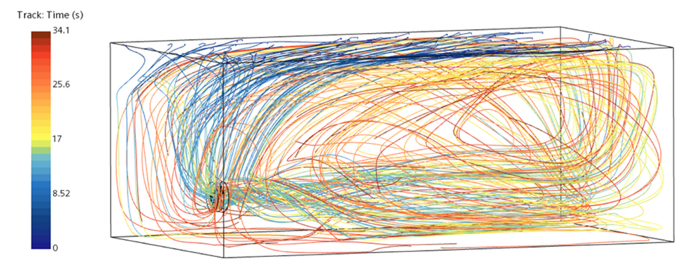
4.1. Distribution of Pool Flow Field

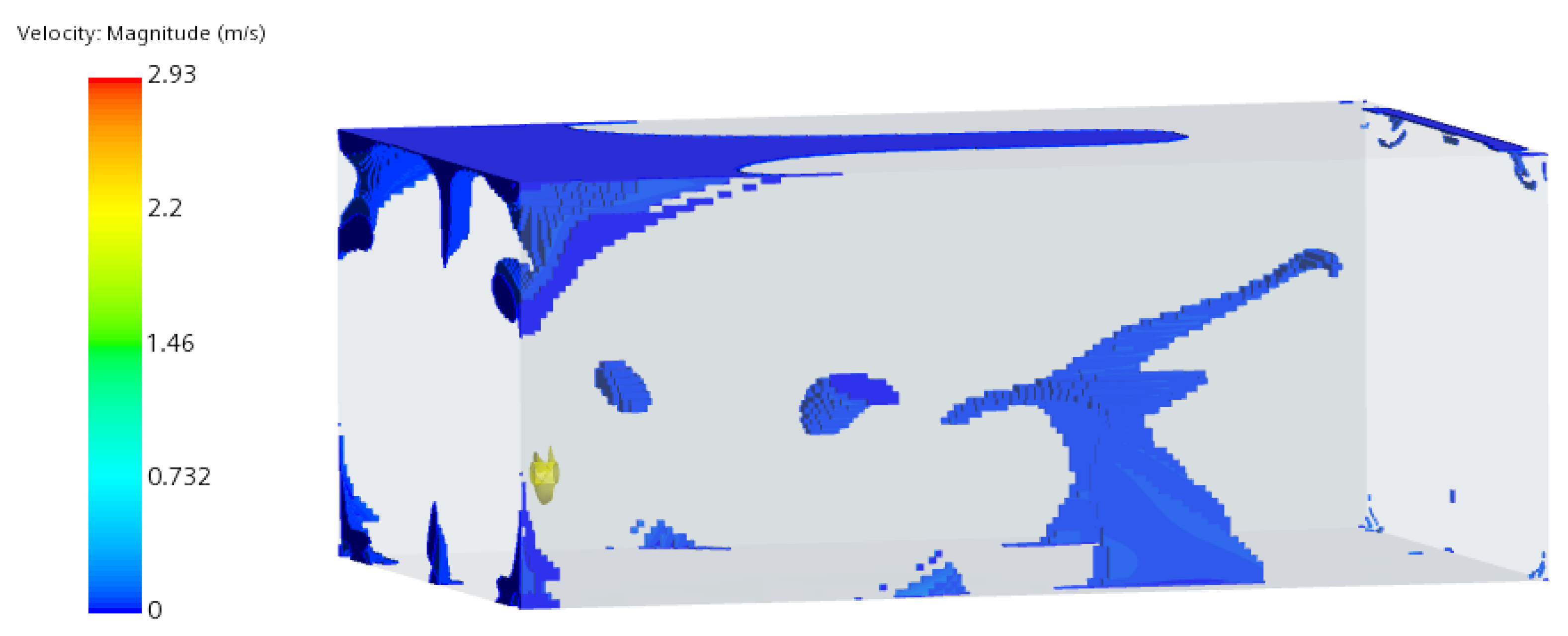
4.1.1. Distribution of Velocity and Turbulent Kinetic Energy Distribution

In the solid–liquid mixing flow field of submersible agitation, the movement of particles is strongly affected by the flow field as the density of activated sludge is similar to that of sewage, and the turbulent kinetic energy and velocity of the flow field can characterize the mixing capacity of the flow field to a certain extent, which is the key factor affecting the distribution of activated sludge inside the pool.

The maximum value of turbulent energy inside the pool is 8.06 J/kg, located near the tip of the impeller, and the minimum value of turbulent energy is 0.0021 J/kg, located at the junction of the walls of the pool. As shown in Figure 3, with the approach of the plane to the Y = −1.3 plane, the core area of velocity and turbulent kinetic energy gradually moves forward along the Z-axis. In submerged mixing flow field, the turbulent kinetic energy is relatively large where the velocity is large. However, a part of the downstream area of the pool exists where the velocity is large and the turbulent kinetic energy is low. This is attributed to the fact that after the jet hits the wall, part of the jet flows back along the wall of the pool, and the turbulence intensity of the fluid in this part is weak, similar to the state of laminar flow. However, overall, the turbulent kinetic energy is greatly affected by the flow velocity, so the following mainly analyzes the velocity flow field.

Figure 4 and Figure 5 are a velocity streamline diagram of the full flow field and the velocity contour of different axial sections. The development process and trajectories of the flow field in the stirred flow field can be seen from diagrams. It can be seen that after being sucked in by the submersible mixer, the fluid is ejected in the form of a rotating jet. After the jet impacts the wall, it disperses into multiple streams of water and returns to the impeller of the mixer, and it can be seen that the radius of radial disturbance gradually increases and the velocity intensity gradually decreases with the development of the jet.

4.1.2. Uniformity of Velocity Distribution

For the velocity distribution of the flow field, Zhang et al. proposed to evaluate the mixing effect of the submersible mixer by using the effective mixing domain method, i.e., the hydraulic performance of the submersible mixer is judged by calculating the effective mixing (≥0.1 m/s) volume of the water body pushing the flow mixing [20]. The effective mixing volume of the flow field in this paper was 28.46 m³, accounting for 94.8% of the total volume.

The effective mixing domain method can well evaluate the mixing performance of the submersible mixer but is unable to evaluate the velocity distribution of the flow field inside the pool. For solid–liquid two-phase flow, the velocity distribution in the flow field is extremely crucial to ensure the homogeneous distribution of activated sludge in the pool. In this paper, we proposed a method for evaluating the velocity distribution of the submersible mixing flow field based on the evaluation method of Herman for the velocity distribution in the cross-section, i.e., the velocity uniformity method [21]. This method divides the flow field into several regions, statistics the average velocity within each region, and compares its variability with the average velocity of the full flow field. The equation is as follows.

$${\mathsf{\Upsilon }}_{\upsilon }=1-\frac{{\displaystyle {\displaystyle \sum }_c}\left|{\overline{\upsilon }}_c-\overline{\upsilon }\right|V_c}{2\left|\overline{\upsilon }\right|{\displaystyle \underset{c}{{{\displaystyle \sum }}^{ }}}{V}_c}$$

(20)

where ${\overline{\upsilon }}_c$ is the average velocity of the regional flow field, $\overline{\upsilon }$ is the average velocity of the full flow field, and $V_c$ is the volume of the region. Theoretically, this result is more accurate with more zones. The value of ${\mathsf{\Upsilon }}_{\upsilon }$ is larger, indicating that the velocity distribution of the flow field is more uniform, and the maximum value is 1.

The average velocity of the flow field in this paper is 0.497 m/s, which meets the requirements of the submersible mixer for a flow field velocity greater than 0.3 m/s. The velocity uniformity is 0.713, and the velocity distribution uniformity of the flow field is good.

4.1.3. Distribution of Dead Zone Distribution

Pool fluid velocity of less than 0.05 m/s region is called the dead zone. As shown in Figure 6 for the distribution of the dead zone inside the pool flow field, mainly distribution in the upstream region of the pool and the intersection of the wall region, as well as the region underneath the submersible mixer. It can also be seen from the velocity contour and vector diagram of Y = 0 plane (Figure 7) that this area is the flow-around area of the water flow cycle in the pool, and the flow mixing is mainly carried out by the adsorption effect of the jet flow. The dead zone volume is 0.377 m³, accounting for 1.2% of the total volume.

4.2. Motion Analysis of Particles

As Figure 8 shows the trajectory of particles, it can be found that the trajectory of particles is very similar to the streamline diagram of the flow field, and most particles will be sucked into the impeller and subsequently moved in the pool in the state of jet. The motion process and distribution characteristics of particles are analyzed in detail below.

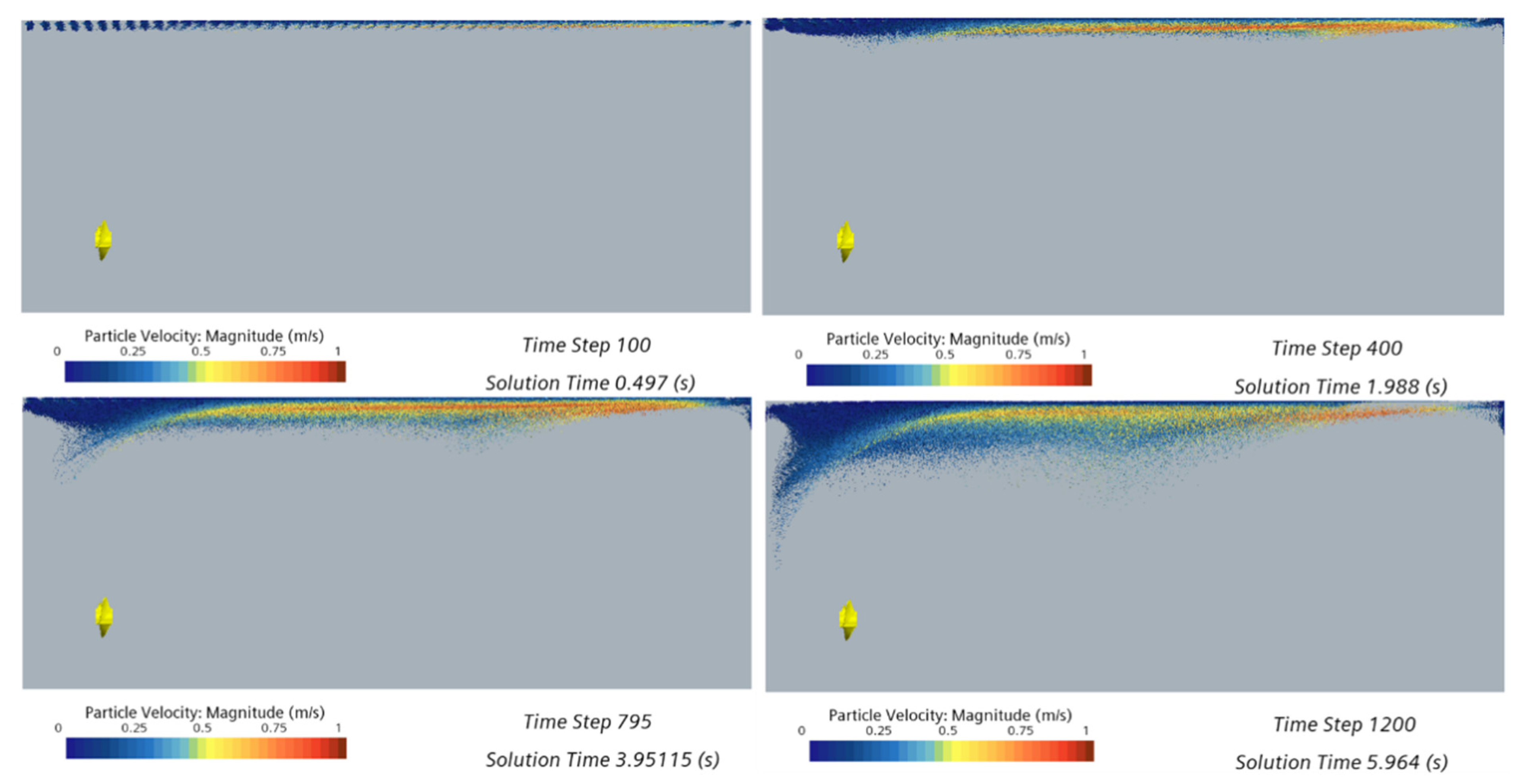
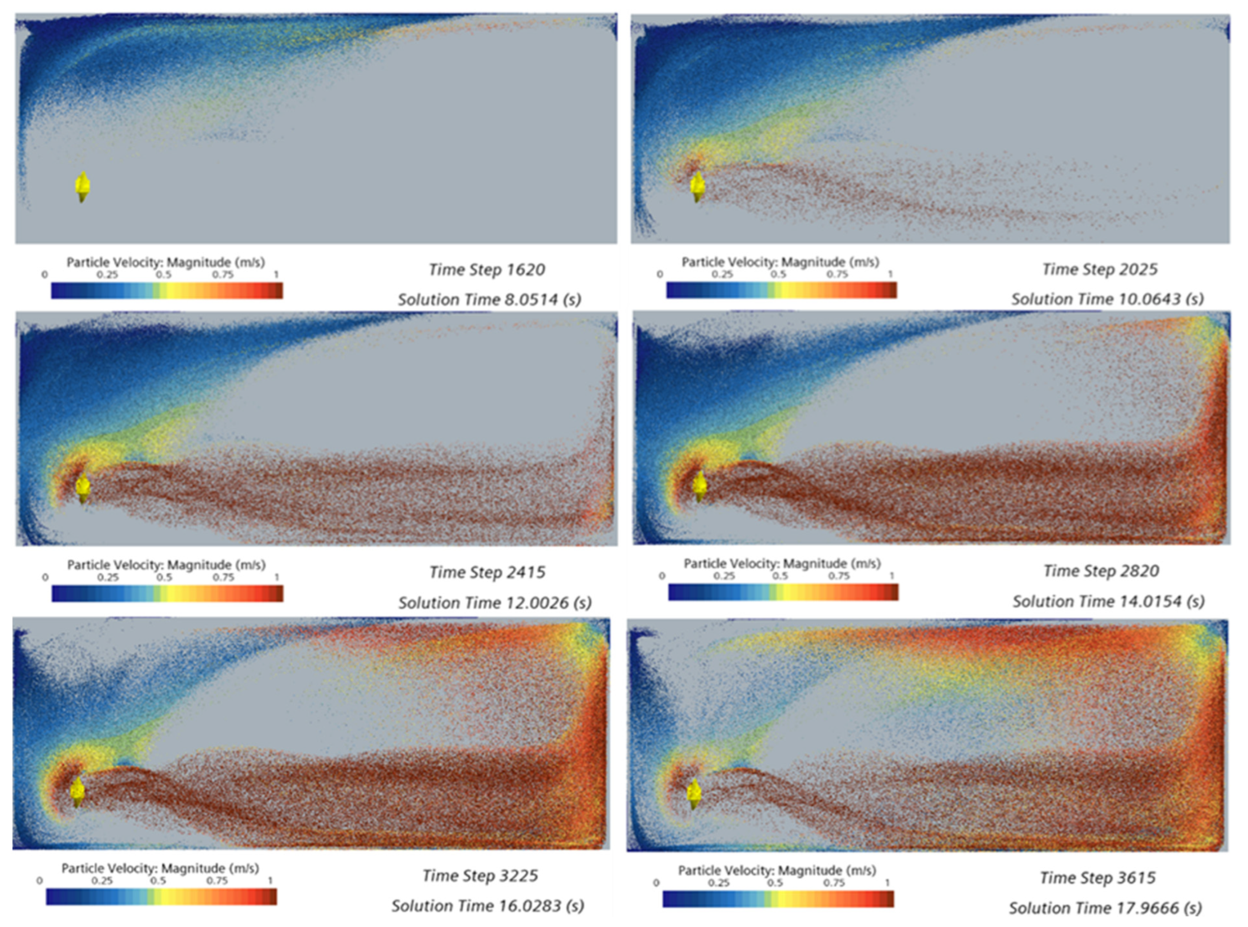
4.2.1. Motion Process of Particles

The movement of particles inside the pool is divided into approximately three stages: horizontal development stage, absorption-injection stage, and reflux-mixing stage. Particles begin to enter at 0 s and reach a stable number at 4 s. Due to the small density of particles and the weak velocity and turbulence intensity of the flow field near the water surface, as well as the influence of the pressure gradient force in the vertical direction, particles mainly accumulate in large quantities near the water surface during this time period. The particles downstream move in the horizontal direction under the drag force of the continuous phase of reflux and gather in the upstream of the pool; this stage is called horizontal development stage, as shown in Figure 9. At this time, the overall velocity of particles is low, and some high-speed particles exist in the middle and downstream regions.

At approximately 8 s, particles gather in large quantities in the region above the submersible mixer. The suction of the submersible mixer blades to the flow field and the reflux drive particles together to the suction surface of the submersible mixer. The inhaled particles gain a large amount of energy and velocity and are subsequently ejected from the working surface in a jet state, with particles reaching a maximum velocity of 10.1 m/s. This stage is called the absorption-injection stage, as shown in Figure 10.

After 20 s, almost all particles are ejected from the impeller and reach the downstream of the pool at a higher speed. A large number of particles near the wall will flow back in all directions under the action of continuous phase reflux, making the mixing of particles in the flow field gradually uniform. Part of the refluxed particles will enter the impeller of the submersible mixer again and move in the form of a jet. A part of the refluxed particles will make a secondary reflux after reaching the upstream wall. The particles of the secondary reflux have a large kinetic energy. The inertial force makes some particles overcome the suction effect of the submersible mixer blades no longer into the mixer but along the wall of the pool for movement. The secondary refluxed flow can drive particles deposited beneath the submersible mixer and prevent them from being deposited at the bottom of the pool, eventually forming two vortices near the wall. This stage is called the reflux-mixing stage; it is an essential stage to achieve uniform mixing in the submersible mixing flow field, as shown in Figure 11.

According to Formula (20), the velocity uniformity of particles is defined as follows:

$${\mathsf{\Upsilon }}_{pv}=1-\frac{{\displaystyle {\displaystyle \sum }_p}\left|v_p-\overline{v}\right|}{2\overline{v}{n}_p}$$

(21)

where $v_p$ is the velocity of each particle, $\overline{v}$ is the average velocity of all particles, and $n_p$ is the number of particles.

The average value of particle velocity in this paper is 0.47 m/s, and the velocity uniformity of particles is 0.715. It is similar to the velocity homogeneity of the flow field.

Figure 12 shows the distribution area of particles with a velocity less than 0.05 m/s. Comparing with the dead zone location of the flow field, it can be seen that the location of the low velocity particles is approximately the same as the dead zone distribution of the flow field.

4.2.2. Axial Distribution of Particles

In order to study the distribution law of particles along the axial direction, the pool is divided into 10 regions uniformly in the axial direction, and the regions are named a1~a10, as shown in Figure 13.

Figure 14 shows the distribution and velocity of particles in each region. It can be seen from the diagram that the particle distribution position and velocity are approximately symmetrical, forming a high-speed particle area around the impeller axis. With the development of jet, particles gradually move radially away from centrifugal force under the action of inertial force. A certain quantity of particles accumulate in the region downstream of the pool near the wall (a10). As Figure 15 shows the thermal map of particle distribution in this region, due to the low velocity of the flow field and turbulent kinetic energy, a suspended accumulation of particles is formed at the junction of the pool wall and the water surface.

Statistics of the number of particles in different axial regions are shown in Figure 16. It can be found that the distribution of particles along the axial direction is relatively uniform, without a large number of aggregates in a certain region. According to Equation (20), the uniformity of particle distribution is defined as follows:

$${\mathsf{\Upsilon }}_p=1-\frac{{\displaystyle {\displaystyle \sum }_c}\left|n_c-\overline{n}\right|}{2\left|\overline{n}\right|C}$$

(22)

where $n_c$ is the number of particles in the region, $\overline{n}$ is the average number of all regions, and $C$ is the number of equalized regions.

The uniformity of the axial distribution of particles is calculated to be 0.91.

4.2.3. Horizontal Distribution of Particles

Divide the pool evenly into 10 regions along the direction parallel to the water surface, as shown in Figure 17. Name these areas as b1~b10.

As Figure 18 shows the number of particles in each region, combined with the distribution and velocity of particles in each region as Figure 19, it can be found that the number of particles in regions b1~b9 is relatively evenly distributed. Aggregation zones of particles appear in the center and downstream of the water surface in area b1. The number of particles in area b10 increases significantly and two vortices are formed at the bottom of the pool. In order to further analyze the distribution of particles at the bottom of the pool, a region of 5 mm from the bottom of the pool is taken for analysis, as shown in Figure 20. Figure 21 shows the thermal map of particle distribution in this region. Combined with the jet characteristics of the submersible mixer, it can be found that due to the scouring effect of the high-speed jet, there are very few particles in dotted line area in Figure 20. The scoured particles eventually form vortices on both sides of the high-speed jet area and gather in large quantities. This is because the scouring of the bottom of the pool by submersible mixer jets can reduce only the number of particles in the scoured area, and the velocity of the scouring has no vertical upward component, resulting in more serious aggregation of particles in other areas of the bottom of the pool. Therefore, the installation position of submersible mixer from the pool bottom should be further studied. In addition, the direction of the axial rotation of the jet leads to a significantly higher number of particles in the upper vortex position than in the lower vortex.

The uniformity of the horizontal distribution of particles is calculated to be 0.81.

4.2.4. Lateral Distribution of Particles

Divide the pool evenly into 10 regions along the lateral direction, as shown in Figure 22. Observe the number of particles inside each region and its distribution.

It can be seen from the axial distribution of particles that the particles on the left and right sides of the impeller axis plane as the symmetry plane have similar distribution laws. Therefore, we mainly observe the particle distribution in the region of c1~c5, as shown in Figure 23.

From the central region (c5), it can be found that particles move along the jet direction of the flow field and form a larger vortex in the downstream region near the wall with the first return of the flow field, as shown by the dotted line in Figure 23. The cross-sectional size of this vortex gradually decreases as the region approaches the wall, and the number of particles in the core region of the vortex is nearly zero.

As shown in Figure 24, the region near the left and right walls (c1, c10) has the maximum number of particles. The upstream position of these two regions, both form a vortex of a larger scale, as shown in Figure 25. The vortexes rotate in the same direction and are roughly symmetrical in position. The velocity is lower in the core region of the vortex, and the kinetic energy of the particles is lower. The particles gather near this region, which is a dense gathering region of particles in the whole pool. This phenomenon is caused by secondary reflux of particles. This phenomenon can drive the particle movement in the lower part of the submersible mixer and avoid the sedimentation and accumulation of particles in this position. Although the velocity of the particles in the vortex region is low, they still have a certain angular velocity, as shown in Figure 26.

The number of particles within each region is counted, as shown in Figure 25. It can be found that the number of particles near the wall (c1, c10) is higher, the number of particles in the left wall region (c1) is significantly more than the rest of regions. According to the statistics of the number of particles in these ten regions, the uniformity of lateral distribution of particles is calculated as 0.86.

Table 2. Summary and comparison of distribution uniformity.

Uniformity	Axial	Horizontal	Lateral	Pool
${\mathsf{\Upsilon }}_p$	0.91	0.81	0.86	0.86

shows the distribution uniformity of particles in three directions. It can be seen that the distribution uniformity of particles in the axial direction is the best; the distribution uniformity of particles in the horizontal direction is the worst. Comprehensive analysis can find that vortices are significant factors causing the non-uniform distribution of particles. The uniformity of particle distribution of the whole pool is 0.86, and the distribution of particles is relatively uniform.

4.2.5. Collision of Particles

The collision of particles inside the pool is mainly divided into particle–particle collisions and particle-wall collisions. Figure 27 shows the location of particle–particle collisions and particle–wall collisions inside the pool at 36 s.

The number of collisions between particles and walls at this moment is 22,926, and the number of collisions between particles and particles is 27,737. The aggregation of particles inside the pool mainly occurs in the vicinity of the vortex and walls inside the pool, and the areas with the highest number of particles in both horizontal and lateral directions are the b10 region and the c1 region. Comparing the distribution of particles in these two regions with the location of particle collisions, as shown in Figure 28 and Figure 29. The number of particle collisions in these two regions is 42,535, accounting for 84% of the total number of particle collisions. It indicates that the collision of particles mainly occurs in the aggregation zones of particles.

5. Conclusions

In this paper, the solid–liquid two-phase flow field of the submersible mixer is studied for the first time by using the coupled CFD-DEM method, and the motion characteristics and distribution law of particles inside the pool were analyzed from the scale of particles. In addition, the evaluation method of particle position and velocity distribution uniformity inside the pool is also proposed, which can better guide the engineering application. The following conclusions can be derived:

(1)

The movement process of activated sludge particles in the tank can be roughly divided into three stages: horizontal development stage, absorption-injection stage, and reflux-mixing stage;

(2)

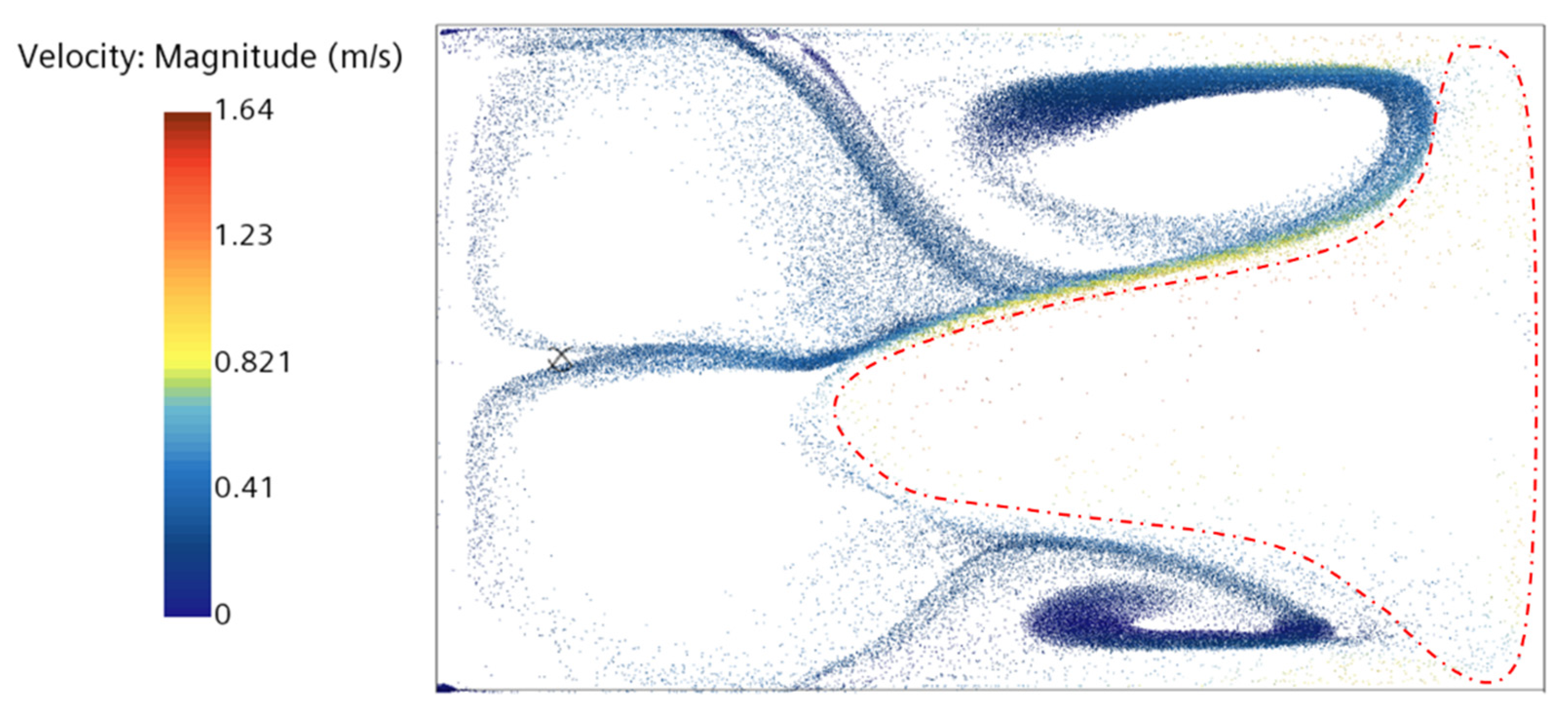
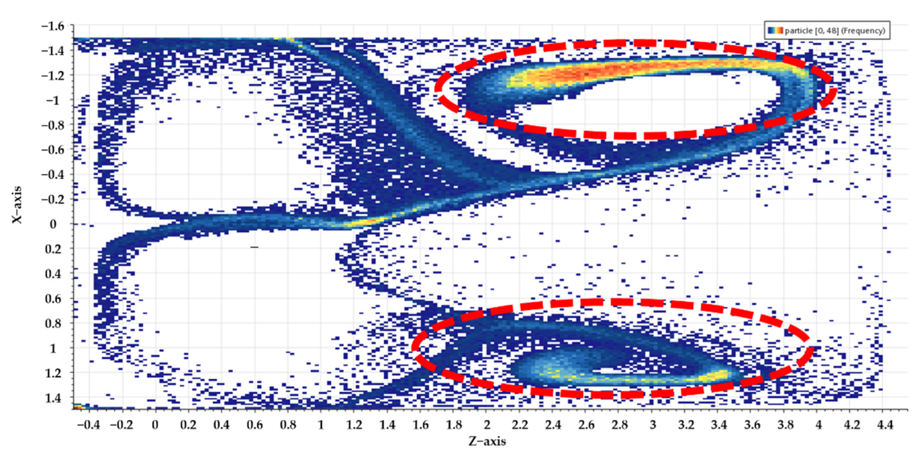
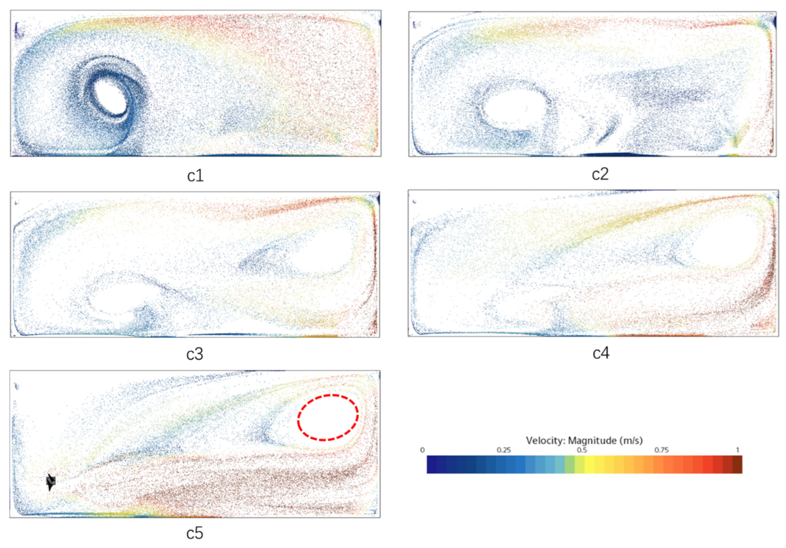
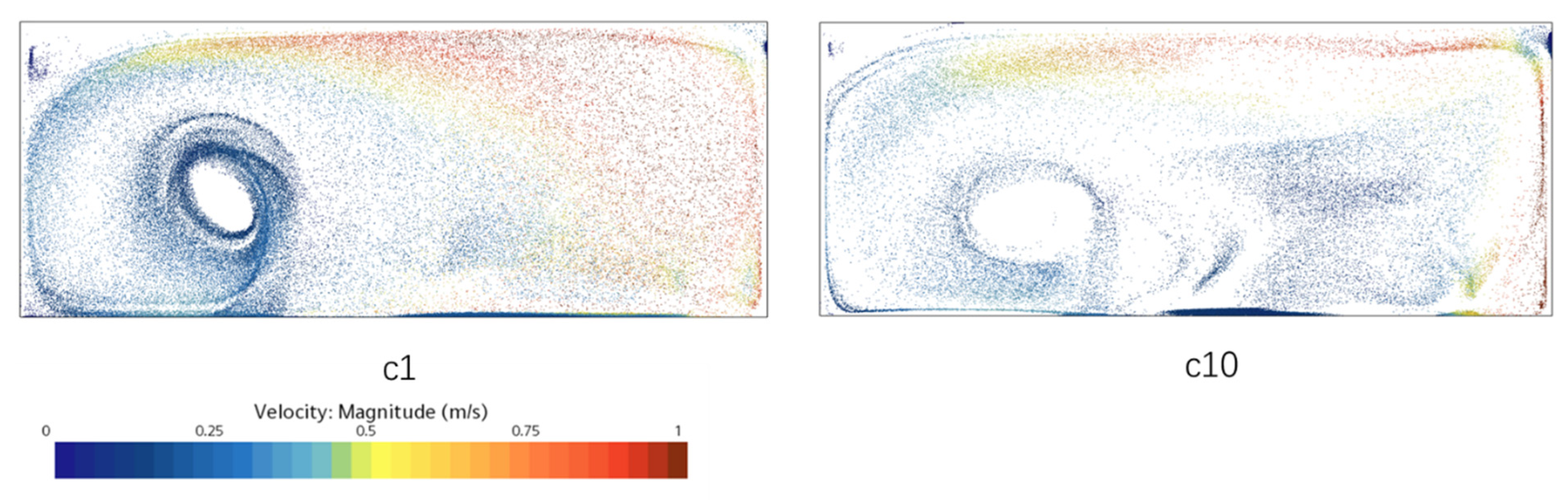
Particle accumulation occurs mainly in the dead zone of the flow field. There are two forms of particle aggregation: one is in the form of vortex, particles still have certain angular velocity; the other aggregation mainly occurs in the dead zone position of the pool wall junction, where the velocity and angular velocity of particles are relatively low;

(3)

The uniformity of particle distribution of the whole pool is relatively well, with the highest uniformity of distribution in the axial direction and the worst uniformity in the horizontal direction. The vortex generated near the bottom and walls of the pool is an essential factor leading to the aggregation of particles;

(4)

The collision of particles in the pool takes place mainly in the regions of particle aggregation, accounting for approximately 84% of the total number of particle collisions.

(5)

The coupled CFD-DEM-based method can simulate and study the solid–liquid two-phase flow of submersible mixers very well, and it can comprehensively analyze the motion and distribution of particles inside the pool. Based on this method, the optimization design of the solid–liquid two-phase flow field of the submersible mixer can be carried out more reasonably to achieve the effect of improving efficiency and saving energy.

References

1. Mackenziel, L.D.; David, A.C. Introduction to Environmental Engineering, 4th ed.; Tsinghua University Press: Beijing, China, 2007. [Google Scholar]
2. Yan, J.H.; Huang, D.J.; Teng, G.R. Research on Rural Domestic Sewage Disposal of Biologic Disposal High Efficiency Blender. J. Anhui Agric. Sci. 2009, 37, 9606–9607. [Google Scholar]
3. Xu, W.X.; Yuan, S.Q. Optimization Design of Submersible Mixer Based on a Simulation Study of Agitated and Engineering Application. China Rural. Water Hydropower 2011, 6, 32–35. [Google Scholar]
4. Xu, S.; Tang, F.P.; Wang, W.S. Influence of Different Blade Gaps on Flow Field of Submersible Mixer. China Water Wastewater 2017, 33, 106–109. [Google Scholar]
5. Ren, X.X.; Tang, F.P.; Xu, Y. Performance analysis of blade angle of submersible agitator. South-North Water Transf. Water Sci. Technol. 2021, 19, 805–813. [Google Scholar]
6. Li, W.; Wang, L.; Shi, W.D.; Chang, H.; Wu, P. Numerical simulation and performance prediction of solid-liquid two-phase flow of alkaline pump based on full factor test. J. Drain. Irrig. Mach. Eng. 2021, 39, 865–870. [Google Scholar]
7. Jin, J.H.; Zhang, H.W. A Numerical Simulation of Submersible Mixer in Three-dimensional Flow with Sewage-sludge Two-phase. China Rural. Water Hydropower 2014, 10, 159–162. [Google Scholar]
8. Tian, F.; Shi, W.; Jiang, H.; Zhang, Q. A Study on Two-Phase Flow of Multiple Submersible Mixers Based on Rigid-Lid Assumption. Adv. Mech. Eng. 2014, 2014, 531234. [Google Scholar] [CrossRef]
9. Cundall, P.A.; Strack, O.D.L. A Discrete Numerical Mode for Granular Assemblies. Géotechnique 1979, 29, 47–65. [Google Scholar] [CrossRef]
10. Li, Y.L. Effect of Continuously Varying Curvature on Solid-Liquid Two-Phase Flow by CFD-DEM and its Application in Large Desulfurization Pump; Jiangsu University: Zhenjiang, China, 2015. [Google Scholar]
11. Zhou, M.; Wang, S.; Kuang, S. CFD-DEM modelling of hydraulic conveying of solid particles in a vertical pipe. Powder Technol. 2019, 354, 893–905. [Google Scholar] [CrossRef]
12. Xia, C.; Zhao, R.J.; Shi, W.D. Numerical Investigation of Particle Induced Erosion in a Mixed Pump by CFD-DEM Coupled Method. J. Eng. Thermophys. 2021, 42, 357–369. [Google Scholar]
13. Zhao, L.J. Numerical Simulation for Stirred Mixing Based on CFD-DEM and Development of Integrated Simulation Platform; Zhejiang University of Technology: Hangzhou, China, 2021. [Google Scholar]
14. Song, L.B.; Teng, S.; Cao, Q.; Kang, C.; Ding, K.J.; Li, C.J. Wear of large solid particles on the impeller of solid-liquid two-phase flow pump. J. Drain. Irrig. Mach. Eng. 2021, 39, 987–993. [Google Scholar]
15. Schiller, V.L. Uber die Grundlegenden Berechnungen bei der Schwerkraftaufbereitung. Z. Vernes Dtsch. Inge 1933, 77, 318–321. [Google Scholar]
16. Dinh, B. Experiments on the lift of a spinning sphere in a range of intermediate Reynolds numbers. Exp. Fluids 1998, 25, 16–22. [Google Scholar]
17. Saffman, P.G. The Lift on a Small Sphere in a Slow Shear. J. Fluid Mech. 1965, 22, 385–400. [Google Scholar] [CrossRef] [Green Version]
18. Chen, Y.F.; Yang, C.; Zhang, H. Influence and optimization of mixer’s arrangement of flow field of anoxic pool. J. Drain. Irrig. Mach. Eng. 2020, 38, 1045–1050. [Google Scholar]
19. Xu, D.E.; Yang, C.X.; Cai, J.G.; Han, Y.; Ge, X.F. Numerical simulation of solid-liquid two-phase in tubular turbine. J. Drain. Irrig. Mach. Eng. 2021, 39, 910–916. [Google Scholar]
20. Zhang, X.N.; Zhao, J.Y.; Wang, W.H. Influence of Submersible Mixer Installation Angle with the Mixing Effect. J. Beijing Inst. Civ. Eng. Archit. 2014, 30, 48–51. [Google Scholar]
21. Weltens, H.; Bressler, H.; Terres, F. Optimisation of Catalytic Converter Gas Flow Distribution by CFD Prediction. In Proceedings of the International Congress & Exposition, Detroit, MI, USA, 1–5 March 1993. [Google Scholar]
Figure 1. Arrangement of submersible mixer.
Energies 15 06096 g001
Figure 2. Meshing of impeller and pool.
Energies 15 06096 g002
Figure 3. The velocity and turbulent kinetic energy bubble plots of four axial planes along Z-axis direction: (a) Y = 0 plane; (b) Y = −0.3 plane; (c) Y = −1 plane; (d) Y = −1.3 plane.
Energies 15 06096 g003
Figure 4. Velocity streamline diagram of full flow field.
Energies 15 06096 g004
Figure 5. Velocity contour of multiple axial sections.
Energies 15 06096 g005
Figure 6. The distribution of the dead zone.
Energies 15 06096 g006
Figure 7. The velocity contour and vector diagram of Y = 0 plane.
Energies 15 06096 g007
Figure 8. Particle trajectory diagram.
Energies 15 06096 g008
Figure 9. Horizontal development stage.
Energies 15 06096 g009
Figure 10. Absorption-injection stage.
Energies 15 06096 g010
Figure 11. Reflux-mixing stage.
Energies 15 06096 g011
Figure 12. Distribution area of low velocity particles.
Energies 15 06096 g012
Figure 13. Regions of the flow field divided along the axial direction.
Energies 15 06096 g013
Figure 14. Location and velocity distribution of particles in a1~a10.
Energies 15 06096 g014
Figure 15. Thermal map of particles distribution in a10.
Energies 15 06096 g015
Figure 16. Number of particles in a1~a10.
Energies 15 06096 g016
Figure 17. Regions of flow field divided along horizontal direction.
Energies 15 06096 g017
Figure 18. Number of particles in b1~b10.
Energies 15 06096 g018
Figure 19. Location and velocity distribution of particles in b1~b10.
Energies 15 06096 g019
Figure 20. Location and velocity distribution of particles in the region of 5 mm from the bottom of pool.
Energies 15 06096 g020
Figure 21. Thermal map of particles distribution in the region of 5 mm from the bottom of pool.
Energies 15 06096 g021
Figure 22. Regions of flow field divided along the lateral direction.
Energies 15 06096 g022
Figure 23. Location and velocity distribution of particles in c1~c5.
Energies 15 06096 g023
Figure 24. Number of particles in c1~c10.
Energies 15 06096 g024
Figure 25. Location and velocity distribution of particles in c1 and c10.
Energies 15 06096 g025
Figure 26. Location and angular velocity distribution of particles in c1.
Energies 15 06096 g026
Figure 27. Collision of particles: (a) Particle–particle collisions; (b) Particle–wall collisions.
Energies 15 06096 g027
Figure 28. Location and collision of particles in b10: (a) Location of particles; (b) Collision of particles.
Energies 15 06096 g028
Figure 29. Location and collision of particles in c1: (a) Location of particles; (b) Collision of particles.
Energies 15 06096 g029