Probabilistic Peak Demand Estimation Using Members of the Clayton Generalized Gamma Copula Family

Abstract

Climate change impacts many aspects of life and requires innovative thinking on various issues. The electricity sector is affected in several ways, including changes in the production components and consumption patterns. One of the most important issues for Independent System Operators, a state-controlled organization responsible for ensuring the reliability, availability, and quality of electricity delivery in the country, is the response to climate change. This is reflected in the appropriate design of production units to cope with the increase in demand due to extreme heat and cold events and the development of models aimed at predicting the probability of such events. In our work, we address this challenge by proposing a novel probability model for peak demand as a function of wet temperature (henceforth simply temperature), which is a weighting of temperature and humidity. We study the relationship between peak demand and temperature using a new Archimedean copula family, shown to be effective for this purpose. This family, the Clayton generalized Gamma, is a multi-parameter copula function that comprises several members. Two new measures of fit, an economic measure and a conditional coverage measure, were introduced to select the most appropriate family member based on the empirical data of daily peak demand and minimum temperature in the winter. The Clayton Gamma copula showed the lowest cost measure and the best conditional coverage and was, therefore, proven to be the most appropriate member of the family.

1. Introduction

Climate change leads to extreme temperatures that last for extended periods. These have a significant impact on electricity demand, mainly due to the use of cooling and heating systems [1,2]. The increase in electricity demand requires a systematic assessment of both infrastructure and long-term planning. For the short term, proper evaluation of electricity demand allows the system operator to take corrective actions. These include delaying the shutdown of generating units for maintenance and preparing immediate generating units to respond to a decrease in remaining reserve power. In the long term, properly assessing electricity demand can help design the system to meet potential increases and address peak demands [3]. Peak demand is a critical and challenging issue since it may exceed production capacity and results in load shedding and service disruption for consumers [4,5]. It also impacts electric utilities as production units are subject to higher extreme temperatures, precipitation, and wind strength changes, which could lead to power outages [6]. In Israel, global warming affects the length of the seasons. The summers are getting longer and warmer and the transitional seasons are getting shorter. Last year (2022), the winter was relatively extremely cold. In 2020, during one week in May (transitional season) and in September 2021 (summer season), unpredictable extreme hot temperatures were observed. In January 2022 (winter season) and March (transitional season), the lowest temperature was recorded for the last hundred years. In view of these changes, peak demand estimation requires a better understanding of the relationship between electricity demand and temperature. The study of this relationship has a long history, and a variety of methods have been described in the literature. Reference [7] reviewed the models since 1918, mostly using regression techniques. By [8], many methods have been used for short-term load forecasting, including multiple regression, exponential smoothing, and state-space methods. Reference [9] stated that data availability and technological development made it possible to develop new statistical models, such as hierarchical load forecasting (HLF), for forecasting small areas’ electricity demand. Reference [10] used an autoregressive distributed lag model with socio-economic data to examine the impact of climate change on electricity. A regression time series model introduced by [11] estimated the response function of average and peak loads to weather, using daily average temperature and total daily precipitation. Reference [12] reviewed fifty different forecasting methods from 483 energy planning models and showed that forty percent of the energy models use neural networks, in addition to support vector machine, ARIMA, and linear regression models, which are also widely used. Reference [13] developed models for estimating demand by extending a linear regression model to a probabilistic Bayesian framework and demonstrated improvements in mean absolute error in real case studies. Using MAPE, Reference [14] showed that multiple linear regression seasonality models outperformed machine learning methods in predicting daily peak loads in South Korea. A multivariate hybrid prediction model using a neural network and a pre-processing algorithm incorporating reactive consumption, humidity, and temperature was used by [15] to predict the hourly electricity consumption of a hospital.

In recent years, two further research directions of estimating electricity demand, emphasizing peak demand, have gained interest. These entail reliance on a probabilistic forecasting approach and the use of copula functions.

Probabilistic load forecasting has become very important to energy system planning and operation. This approach addresses the pitfall in the classical forecasting approach, which evaluates the demand for electricity in a deterministic way, i.e., a single expected value for the predicted load is provided without considering the inherent error in the model. This can be addressed by calculating an ensemble of multiple points for a future load probability. Some of the approaches that assimilate the weather uncertainty were discussed in [9,16,17,18,19].

Copula functions characterize the relations between the variables with complex nonlinear dependence structures. This is achieved through separate modeling of the marginal distributions of the underlying variables and their dependence structure. Reference [20] developed a probabilistic model to estimate peak demand for smart cities using smart meters and socio-demographic data. To model the nonlinear dependence structure between different consumers, a variable truncated R-vine copula (VTRC) was used. A short-term deep learning prediction model for peak demand was introduced by [21]. They used a Box–Cox transformation for the load data adaptation and a copula function to characterize the relation between peak demand and temperature. Reference [22] modeled the relationship between minimum daily electricity demand and maximum daily temperature and used a multi-parameter compound Archimedean copula with a flexible dependence structure, which increased the flexibility of the dependence structure and improved the fit to the data. Reference [23] evaluated peak electricity demand using Gaussian mixture models and copula functions and provided a time-correlated statistical model. For additional references on the application of copula functions, see [24,25,26,27,28].

Our study addresses the significant issue of estimating peak demand with a probability approach using a copula function. We use a novel Archimedean copula family, the Clayton generalized Gamma, first reported in [29], to characterize the dependence structure between the minimum temperature and daily peak demand in the winter. This three-parameter family includes several members and permits enhanced flexibility when determining which copula function to use based on empirical data. In Section 2, we give a brief introduction to copula functions, the compound Archimedean copula, and the Clayton generalized Gamma (CGG) family. In Section 3, we derive the value-at-risk and the confidence interval of peak demand using the CGG family. Section 4 introduces the statistical process for parameter estimation and peak demand confidence interval evaluation. The description of the data structure, the experiment, and the results of a numerical study are presented in Section 5. Conclusions are given in Section 6.

2. Copula Function

Characterizing the interaction between variables is an essential tool for modeling many phenomena, and various methods have been suggested to address this issue. Usually, two random variables are described by a bivariate distribution, where both random variables have the same parametric univariate distribution. Using copula functions eliminates this restriction by separating the dependence structure of the variables from their marginal distribution [30]. By [31], every multivariate cumulative distribution function $F\left(x_1,\dots ,x_d\right)=P\left(X_1\le x_1,\dots ,X_d\le x_d\right)$ of a random vector $\left(X_1,\dots ,X_d\right)$ can be uniquely written in terms of the separate parts of its marginals $F_i\left(x_i\right)=P\left(X_i\le x_i\right)$, which are a set of cumulative univariate distributions, and copula $C,$ which holds the dependence structure between the variables, such as

$$F\left(\mathbf{x}\right)=P\left(X_1\le x_1,...,X_d\le x_d\right)=C\left(F_1\left(x_1\right),\dots ,F_d\left(x_d\right)\right),$$

(1)

for $x_i\in \left(-\infty ,\infty \right),i=1,\dots ,d.$ This function was extensively reported in [32,33,34]. Among the best-known family of copulas is the Archimedean family, characterized by its generator function; hence, different choices of generator functions lead to different copulas with their respective expression of dependence. A two-dimensional Archimedean copula is denoted by:

$$C_{\theta }\left(u,v\right)={\phi }_{\theta }^{-1}\left({\phi }_{\theta }\left(u\right)+{\phi }_{\theta }\left(v\right)\right),$$

(2)

where ${\phi }_{\theta }\left(t\right)$ is the Archimedean generator and $\theta$ is the dependence parameter. The generator $\phi$ is a continuous, strictly decreasing convex function $\phi :\left[0,1\right]\to \left[0,+\infty \right]$ such that ${\phi }_{\theta }\left(1\right)=0$.

2.1. Inverse Compound Archimedean Copula

The Archimedean family contains a wealth of parametric functions with a variety of dependence structures. However, most of them consist of a single dependence parameter, limiting the flexibility of fitting the data. New novel methods to expand the number of Archimedean dependence parameters were introduced in [29]. This was based on the creation of novel inverse Archimedean generators by compounding an existing inverse generator ${\phi }_{\theta \left(v\right)}^{-1}\left(t\right)$ with respect to $\tilde{g}\left(v\right)$, a probability density of parameter $v=v\left(\theta \right),$ which is a one-to-one function of the dependence parameter $\theta$. We denote the compound inverse generator as $h\left(t\right)$ such that

$$h\left(t\right)={\int }_V{\phi }_{\theta \left(v\right)}^{-1}\left(t\right)\tilde{g}\left(v\right)dv.$$

(3)

A different approach reported in [35] used a compound of an existing generator ${\phi }_{\theta \left(v\right)}\left(t\right)$ with respect to $\tilde{g}\left(v\right)$, such as

$$h\left(t\right)={\int }_V{\phi }_{\theta \left(v\right)}\left(t\right)\tilde{g}\left(v\right)dv.$$

(4)

2.2. Clayton Generalized Gamma Family

The CGG family is generated by compounding the inverse generator of the Clayton copula, when the generalized Gamma is the density function of parameter $v=v\left(\theta \right)$:

$$\tilde{g}\left(v\right)=\left[\left(\frac{p}{{\alpha }^d}\right)v^{d-1}{e}^{-{(v/\alpha )}^p}\right]\frac{1}{\mathsf{\Gamma }\left(d/p\right)},$$

(5)

where $v\in \left(0,\infty \right)$ and $p,\alpha ,d>0$. The Clayton copula is the most commonly used Archimedean copula in many areas, defined as

$$C_{\theta }(u,v)={\left(u^{-\theta }+v^{-\theta }-1\right)}^{-\frac{1}{\theta }},$$

(6)

for $\theta \ge 0$. The generator function is given by

$${\phi }_{\theta }\left(t\right)=\left(t^{-\theta }-1\right)$$

(7)

and the inverse generator function is

$${\phi }_{\theta }^{-1}\left(t\right)={\left(t+1\right)}^{-1/\theta }.$$

(8)

We chose the generalized Gamma as a compounding distribution since it is a rich family comprising some well-known distributions, described in

Table 1. Members of the generalized Gamma distribution [36].

Family	p	$\mathit{\alpha }$	d
Gamma	1	a	d
Standard Gamma	1	1	d
Wein	1	a	4
Nakagami	2	a	d
Half Normal	2	a	1
Folded Normal	2	$\sqrt{2}$	1
Rayleigh	2	a	2
Maxwell–Boltzmann	2	a	3
Wilson–Hilferty	3	a	$d/3$
Weibull	p	a	$d=p$

.

By using Equation (3), a new generator of the Clayton generalized Gamma family is derived:

$$\begin{array}{ccc}\hfill h\left(t\right)& =& \frac{1}{\mathsf{\Gamma }\left(d/p\right)}{\int }_V\left(\frac{p}{{\alpha }^d}\right)exp\left(-v^{p}ln\left(t+1\right)\right)\left[v^{d-1}{e}^{-{(v/\alpha )}^p}\right]dv\hfill \\ & =& {\left((1+\alpha {\left(ln\left(t+1\right)\right)}^{\frac{1}{p}})\right)}^{-d}.\hfill \end{array}$$

(9)

Using Equation (2), a new bivariate compound copula, the CGG, is now obtained:

$$C(u,v)={\left(1+\alpha {\left(ln\left(exp\left({\left((\frac{1}{u^{1/d}}-1)/\alpha \right)}^p\right)+exp\left({\left((\frac{1}{v^{1/d}}-1)/\alpha \right)}^p\right)-1\right)\right)}^{\frac{1}{p}}\right)}^{-d},$$

(10)

for $p>0,\alpha >0,d>0.$ This three-parameter copula family expands the one-parameter Clayton copula and comprises 10 notable members, each corresponding to a particular case of the generalized Gamma distribution and dictated by the choice of $\alpha ,d$, and p, as described in Table 1.

3. Value-at-Risk of Electricity Demand

We aim to assess electricity demand for any given temperature. To this end, we need to evaluate the confidence interval that expresses the forecast error of peak demand. This can be derived from the demand’s conditional value-at-risk (VaR), an approach to quantifying the risk of extreme events, given the temperature, i.e., $Va{R}_q\left(X\right)=min\left(t|F_X\left(t\right)\ge q\right)$ is the lower q-percentile of the random variable X with cumulative distribution function $F_X\left(t\right)=P\left(X\le t\right).$ Utilizing $VaR$ enables the calculation of the confidence interval, which provides a probabilistic estimate of peak demand. To establish the $VaR$, we need the following proposition:

Proposition 1.

Let X and Y be two random variables with cumulative distribution functions $F_X\left(x\right)$ and $F_Y\left(y\right)$. Suppose the dependence structure of the bivariate vector $(X,Y)$ is defined with copula $C(u,v)$, where $u=F_X\left(x\right)$ and $v=F_Y\left(y\right)$. Let $C_2(u,v)=\frac{\partial }{\partial v}C(u,v)$ be the first derivative of the copula function with respect to v and $C_{1,2}(u,v)=\frac{{\partial }^2}{\partial u\partial v}C(u,v)$ be the derivative of $C_2(u,v)$ with respect to u. Then, the q-level value-at-risk of the first variable X given $Y=y,Va{R}_q\left(X\right|Y=y)$ is defined by the solution of the following equation with respect to t:

$$C_2(F_X\left(t\right),F_Y\left(y\right))=q,q\in (0,1).$$

(11)

Proof. 

Clearly, we need to establish that $F_{X|Y}\left(t\right|Y=y)=C_2(F_X\left(t\right),F_Y\left(y\right))$. The joint density function of X and Y is given by

$$f_{X,Y}(x,y)=C_{1,2}(F_X\left(x\right),F_Y\left(y\right))f_X\left(x\right)f_Y\left(y\right).$$

Then

$$\begin{array}{ccc}\hfill F_{X|Y}\left(t\right|Y& =& y)={\int }_{-\infty }^t\frac{C_{1,2}(F_X\left(x\right),F_Y\left(y\right))f_X\left(x\right)f_Y\left(y\right)}{f_Y\left(y\right)}dx\hfill \\ & & ={\int }_{-\infty }^t{C}_{1,2}(F_X\left(x\right),F_Y\left(y\right))f_X\left(x\right)dx\hfill \\ & =& {\int }_{-\infty }^t{C}_{1,2}(F_X\left(x\right),F_Y\left(y\right))d{F}_X\left(x\right)\hfill \\ & =& {\int }_0^{F_X\left(t\right)}{C}_{1,2}(\xi ,F_Y\left(y\right))d\xi \hfill \\ & =& C_2(F_X\left(t\right),F_Y\left(y\right))\hfill \end{array}$$

□

To obtain a confidence interval for the demand given the temperature using the CGG family (10) and Proposition 1, we need to obtain the first derivative of the copula with respect to v. Let $K(u,v)$ be denoted by

$$K(u,v)=ln[exp({(\frac{(u^{-1/d}-1)}{\alpha })}^p)+exp({(\frac{(v^{-1/d}-1)}{\alpha })}^p)-1].$$

Then the first derivative of bivariate copula $C(u,v)$ with respect to v is

$$\begin{array}{c}{C}_2(u,v)=\frac{d}{dv}{\left(\left[1+a{\left(K(u,v)\right)}^{\frac{1}{p}}\right]\right)}^{-d}\\ =\frac{\left[\begin{array}{c}\left(\left(v^{-1/d-1}exp{\left((v^{-1/d}-1)/a\right)}^p\right){\left((v^{-1/d}-1)/a\right)}^{p-1}\right)\\ \left(v^{-1/d-1}exp({(\frac{(v^{-1/d}-1)}{\alpha })}^p){(\frac{(v^{-1/d}-1)}{\alpha })}^{p-1}{\left(K(u,v)\right)}^{\frac{1}{p}-1}{\left(\left[1+a{\left(K(u,v)\right)}^{\frac{1}{p}}\right]\right)}^{-d-1}\right)\end{array}\right]}{\left(exp({(\frac{(u^{-1/d}-1)}{\alpha })}^p)+exp({(\frac{(v^{-1/d}-1)}{\alpha })}^p)-1\right)}.\end{array}$$

(12)

Equation (12) is used to calculate the confidence interval of the daily peak demand as described in the next section.

4. Statistical Process

In this section, we present the statistical method for calculating the confidence interval for peak electricity demand, using $Va{R}_q\left(X\right|Y)$. The method consists of four steps, as shown in Figure 1.

The following is a detailed description of each step.

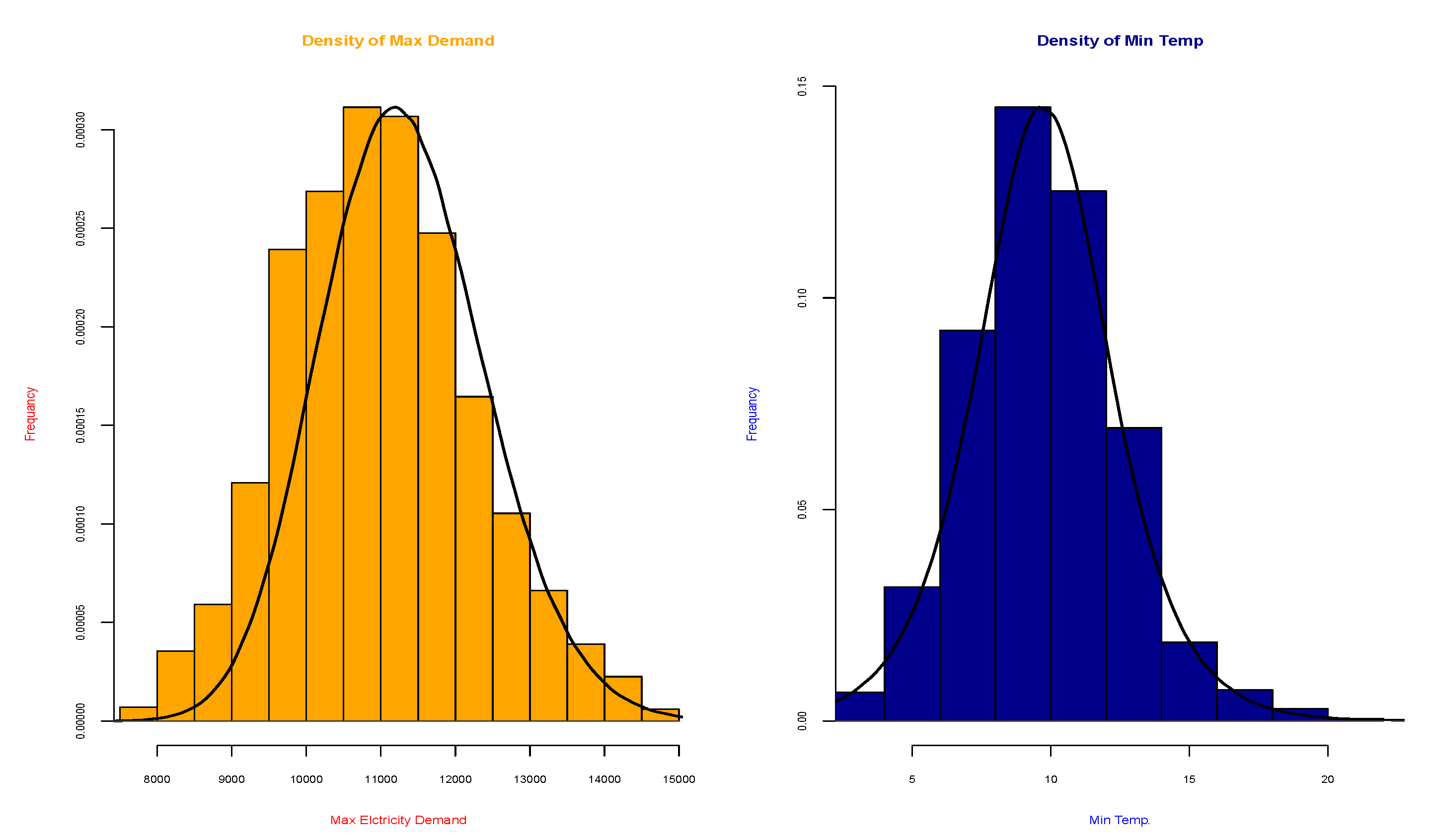
4.1. Identification of the Marginal Distributions

The first step in finding a copula is to determine the marginal distributions of the underlying variables, as defined in Equation (1). The EasyFit software was used to analyze the empirical data, to identify the desired best-fitting distributions, and to estimate their parameters. The distribution with the lowest Anderson–Darling test score was chosen for each of the variables.

4.2. Estimation of the Parameters for Members of the CGG Family

The conditional distribution shown in Equation (12) contains three parameters, i.e., $(p,a,d)$. Changing the parameter values results in a different member of the CGG family. For example, when $p=1$ and a and d are the estimated parameters, the first member in Table 1 is the Clayton Gamma copula, which results from compounding the Clayton copula with the Gamma distribution. In order to estimate k parameters, one would need to consider k dependence measures. In our work, we needed two dependence measures at most for estimating the parameters. The parameter values are those for which the theoretical dependence measure of the copula function is equal to their empirical values. A description of the estimating methodology can be found in [35].

In this work, since $k\le 2$, we used two copula-based measures of multivariate association, the Gini Gamma and the Blomqvist beta. These two measures are tools for quantifying the dependence of nonlinear association. Gini’s Gamma is a measure of association based on the concordance between a pair $(X,Y)$ with copula $C(u,v)$, the Fréchet upper bounds M, and the Fréchet lower bounds W [29,37,38]. Blomqvist’s beta is a measure that describes the relationship between a pair of observations regarding their quadrants [29,39]. The measures are given by the following.

Gini’s Gamma$\left(\mathsf{\Gamma }\right)$:

The Gini Gamma is defined by

$$\begin{array}{ccc}\hfill \mathsf{\Gamma }& =& 4\left[{\int }_0^{1}C\left(u,1-u\right)du-{\int }_0^1\left[u-C\left(u,u\right)\right]du\right].\hfill \end{array}$$

(13)

For a random sample $\left(X_1,Y_1\right),\dots ,\left(X_{n,}{Y}_n\right)$ with associated ranks $\left(R_1,S_1\right),\dots ,\left(R_{n,}{S}_n\right)$, the estimated measure is given by

$$\widehat{\mathsf{\Gamma }}=\frac{2}{n^2}\sum _{i=1}^n\left\{\left|(n+1-R_i)-S_i\right|-\left|R_i-S_i\right|\right\},$$

(14)

Blomqvist’s beta$\left({\beta }_l\right)$:

Blomqvist’s beta is defined by

$${\beta }_l=4C\left(\frac{1}{2},\frac{1}{2}\right)-1.$$

(15)

The estimated measure is given by

$${\widehat{\beta }}_l=\frac{2}{n}\sum _{i=1}^{n}I\left(\left(R_i-\frac{n+1}{2}\right)\left(S_i-\frac{n+1}{2}\right)\ge 0\right)-1.$$

(16)

To establish the parameters of each member of the CGG, one needs to equate Equation (13) to Equation (14) and/or Equation (15) to Equation (16), depending on the number of unknown parameters.

4.3. Calculation of Confidence Intervals of Electricity Peak Demand

Recall that X is the daily peak demand, Y is the daily minimum temperature, and $u=F_X\left(x\right)$ and $v=F_Y\left(y\right)$, then by placing u, v, and the estimated copula parameters, explained in Section 4.2, into Equation (12), $Va{R}_q\left(X\right|Y=y),$ characterized by the conditional copula function $C_2(u,v)$, can be established. For each temperature value, we can obtain the $(1-\alpha )$ confidence interval for the demand peak:

$$[Va{R}_{\frac{\alpha }{2}}\left(X\right|Y=y);Va{R}_{1-\frac{\alpha }{2}}\left(X\right|Y=y)].$$

(17)

This procedure is performed for each member of the CGG family in Table 1.

4.4. Finding the Best Copula Function

Given the large number of copula functions available, it is challenging to select the best one. Reference [40] used minimization of the distance between the parametric distribution function $k_{\theta }\left(v\right)=P\left(C(X,Y)\le v\right)$ and its empirical counterpart $k_n\left(v\right),$ i.e., minimizing $\int {\left[K_{\theta }\left(v\right)-K_n\left(v\right)\right]}^{2}d{K}_n\left(v\right),$ to determine the appropriated Archimedean copula function that fits the data best. Reference [41] used the QQ-plot of these functions. Reference [42] suggested that the best-fitting copula is the one closest to the empirical copula in the $L^2$-norm, i.e., $d_2\left(C_n,C_{\theta }\right)={∥C_{\theta }-C_n∥}_{L^2}.$ We attempted to identify the member of the CGG that fits the data best through two fitting measures: the conditional coverage measure denoted by $\left(CC\right)$ and the economic cost measure denoted by $\left(CM\right)$.

4.4.1. The Conditional Coverage Measure

This measure examines the percentage of the number of observations that are contained within the $(1-\alpha )$ confidence interval boundaries, as defined by the conditional $Va{R}_q\left(X\right|Y=y)$.

Let $Z_i$ be an indicator of $(i=1,\dots ,n)$, such as

$$Z_i=\left\{\begin{array}{cc}1\hfill & C_2{(u,v)}_{{\left[0.005\right]}_i}<M{D}_i<C_2{(u,v)}_{{\left[0.995\right]}_i}\hfill \\ 0\hfill & \mathrm{otherwise}\hfill \end{array}\right.,$$

where $M{D}_i$ is the max electricity demand in day i. Then, the average conditional coverage is

$$CC=\frac{{\sum }_{i=1}^n{Z}_i}{n},$$

(18)

where n is the number of observations. The most appropriate copula function is the one for which $CC$ is closest to $(1-\alpha )$.

4.4.2. Example

In this example, we illustrate the calculation of the conditional coverage. In Figure 2 below, we show one member of the CGG family, the Clayton–Wien copula. The red dots are the empirical daily peak demand, and the blue and gold lines are the $0.99\%$ confidence boundaries. All the observation below the blue line (the upper $0.995$ confidence limit) and above the gold line (the lower $0.005$ confidence limit) are the covered observations. Using Equation (18), the $CC$ measure can be obtained.

4.4.3. The Economic Cost Measure

The Independent System Operator organizations are responsible for ensuring the reliability and availability of electricity delivery. In particular, they are entrusted with the responsibility to ensure the economic well-being of their customers. Hence, choosing a model should be based on probabilistic and economic considerations. Much work has been invested in attempting to estimate the price of underestimating peak demand, i.e., the value of lost load (VOLL). This depends on several factors, including the type of customer, regional economic and demographic conditions, the timing and duration of power outages, and others [43]. For more details, see [44,45,46]. In our work, we assumed that the VOLL was set at USD 30 per KW and the cost of overestimation was set at USD $0.15$ per KW. The cost measure’s (CM) definition is presented as follows:

Let $M{D}_i$ be the maximum demand in day $\left[i\right]$ and $C{M}_i$ be a cost function that expresses the magnitude of the cost of error with respect to the upper bound $C_2{(u,v)}_{{\left[0.995\right]}_i}$:

$$C{M}_i=\left\{\begin{array}{cc}0.15\$\ast |M{D}_i-C_2{(u,v)}_{{\left[0.995\right]}_i}|\hfill & M{D}_i<C_2{(u,v)}_{{\left[0.995\right]}_i}\hfill \\ 30\$\ast |M{D}_i-C_2{(u,v)}_{{\left[0.955\right]}_i}|\hfill & M{D}_i>C_2{(u,v)}_{{\left[0.995\right]}_i}\hfill \end{array}\right..$$

(19)

A possible procedure is to calculate the average of $C{M}_i$ across all days $\left[i\right]$. This approach is inappropriate since it ignores the underestimation of peak demand, which is much more detrimental at low winter temperatures, the season this work focused on. This is because low temperatures lead to a significant increase in heating, which leads to high peak demand and requires special evaluations of the operation system. In order to address this, we offer a new weight cost measure, which is a multiplication of $C{M}_i$ with a weight index, which we call the power exponential linear weight (PeLw).

Let T be a continuous random variable with $t_i\in \left[0,22\right],$ a range representing the minimum temperature in the Israeli winter, i.e., $min\left(t_i\right)=0$ and $max\left(t_i\right)=22$. Then, the linear weight for each temperature is given by

$$L{W}_i=\frac{t_i-min\left(t_i\right)}{max\left(t_i\right)-min\left(t_i\right)}.$$

Using $L{W}_i$, the PeLw is defined by

$$PeL{w}_i=exp(k·L{W}_i)-1,$$

(20)

and the new weighted cost measure is

$$C{M}_w=\frac{{\sum }_i^{n}C{M}_i·PeL{w}_i}{n},$$

(21)

where n is the number of observations. This index gives higher weight for low temperatures and lower weight for high temperatures. The strength of the weight and the rate of decrease are determined by the parameter k.

In Figure 3, we show the weight values and the decrease rates for four different values of k. The orange, blue, green, and red lines represent $k:0.5,1,1.5,2$, respectively. It can be seen that the higher k is, the faster the decrease rate is.

In our work, the weight parameter k for the calculation of PeLw was set to 1.5.

5. Experiment with Real Data

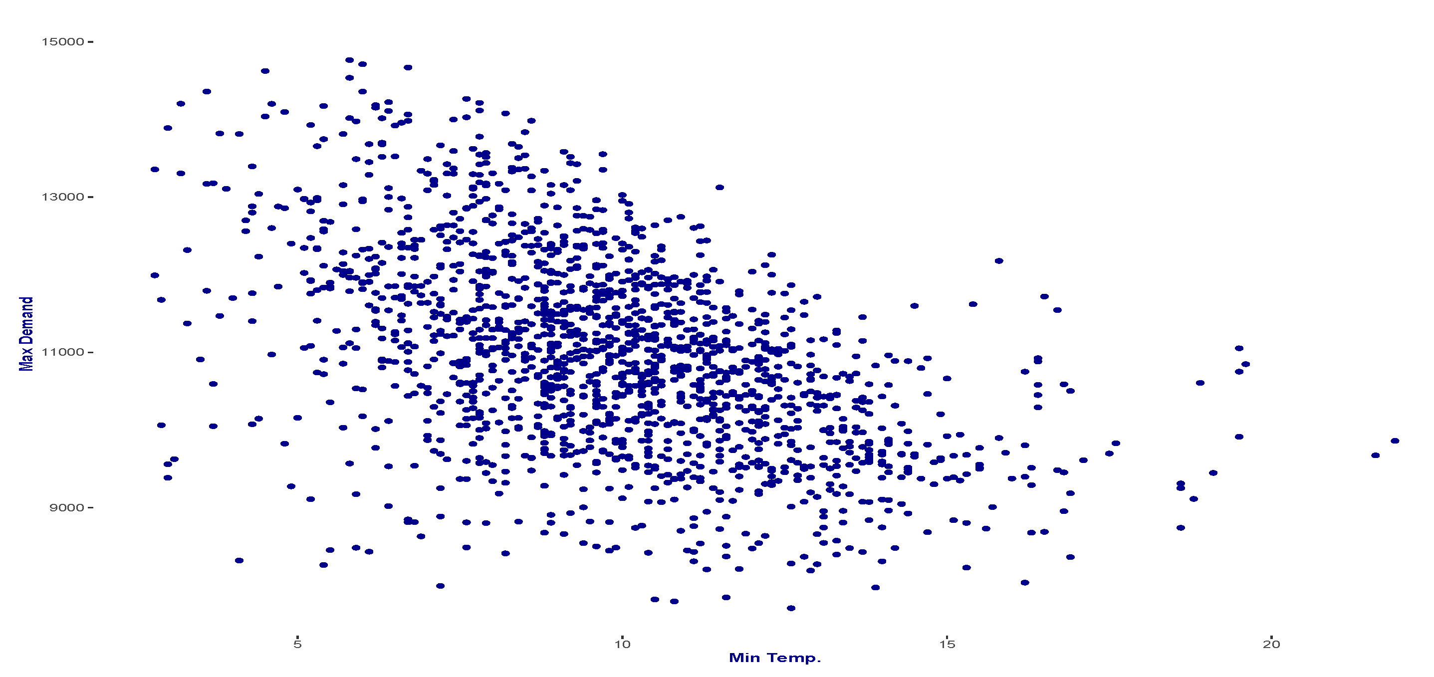
5.1. Data Description

The database we used included daily peak demand and minimum wet temperatures from 1996 to 2022 in Israel. It excludes weekends and holidays when electricity demand is lower. This work focused on the winter season, which occurs in December, January, and February, with a total of 1689 daily observations with a minimum temperature in the range of 2.8 to 21.9 degrees and normalized maximum electricity demand in the range of 7700 MW to 14,700 MW. The scatter diagram in Figure 4 represents the dependence structure between minimum temperature and maximum electricity demand. In

Table 2. Empirical dependence measures.

Pearson’s Correlation	Spearman’s Rho	Gini’s Gamma	Kendall’s Tau	Blomqvist’s Beta
$-0.493$	$-0.500$	$-0.463$	$-0.353$	$-0.34$

, five measures of the strength of the association between the variables are presented.

Following the procedure presented in Section 4.1, the marginal distributions of the two random variables were examined.

Using the Anderson–Darling criterion, the marginals are as follows.

Let X be a random variable representing the daily peak demand in the winter, then the fit distribution is $X\sim Gamma\left(\alpha ,\beta \right):$

$$f_X\left(x\right)=\frac{{\beta }^{\alpha }{e}^{-\beta v}{v}^{\alpha -1}}{\mathsf{\Gamma }\left(\alpha \right)},$$

where $\alpha =79.56$ and $\beta =139.42$. Here, $\alpha >0$ is the shape parameter and $\beta >0$ is the scale parameter.

The fit distribution for the minimum temperature is $Y\sim Logistic\left(\mu ,\sigma \right):$

$$f_Y\left(y\right)=\frac{e^{-\left(u-\mu \right)/\sigma }}{\sigma {\left(1+e^{-\left(u-\mu \right)/\sigma }\right)}^2},$$

where $\mu =9.74$ and $\sigma =1.56$. Here, $\mu$ is the location parameter and $\sigma >0$ is the scale parameter. Figure 5 represents the density functions of the two variables, where the empirical distribution is described by the histogram and the theoretical by the black line. The goodness of fit parameters for both of distributions are shown in

Table 3. Goodness of fit values.

Variable	Distribution	Kolmogorov–Smirnov	Anderson–Darling	p Value
X	Gamma	$0.016$	$0.8143$	$p<0.01$
Y	Logistic	$0.022$	$0.823$	$p<0.01$

.

5.2. The Experiment

By using Equations (14) and (16), the estimated parameters of Gini’s Gamma and Blomqvist’s beta are $\widehat{\mathsf{\Gamma }}=-0.463,$$\widehat{\beta }=-0.34$, respectively. Then, by using the procedure described in Section 4.2, the parameters of the CGG family members are obtained and reported in

Table 4. Estimated parameters of the Clayton generalized Gamma members.

Family	p	a	d
Gamma	1	$0.1$	$8.9$
Standard Gamma	1	1	$1.9$
Wien	1	$0.3$	4
Nakagami	2	$6.4$	$9.9$
Half Normal	2	$10.7$	1
Folded Normal	2	$\sqrt{2}$	1
Rayleigh	2	$9.8$	2
Maxwell–Boltzmann	2	$7.6$	3
Wilson–Hilferty	3	$8.5$	$2.6$
Weibull	$1.7$	10	$1.7$

.

The confidence interval was calculated for each CGG family member and for the Clayton and Gumbel copulas using the method presented in Section 4.3. Figure 6 displays the confidence interval boundaries for each member. The dotted blue represents the upper limit of the confidence interval of the peak demand, and the red dots are the empirical values of peak demand given the minimum temperature.

Note that underestimation occurs when the red dot is above the blue line and overestimation when the red dot is below it. From Figure 6, it can easily be seen that the three family members at the top of Figure 6 fit the upper limit of the probabilistic confidence interval for the relevant range of minimum temperatures below 15 °C. When the temperature exceeds 15 °C, these family members underestimate the peak demand. The rest of the models offer a poorer prediction of the demand, and they all underestimate the peak values for temperatures below 15 °C. The best-fit family member was selected by two fitting measures discussed in Section 4.4.

Table 5. Cost and conditional coverage measures’ values for the CGG family members and Clayton and Gumbel copulas.

Family	$\mathit{CM}$	$\mathit{CC}$
Gamma	$4.9$	$95\%$
Standard-Gamma	$14.3$	$87\%$
Wien	$7.9$	$94\%$
Nakagami	$6.5$	$89\%$
Half Normal	$20.3$	$78\%$
Folded Normal	$85.6$	$55\%$
Rayleigh	$11.3$	$84\%$
Maxwell–Boltzmann	$7.7$	$86\%$
Wilson–Hilferty	$8.5$	$85\%$
Weibull	$8.8$	$87\%$
Clayton	$8.9$	$93\%$
Gumbel	$16.3$	$92\%$

CM values presented in terms of USD 10³.

shows the calculated values of $CC$ and $CM$ for each family member and for the Clayton and Gumbel copulas.

These values are graphically presented in Figure 7.

From Figure 7, it is easy to see that the most appropriate copula function for predicting peak demand using the minimum temperature in the winter season belongs to the Clayton Gamma family member (the orange dot in the figure). This function has the lowest economic loss value and a probability coverage measure closest to $99\%$.

5.3. Major Contributions

∗

The confidence interval of the peak demand based on temperature was estimated, and a probabilistic copula family, the Clayton generalized Gamma, which is comprised of several copula functions and aims at characterizing the dependence structure, was suggested.

∗

This innovative three-parameter family enhances flexibility in adjusting the dependence structure between peak demand and temperature, thus allowing a more accurate estimation of the former.

∗

The superiority of the Clayton Gamma copula over other members of the Clayton generalized Gamma family, as well as popular one-dimensional copulas such as the Clayton and Gumbel copulas was demonstrated in the numerical study provided.

∗

The proposed methodology significantly enriches the number of candidate copulas available for peak demand estimation and, thus, reduces the probability of unmet demand with its dramatic consequences.

6. Conclusions

This work aimed to accurately estimate peak demand, which is one of the fundamental challenges for Independent System Operators responsible for managing power systems. Using temperature, we proposed a probabilistic model to estimate the confidence interval of the peak demand using a new Archimedean family, the Clayton generalized Gamma, comprising several members of copula functions, used to characterize the dependence structure. A conditional value-at-risk $Va{R}_q\left(X\right|Y=y)$ of the daily electricity peak demand $\left(X\right)$ given the daily minimum temperature (Y) was established and used to evaluate the confidence limits of peak demand. Two new measures of the fit were introduced to determine the most appropriate copula: a conditional coverage measure, estimating the proportion of observations covered by the confidence interval, and an economic measure, assessing the economic loss due to an incorrect estimation of peak demand. The latter incorporates a new weight index to better represent the importance of low winter temperatures. Daily data, between 1996 and 2022, in the winter (December–February), were used to examine the proposed methodology. The Clayton Gamma copula member was shown to have the lowest economic loss and the closest conditional coverage to the confidence limit value and is, therefore, the one our study suggests as the most suitable for peak demand prediction. This CGG member clearly provides a more accurate estimate of peak demand, thereby resulting in a system better suited to meet the challenges of climate change. A more accurate estimation of peak demand may require the consideration of several additional variables such as precipitation and radiation intensity. Adding variables requires a higher-dimensional copula and will be the subject of future research.

References

1. Ruth, M.; Lin, A.-C. Regional energy demand and adaptations to climate change: Methodology and application to the state of Maryland, USA. Energy Policy 2006, 34, 2820–2833. [Google Scholar] [CrossRef]
2. Miller, N.L.; Hayhoe, K.; Jin, J.; Auffhammer, M.C. extreme heat, and electricity demand in California. J. Appl. Meteorol. Climatol. 2008, 6, 1834–1844. [Google Scholar] [CrossRef]
3. Parkpoom, S.; Harrison, G.P.; Bialek, J.W. Climate change impacts on electricity demand. In Proceedings of the 39th International Universities Power Engineering Conference, Bristol, UK, 6–8 September 2004; pp. 1342–1346. [Google Scholar]
4. Buys, L.; Vine, D.; Ledwich, G.; Bell, J.; Mengersen, K.; Morris, P.; Lewis, J.T. A framework for understanding and generating integrated solutions for residential peak energy demand. PLoS ONE 2015, 10, e0121195. [Google Scholar] [CrossRef] [PubMed] [Green Version]
5. Narayanan, A.; Morgan, M.G. Sustaining critical social services during extended regional power blackouts. Risk Anal. 2012, 32, 1183–1193. [Google Scholar] [CrossRef] [PubMed]
6. Gerlak, A.K.; Weston, J.; McMahan, B.; Murray, R.L.; Mills-Novoa, M. Climate risk management and the electricity sector. Clim. Risk Manag. 2018, 19, 12–22. [Google Scholar] [CrossRef]
7. Sachdev, M.S.; Billinton, R.; Peterson, C.A. Representative bibliography on load forecasting. IEEE Trans. Power Appar. Syst. 1977, 96, 697–700. [Google Scholar] [CrossRef]
8. Hagan, M.T.; Behr, S.M. The time series approach to short term load forecasting. IEEE Trans. Power Syst. 1987, 2, 785–791. [Google Scholar] [CrossRef]
9. Hong, T.; Fan, S. Probabilistic electric load forecasting: A tutorial review. Int. J. Forecast. 2016, 32, 914–938. [Google Scholar] [CrossRef]
10. Emodi, N.V.; Chaiechi, T.; Alam, B. ABM Rabiul The impact of climate change on electricity demand in Australia. Energy Environ. 2018, 29, 1263–1297. [Google Scholar] [CrossRef]
11. Auffhammer, M.; Baylis, P.; Hausman, C.H. Climate change is projected to have severe impacts on the frequency and intensity of peak electricity demand across the United States. Proc. Natl. Acad. Sci. USA 2017, 114, 1886–1891. [Google Scholar] [CrossRef] [Green Version]
12. Debnath, K.B.; Mourshed, M. Forecasting methods in energy planning models. Renew. Sustain. Energy Rev. 2018, 88, 297–325. [Google Scholar] [CrossRef] [Green Version]
13. Saman, T.; Ali, R. A novel probabilistic regression model for electrical peak demand estimate of commercial and manufacturing buildings. Sustain. Cities Soc. 2022, 77, 103544. [Google Scholar]
14. Lee, G.-C. Regression-Based Methods for Daily Peak Load Forecasting in South Korea. Sustainability 2022, 14, 3984. [Google Scholar] [CrossRef]
15. Fernández-Martínez, D.; Jaramillo-Morán, M.A. Multi-Step Hourly Power Consumption Forecasting in a Healthcare Building with Recurrent Neural Networks and Empirical Mode Decomposition. Sensors 2022, 22, 3664. [Google Scholar] [CrossRef]
16. Lucas Segarra, E.; Ramos Ruiz, G.; Fernández Bandera, C. Probabilistic load forecasting for building energy models. Sensors 2020, 20, 6525. [Google Scholar] [CrossRef]
17. Brusaferri, A.; Matteucci, M.; Spinelli, S.; Vitali, A. Probabilistic electric load forecasting through Bayesian Mixture Density Networks. Appl. Energy 2022, 309, 118–341. [Google Scholar] [CrossRef]
18. Lopez-Martin, M.; Sanchez-Esguevillas, A.; Hernandez-Callejo, L.; Arribas, J.I.; Carro, B. Additive ensemble neural network with constrained weighted quantile loss for probabilistic electric-load forecasting. Sensors 2021, 21, 2979. [Google Scholar] [CrossRef]
19. Ahmed Mohammed, A.; Aung, Z. Ensemble learning approach for probabilistic forecasting of solar power generation. Energies 2016, 9, 1017. [Google Scholar] [CrossRef]
20. Sun, M.; Wang, Y.; Strbac, G.; Kang, C. Probabilistic peak load estimation in smart cities using smart meter data. IEEE Trans. Ind. Electron. 2018, 66, 1608–1618. [Google Scholar] [CrossRef] [Green Version]
21. Ouyang, T.; He, Y.; Li, H.; Sun, Z.; Baek, S. Modeling and forecasting short-term power load with copula model and deep belief network. IEEE Trans. Emerg. Top. Comput. Intell. 2019, 3, 127–136. [Google Scholar] [CrossRef] [Green Version]
22. Kelner, M.; Landsman, Z.; Makov, U.E. Fitting Compound Archimedean Copulas to Data for Modeling Electricity Demand. Int. J. Stat. Probab. 2021, 10, 1–20. [Google Scholar] [CrossRef]
23. Bernards, R.; Morren, J.; Slootweg, H. Statistical modeling of load profiles incorporating correlations using Copula. In Proceedings of the 2017 IEEE PES Innovative Smart Grid Technologies Conference Europe (ISGT-Europe), Turin, Italy, 26–29 September 2017. [Google Scholar]
24. Tian, S.; Huang, W.; Yan, T.; Yang, X.; Fu, Y. Electricity-heat-gas integrated demand response dependency assessment based on BOXCOX-Pair Copula model. IET Energy Syst. Integr. 2022, 4, 131–142. [Google Scholar] [CrossRef]
25. Lin, S.; Liu, C.; Shen, Y.; Li, F.; Li, D.; Fu, Y. Stochastic Planning of Integrated Energy System via Frank-Copula Function and Scenario Reduction. IEEE Trans. Smart Grid 2021, 13, 202–212. [Google Scholar] [CrossRef]
26. Wang, Z.; Xu, X.; Trajcevski, G.; Zhang, K.; Zhong, T.; Zhou, F. PrEF: Probabilistic Electricity Forecasting via Copula-Augmented State Space Model; AAAI: Menlo Park, CA, USA, 2022. [Google Scholar]
27. Chen, B.; Huang, W. Short-Term Load Forecasting Method Based on Copula Correlation Measurement Combined With Attention Mechanism. In Proceedings of the 2021 IEEE 4th International Electrical and Energy Conference (CIEEC), Wuhan, China, 28–30 May 2021. [Google Scholar]
28. Ebrahimi, S.R.; Rahimiyan, M.; Assili, M.; Hajizadeh, A. Home energy management under correlated uncertainties: A statistical analysis through Copula. Appl. Energy 2022, 305, 117753. [Google Scholar] [CrossRef]
29. Kelner, M.; Landsman, Z.; Makov, U.E. New Approach to Multivariate Archimedean Copula Generation. J. Stat. Plan. Inference, 2022; Under Review. [Google Scholar]
30. Genest, C.; Favre, A.-C. Everything you always wanted to know about copula modeling but were afraid to ask. J. Hydrol. Eng. 2007, 12, 347–368. [Google Scholar] [CrossRef]
31. Sklar, M. Fonctions de repartition an dimensions et leurs marges. Publ. Inst. Statist. Univ. Paris 1959, 8, 229–231. [Google Scholar]
32. Joe, H. Multivariate Models and Multivariate Dependence Concepts, 1st ed.; CRC Press: Boca Raton, FL, USA, 1997. [Google Scholar]
33. Kotz, S.; Drouet, D. Correlation and Dependence, 1st ed.; World Scientific: Singapore, 2001. [Google Scholar]
34. Nelsen, R.B. An Introduction to Copulas, 1st ed.; Springer Science & Business Media: Berlin/Heidelberg, Germany, 2007. [Google Scholar]
35. Kelner, M.; Landsman, Z.; Makov, U.E. Compound Archimedean Copulas. Int. J. Stat. Probab. 2021, 10, 126–139. [Google Scholar] [CrossRef]
36. Silva, R.B.; Bourguignon, M.; Cordeiro, G.M. A new compounding family of distributions: The generalized Gamma power series distributions. J. Comput. Appl. Math. 2016, 303, 119–139. [Google Scholar] [CrossRef]
37. Genest, C.; Nešlehová, J.; Ben Ghorbal, N. Spearman’s footrule and Gini’s Gamma: A review with complements. J. Nonparametric Stat. 2010, 22, 937–954. [Google Scholar] [CrossRef]
38. Nelsen, R.B. Concordance and Gini’s measure of association. J. Nonparametric Stat. 1998, 9, 227–238. [Google Scholar] [CrossRef]
39. Blomqvist, N. On a measure of dependence between two random variables. Ann. Math. Stat. 1950, 21, 593–600. [Google Scholar] [CrossRef]
40. Genest, C.; Rivest, L.-P. Statistical inference procedures for bivariate Archimedean copulas. J. Am. Stat. Assoc. 1993, 88, 1034–1043. [Google Scholar] [CrossRef]
41. Frees, E.W.; Valdez, E.A. Understanding relationships using copulas. N. Am. Actuar. J. 1998, 2, 1–25. [Google Scholar] [CrossRef]
42. Durrleman, V.; Nikeghbali, A.; Roncalli, T. Which Copula Is the Right One; Researchgate: Berlin, Germany, 2020. [Google Scholar]
43. Najafi, M.; Akhavein, A.; Akbari, A.; Dashtdar, M. Value of the lost load with consideration of the failure probability. Ain Shams Eng. J. 2021, 12, 659–663. [Google Scholar] [CrossRef]
44. Van Der Welle, A.; Van Der Zwaan, B. An Overview of Selected Studies on the Value of Lost Load (VOLL); Energy Research Centre of the Netherlands (ECN): Petten, The Netherlands, 2007. [Google Scholar]
45. Heinrich, C.; Ziras, C.; Jensen, T.V.; Bindner, H.W.; Kazempour, J. A local flexibility market mechanism with capacity limitation services. Energy Policy 2021, 156, 112335. [Google Scholar] [CrossRef]
46. Schmalensee, R. Competitive Energy Storage and the Duck Curve. Energy J. 2022, 43. [Google Scholar] [CrossRef]
Figure 1. The statistical process.
Energies 15 06081 g001
Figure 2. Clayton–Wien member of the CGG family.
Energies 15 06081 g002
Figure 3. Power exponential linear weight for different values of k.
Energies 15 06081 g003
Figure 4. Max. electricity demand vs. Min. wet temperature.
Energies 15 06081 g004
Figure 5. Density of Min. temperature and Max. electricity demand.
Energies 15 06081 g005
Figure 6. Lower confidence interval (orange dashed line) and upper confidence interval (blue dashed line) for members of the CGG family.
Energies 15 06081 g006
Figure 7. Fitting measures for the CGG members and Clayton and Gumbel copulas.
Energies 15 06081 g007