Article

Control of Heat Transfer in a Vertical Ground Heat Exchanger for a Geothermal Heat Pump System

Department of Electrical and Computer Engineering, School of Engineering and Computer Science, Oakland University, Rochester, MI 48306, USA
*
Author to whom correspondence should be addressed.
Energies 2022, 15(14), 5300; https://doi.org/10.3390/en15145300
Submission received: 15 June 2022 / Revised: 9 July 2022 / Accepted: 18 July 2022 / Published: 21 July 2022
(This article belongs to the Topic Geothermal Energy Technology and Current Status)

Abstract

:
This paper presents a mathematical model of heat transfer behavior between the liquid inside vertical underground geothermal pipes and the surrounding ground for heating (in the winter) and cooling (in the summer) modes in a ground heat exchanger (GHE) that can optimize its output temperature. The GHE’s output temperature reaches the appropriate value when the water velocity is lowered enough. Subsequently, the proposed model was applied to a case study of a 400-ton geothermal heat pump system (GHPS) at Oakland University, in both the heating and cooling modes, to assess its validity and improve the GHE’s performance. The model was implemented in MATLAB using an ordinary differential equation (ODE) solver. Four different water velocities were used to demonstrate the significant effect of velocity on the loop exit temperature. Model predictive control (MPC) was designed to optimize the GHE’s output temperature by controlling the water velocity, which could reduce the energy consumption used for heat and water circulating pumps. The results reveal that the acceptable range of the water velocity for Oakland University’s GHE was between 0.35 and 0.45 m / s , which ensured that the heat pump system delivered the proper temperature to provide the Human Health Building (HHB) with a comfortable temperature regardless of the season. The suggested water velocity ranges in vertical single U-tube pipes with diameters of De 25 mm , De 32 mm , and De 40 mm are between 0.33 and 0.43 m / s , 0.35 to 0.45 m / s , and 0.38 to 0.48 m / s , respectively.

1. Introduction

To take advantage of the existing heat contained within the earth, an efficient technology known as the geothermal heat pump system (GHPS) was proposed. GHPSs were developed to efficiently heat and cool buildings by harnessing this energy from the earth. Thus, the GHPS provides high-efficiency heating and cooling for buildings, as well as domestic hot water production that can be used in different applications (electricity production, greenhouse, etc.). The heating and cooling efficiencies of the GHPS outperform conventional heating and air conditioning systems, which are 30% to 70% higher than conventional heating, and 20% to 50% higher than air conditioning systems. Furthermore, the GHPS significantly reduces electricity use by approximately 75% in compassion to conventional heating or cooling systems [1]. It would be best if renewable energy sources were used to meet GHPSs’ power needs instead of electricity. Energy efficiency attained with this GHPS technology will have significant environmental benefits, such as decreased carbon dioxide ( CO 2 ) emissions and a quieter atmosphere. Therefore, the GHPS is considered a clean, reliable, renewable, and sustainable source of energy that requires very low maintenance and is unaffected by climatic conditions. It is also environmentally friendly and greatly reduces CO 2 emissions by up to 52% when compared to heating, ventilation, and air conditioning (HVAC) [1,2,3,4,5,6]. After incurring initial installation costs, GHPS is free to operate. Since there are few restrictions for GHPS applications, it can be installed virtually anywhere and operated continuously for both heating and cooling purposes to provide the building with a comfortable temperature regardless of the weather. Additionally, as the GHPS benefits from more heat energy, it would be best to install its ground heat exchanger (GHE) in an area with high thermal conductivity, preferably moist soil. The GHPS was first used in North America less than one hundred years ago and is now gaining popularity globally, especially in colder regions, because of its high energy efficiency and thus lower operating cost compared to conventional systems [7]. Additionally, countries utilizing GHPS aim to create environments with a low-carbon economy by reducing CO 2 emissions. It should be highlighted that regular monitoring and control are necessary to keep the system operating at optimum efficiency. On the other hand, despite all the benefits of the GHPS, its installation is expensive due to the high cost of drilling boreholes if the design is vertical, and it requires a large land area if the design is horizontal [8]. In addition, its initial capital cost is significant, roughly 30–50% higher than traditional heating and air conditioning systems [9]. For these reasons, the GHPS is not used as widely as it could be if it were cheaper to install. To compensate for the high installation costs, researchers have conducted numerous studies to increase the GHPS’s efficiency and to make the system more reliable and affordable for household use. Ultimately, due to its high efficiency, the GHPS pays for itself in the long term.
The ground heat exchanger (GHE) is a crucial component of the GHPS and plays a key role in utilizing the earth’s heat energy by exchanging heat with the ground due to its actual contact. Most benefits from the earth’s thermal energy can be attained when the GHE is well-designed, including in terms of configuration, installation location, borehole heat exchanger capacity, and performance factors, which ensure that the GHE’s output temperature reaches the ground temperature. Thus, improvements should emphasize GHE characteristics, as any improvement will benefit from the overall GHPS efficiency and result in a lower initial capital cost.

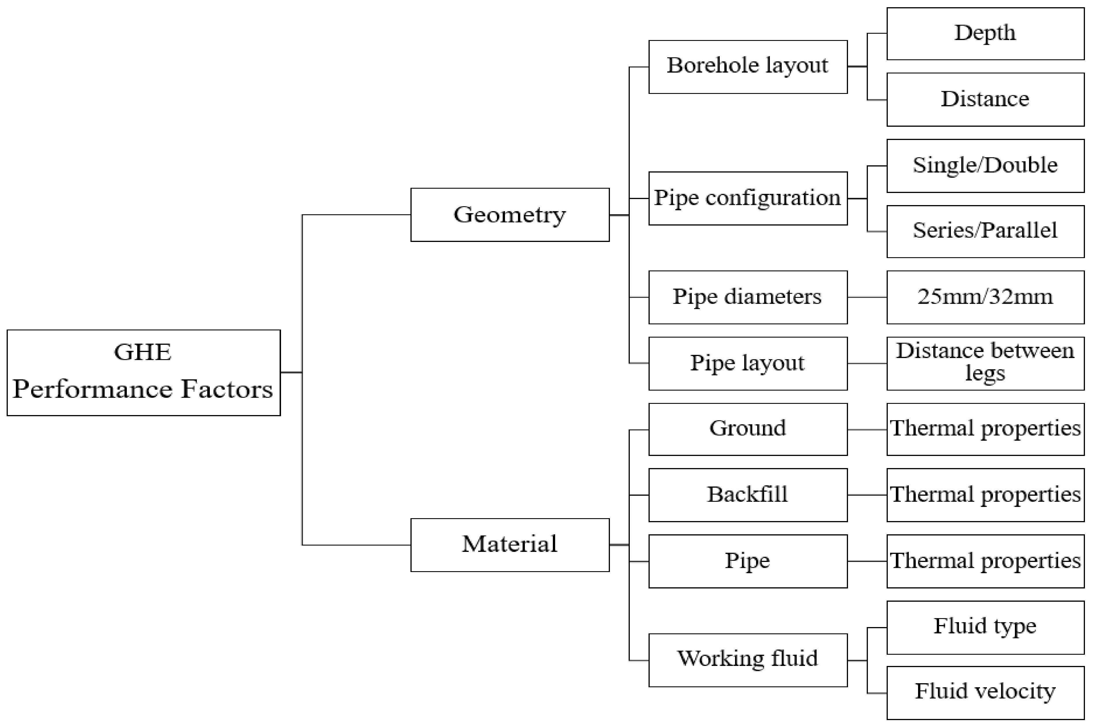
2. GHE Performance Factors

Many factors can affect the vertical GHE’s performance, such as the soil type, backfill material thermal conductivity, pipe’s material thermal conductivity, borehole depth, the distance between two boreholes, shank spacing between the pipes, and working fluid and its velocity in the U-tube pipe, as shown Figure 1.
For instance, each soil type has a different thermal conductivity that is determined by its physical component properties. When the thermal conductivity of the soil material is high, it indicates that it is fully saturated, and its thermal resistance is therefore low, allowing heat to flow through its layers quickly. Conversely, when its thermal conductivity is low, it indicates that the soil material is unsaturated, and its thermal resistance increases, slowing the heat flow. Therefore, its thermal conductivity is dependent on its saturation level [10]. Wang et al. [11] evaluated the thermal conductivity of different soil types, including loam, clay, and sand, using the improved ‘de V-1’ model. The results revealed that the sand performed better than loam and clay soils in terms of thermal conductivity and heat diffusion. Moreover, Wang et al. [11] agreed with Tang and Hossein [12] that sand performed better than clay. Therefore, the soil’s high thermal conductivity is essential for use in either installing the GHE or as a backfill material to have a suitable design for GHE.
Following the installation of the U-tube pipe, the space between the pipe and the borehole wall is filled with conventional backfill materials, including bentonite mixed with sand and cement with the amount of water which depends on the mass ratio of each material component. These materials have the advantages of being extremely durable, swelling-capable, and impermeable, but their thermal conductivities are low. Depending on the type of surrounding soil, engineers vary the ratio of each material in the mixture to best suit the environment. Therefore, the boreholes must be completely grouted to ensure that the grout fills the borehole without any air gaps, which can cause thermal discontinuity (called contact resistance). That will create a strong thermal connection between the U-tube GHE pipe and the ground, which increases the heat transfer capacity. It also keeps the borehole wall from collapsing [13].
To maintain the GHE’s efficiency in coastal regions, Lee et al. [14] suggested utilizing bentonite that contains a substantial quantity of montmorillonite. Furthermore, Lee et al. [15] recommended using cementitious backfill material in dry soil due to its good desiccation and shrinkage properties. Shadley and Den Braven [16] tested several backfill mixtures and pure materials and then compared them to a standard bentonite backfill material. Experimental results of the backfill material test showed that the highest thermal conductivity was found to be in saturated natural sandy soil. Table 1 demonstrates the soil material properties [17].
The backfill material is regarded as a heat transfer medium between the GHE and the soil; thus, it has a high thermal conductivity to fulfill heat transfer into directions. The pure backfill material will have a thermal conductivity ranging from 0.8 W/m·K to 2.4 W/m·K, but when mixed with other soils, it could be as high as 2.6 to 3.5 W/m·K [14,18,19]. Dehkordi and Schincariol [20] demonstrated that increasing the thermal conductivity of backfill material has a positive impact on heat extraction. Thus, they pointed out that by using the high thermal conductivity of the backfill material (3 W/m·K), heat extraction can be increased by more than 10% in comparison to the low thermal conductivity of the backfill material (1 W/m·K). Additionally, increasing the backfill material’s thermal conductivity could reduce the thermal gradient between the pipe and the surrounding ground, which increases the efficiency of the heat exchange rate [20]. Alberti et al. [21] compared the thermal conductivities of three different backfill materials. The results showed that the thermal resistance of the first and second boreholes backfilled with 2.3 W/m·K was lower than the thermal resistance of the third borehole backfilled with 0.7 W/m·K, with thermal resistance result values of 0.054 m·K/W, 0.054 m·K/W, and 0.1354 m·K/W, respectively. For instance, the use of high thermal conductivity backfill materials could increase the borehole surface temperature and reduce thermal borehole resistance [22]. This results in rapid heat transfer between the fluid inside the pipe and its surrounding grounds and can shorten the length of the GHE pipe. Thus, the GHPS’s initial capital and operating costs are reduced. This becomes more important in the double U-tube borehole configuration than in the single U-tube borehole configuration. Zhang et al. [23] demonstrated the influences of the backfill material’s thermal conductivity on the GHE’s four different U-tube pipe sizes and configurations, namely as double U-tube 32, double U-25, single U-32, and single U-25. They concluded that the heat thermal conductivity of the backfill material has the highest influence on reducing the GHE pipe’s length in a double U-32, followed by double U-25, single U-32, and single U-25.
The pipe acts as a heat transfer interface between two mediums, namely, the working fluid inside the pipe, and its surrounding grounds. The pipe should have durability, flexibility, and longevity to resist wear, leaks, and other damage; to be simple to install; and for cost-effectiveness [24]. Furthermore, the pipe’s material should have a high thermal conductivity to promote the heat transfer process. It is important to note that the thermal conductivity of the pipe material influences heat transfer performance, which in turn can enable heat to flow in either direction. Most geothermal ground heat pump system projects use a high-density polyethylene (HDPE) pipe because of its durability, flexibility, longevity, and low cost, despite its conductivity being lower than metal pipe. The pipe’s material thermal conductivity ranges from 0.35 W/m·K to 0.49 W/m·K, and its lifespan is up to approximately 50 years [25]. Therefore, more improvements in manufacturing characteristics are needed to increase its thermal conductivity, which could improve the GHE’s performance. For instance, Bassiouny et al. [26] mixed miniature aluminum wires with a conventional HDPE pipe material. They found that when an additional 2 mm of aluminum wire was added to the material of the pipe itself, the thermal conductivity rose 25%; when an additional 3 mm of aluminum wire was added to the material of the pipe itself, the thermal conductivity rose 150%, when compared to the original HDPE pipe. In addition, Raymond et al. [27] incorporated some additives into the polymer resin in the original HDPE pipe extrusion. The result demonstrated that the enhanced pipe material’s thermal conductivity increased by 75%, from 0.4 W/m·K to 0.7 W/m·K, as compared to the original HDPE pipe. The results also showed that this improvement reduced the thermal resistance of the borehole by 24%. Moreover, Bouhacina et al. [28] added longitudinal fins to the original HDPE pipe’s inner surface. The new design pipe was able to increase heat extraction by approximately 7% in comparison to the original pipe. Therefore, increasing the thermal conductivity of the pipe material could bring some advantages, such as reducing borehole thermal resistance, decreasing pipe length, increasing heat extraction from the ground, and either heating or cooling the water leading to lower initial installation costs.
As the borehole gets deeper, more heat transfer occurs until it reaches a point where it loses more heat than it gains. At that point, when the difference between the ground and fluid temperature decreases, the heat transfer efficiency will relatively decrease, and the borehole drilling cost will significantly rise. In the GHPS’s engineering design, increasing the borehole depth does not bring greater benefits than improving other parameters such as increasing the thermal conductivity of backfill material; this can be satisfied with the existing borehole depth if it provides adequate heating energy. Moreover, increasing the borehole depth lengthens the period of water circulation, requiring more energy to circulate the water within the loop. Given this, Song et al. [29] suggested that to limit heat loss, the borehole should not be too deep; thus, the depth for a single U-tube would be roughly 80 m. Furthermore, the depth of the borehole for double U-25 is between 80 m and 100 m, whereas the depth of the borehole for double U-32 is between 90 m and 110 m [8]. Zeng et al. [30] compared two borehole thermal resistances for double U-tube and single U-tube borehole configurations. The result showed that the double U-tube borehole had better performance than a single U-tube borehole since its thermal resistance was reduced by 30–90% when compared to the single U-tube borehole thermal resistance. Therefore, more heat transfer efficiency in the GHE can be attained when the double U-tube configuration is connected in parallel rather than in series [30]. Furthermore, the multi-U-tube borehole configuration outperforms the double and single U-tube borehole configurations [31].
It is also worth noting that the distance between two boreholes is crucial, as it has a significant impact on the borehole’s thermal resistance. Enough space must be left between them to prevent any thermal interference as it affects the performance of the GHE. The thermal interference is measured by the distance between two boreholes; if the distance is less than what is suggested for the GHE pipe installation design, there will be more thermal interference between them. However, if the distance is too large, more land area is required to install the GHE, and an additional pipe network is required for connections between boreholes pipes, which will increase the initial capital cost. Therefore, this distance should be neither too small nor too large. Gultekin et al. [32] concluded that the distance between two U-tube boreholes should be between 4.5 m and 6 m. Moreover, they agreed with another study [33] that 5 m is the optimum separation between two borehole walls.
Another factor that influences heat transfer performance in the GHE is the shank spacing between two legs of U-tube pipes, which causes a thermal short circuit phenomenon when the legs of the U-tube pipes are in contact or extremely close to each other [34]. If there is not enough space, the probability of thermal short-circuiting increases, making heat transfer inefficient. To prevent a thermal short circuit and enhance heat transfer in the GHE between the U-tube pipe and its surroundings, the U-tube pipe must be centrally located in the borehole with precise space between them. Interestingly, shank separation of less than 60 mm between U-tube pipes will cause a thermal short circuit, and the heat transfer deteriorates [35]. However, if the space is raised to 60 mm, a thermal short circuit will not occur [36]. In addition, it could be stable if the shank spacing is larger than 90 mm [12]. Furthermore, Zheng et al. [33] determined that the ideal spacing between two U-tube pipes is between 100 mm and 200 mm.
The working fluid acts as a heat transfer carrier between the heat pump and the ground; it has high thermal conductivity, heat capacity, and the lowest viscosity because it affects the convective thermal resistance (between the fluid in the U-tube and the ground) [37]. Dada and Benchatti [38] evaluated three different working fluids—water, gasoline, and glycol. According to their findings, utilizing water as a working fluid could store and recover more thermal heat energy than other working fluids. Pure water has been employed as a heat-carrying fluid in many GHPS systems since their inception for cooling and heating processes due to its high ability to absorb and store heat from the ground and low cost, but its applications have limited antifreeze properties. In cold climates, pure water could be mixed with antifreeze to prevent it from freezing, which would improve heat transfer in GHE. When antifreeze is mixed with the working fluid, the volume concentration must be exact. If the concentration is not in the proper proportion, it could affect the convective thermal resistance, which in turn can affect the GHE’s heat transfer performance. For instance, adding 33% ethanol to 67% pure water increases the kinematic viscosity, decreases the water’s thermal conductivity, and increases the convective thermal resistance, affecting the water–ground heat exchange. However, if the proportion is reduced to 20%, it could enhance the working fluid’s physical properties, maximizing the heat transfer between water and its surrounding grounds [39]. Tang and Nowamooz [12] concluded that adding 24% ethanol to the working fluid outperformed adding 20% CaCl2, 25% propylene glycol, and 33% propylene glycol, respectively, to the working fluid. Recently, GHPS’s engineer designers have turned to using nanofluids as working fluid due to the obvious improvement in the convective heat transfer coefficient [40,41]. Narei et al. [42] concluded that employing an Al2O3/water nanofluid as a working fluid could decrease the borehole length of a single U-tube configuration by 1.3% when compared to pure water. Nanofluid technology is still relatively new for use as a working fluid in GHS systems; hence, more research (both theoretical and empirical) should be considered.
Other studies examined how the fluid velocity within the pipe affected the heat transfer performance of the GHE. Zhou et al. [8] assessed the influence of varying water velocities through various vertical ground heat exchanger pipes, namely, single U-32, double U-25, and double U-32, on heat transfer performance. The results showed that the appropriate water velocity ranges for single U-32 are between 0.4 and 0.6 m/s, 0.4 and 0.5 m/s for double U-25, and 0.3 and 0.4 m/s for double U-32. In addition, Li et al. [43] suggested that the water velocity range for a single U-tube should be between 0.4 m/s and 0.7 m/s for maximum efficiency. Wang et al. [44] demonstrated the impacts of water velocity on the heat transfer efficiency of deep borehole heat exchangers (DBHE) with a depth of 2000 m using a developed numerical model. They examined water velocities ranging from 0.04 m/s to 1.3 m/s and found that a higher heat exchanger rate and a maximum output temperature can be attained when the water velocity is between 0.3 m/s and 0.7 m/s. Another study by You et al. [45] used three different water velocities of 0.26 m/s, 0.51 m/s, and 1.02 m/s to demonstrate the influences of circulating water velocity on the heat exchanger rate, where the water temperature inside the pipe remained constant at 35 through the operational test. Their results indicated that the heat exchanger rates were found to be 84 W/m, 116 W/m, and 94 W/m, when the water velocities were 0.26 m/s, 0.51 m/s, and 1.02 m/s, respectively. The maximum heat exchanger rate was achieved when the water velocity was 0.51 m/s; however, the heat exchanger rate decreased when the water velocity was raised to 1.02 m/s. Therefore, the appropriate water velocity was between 0.5 m/s and 0.6 m/s. From this, it can be concluded that the heat exchanger rate per meter increases with water velocity until it exceeds the allowable range of water velocities, at which point the heat exchanger rate decreases. Additionally, You et al. [45] agreed with another study [12] that the optimal water velocity is around 0.5 m/s. Interestingly, Casasso and Sethi [46] demonstrated that optimizing the water velocity can reduce the borehole’s thermal resistance, which can maximize the heat transfer in either direction. According to the findings of these studies, the water velocity should be in an acceptable range, that is neither too high nor too low, to promote better heat transfer and achieve the desired temperature. When the water velocity is too high, more energy is required to circulate the water, but more importantly, the exit temperature from the loop is not different enough from the entrance. When the flow velocity is too low, the heat transfer is decreased, and the water temperature reaches the ground temperature well before the exit, rendering most of the loop useless. Optimally, one would control the velocity such that the exit temperature is the same as the ground and that the entire loop is utilized equally.
Implementing the suggestions mentioned in the GHE’s performance factors section could increase the GHE’s thermal performance to reach the appropriate loop exit temperature. However, further improvements are required to increase its performance. For example, circulating fluid through a U-tube pipe consumes energy, which will increase with higher velocities; hence, controlling the fluid velocity is critical. Therefore, in this paper, we propose a mathematical model of heat transfer behavior between the fluid inside the vertical underground pipes and the surrounding ground in a ground heat exchanger for heating and cooling modes. Model predictive control (MPC) is designed to optimize the GHE’s output temperature by controlling the water velocity.
The rest of the paper is arranged as follows: Section 3 contains the heating and cooling modes. A mathematical model of heat transfer behavior between the fluid in a single vertical underground U-tube pipe and the surrounding ground is presented in Section 4. Section 5 provides a bilinear state–space model, linearization, and discretization. Section 6 presents the MPC design. An experimental GHPS case study is presented in Section 7. Section 8 presents the results and discussion. Section 9 provides a brief conclusion.

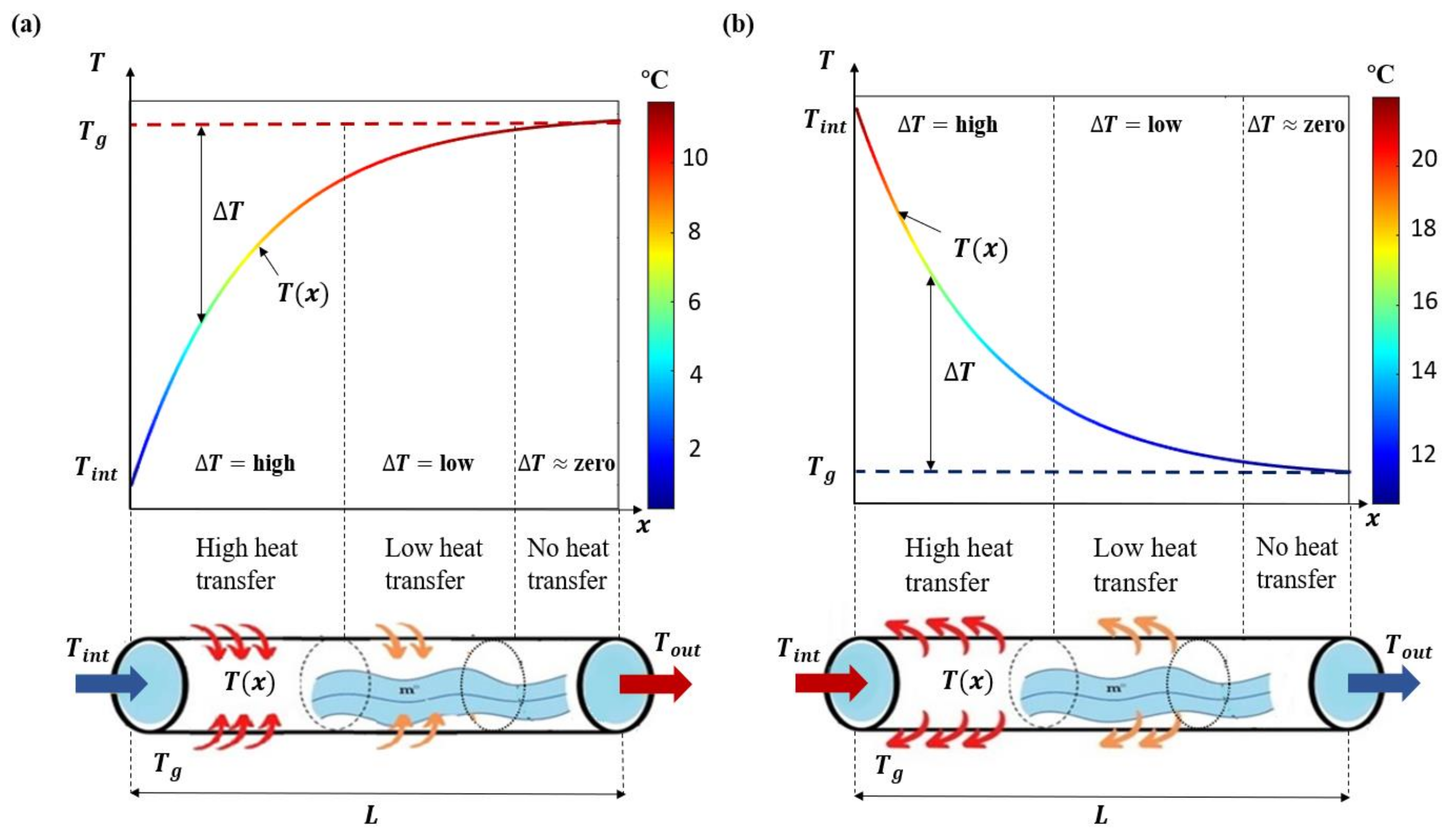
3. Heating and Cooling Modes

The heat transfer mechanism between the circulating water inside the vertical U-tube pipe and the surrounding grounds is as follows: through conduction, the heat transfers from the grout to the outer pipe wall and from the outer to the inner pipe wall, and by convection from the inner pipe wall to the circulating water. The GHPS operates in the heating mode when the ground temperature is higher than the ambient air temperature. The heat transfer profile between the fluid inside the vertical underground pipes and the surrounding ground in a ground heat exchanger for the heating mode is presented in Figure 2a. The temperature difference along the pipe is expressed as Δ T = T g T x . Here, T g represents the ground temperature, while T x is the water temperature. Based on the Δ T value, the heat transfer process can be classified as either high heat transfer, low heat transfer, or no heat transfer. At the beginning of the pipe ( x = 0 ), the heat transfer flows rapidly from the ground to the water inside the pipe because of the significant (∆T) temperature difference. The water temperature, T x , will continue to rise as the water flows through the pipe, and ∆T will drop. The low heat transfer occurs when the water temperature is about to approach the ground temperature, which typically occurs before the pipe’s exit. The water temperature profile, T x , barely varies by the end of the pipe ( Δ T 0 ) if the water velocity is not too high and if other system parameters are in good condition for thermal conductivity. Therefore, it can be regarded as reaching the ground temperature. When in the heating mode, the system can benefit from the maximum heat in the ground when the water temperature reaches the equilibrium point. When in the cooling mode, the system works in reverse. Figure 2b demonstrated the heat transfer profile in the GHE for the cooling mode. In this case, the temperature difference Δ T was calculated as Δ T   = T x T g . As the water reached ground temperature, the heat in the water was transferred to the ground. Further numerical example explanations are presented in Section 8.

4. The Heat Transfer Model

4.1. Model Assumptions

To study the heat transfer behavior in a vertical single U-tube configuration of GHE, some assumptions are made as follows:
Steady-state.
The heat transfer is one-dimensional, modeled in the x-direction only.
Heat is transferred through conduction between the soil and outside the pipe wall (in cylindrical coordinates); heat is transferred through convection in the fluid inside the pipe.
The area surrounding the outside pipe wall (the borehole wall and grout soils) is treated as a single medium with a single thermal resistance, R v .
Three thermal resistances are considered as follows:
-
R g r o u n d : resistance of the ground.
-
R w a l l : resistance of pipe wall.
-
R c o n v : resistance of water in the pipe.
The ground temperature (borehole wall and grout soils surrounding the out-pipe wall) is assumed to be at 11.6   during both heating and cooling modes (the loop is below the frost line).
Flowing groundwater does not affect heat transfer.

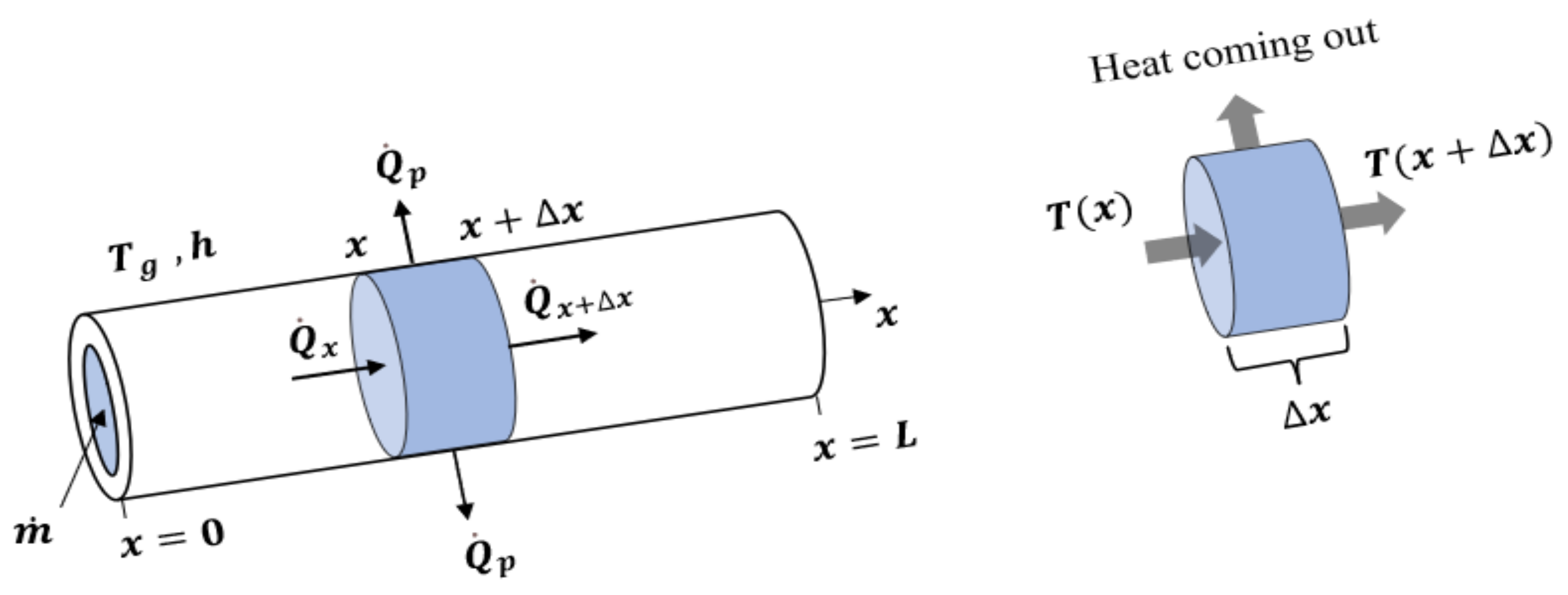
4.2. Governing Equations

A mass flow rate of water flowing in only one direction inside an underground pipe can be calculated using m ˙ = ρ v A , where ρ is the density of the fluid, v is the velocity of the working fluid, and A is the cross-sectional area of the pipe. Q ˙ x is heat flow in at position x, Q ˙ x + Δ x is heat flow out at x + Δ x , and Q ˙ p is the heat coming out of the water to the ground, as shown in Figure 3.
The conservation of energy equation was used to model the heat transfer that can be conducted through the pipe from x to Δ x . The conservation of energy equation is
E s t = Q ˙ + W ˙ s + Σ m ˙ h + 1 2 v + y z i Σ m ˙ h + 1 2 v + y z o ,
where E is the system energy, W s is the system work done (all types of work other than flow work), Q is the rate of heat transfer, m ˙ is the mass flow rate of the water, v is water velocity, and t is the time. The total rate of heat transfer is expressed as
Q ˙ = Q ˙ x Q ˙ x + Δ x Q ˙ p
Substituting the total rate of heat transfer into Equation (1), implementing the assumptions in Section 4.1, and replacing i ,   and o with x and x + Δ x , respectively, renders
0 = Q ˙ x Q ˙ x + Δ x Q ˙ p + m ˙ h x h x + Δ x .
Conduction in the direction of the flow in Equation (3) can be expressed in terms of temperature by utilizing Fourier’s model; thus,
Q ˙ x = k T x x ,   Q ˙ x + Δ x = k T x x + Δ x ,
where k is the fluid thermal conductivity. The Newton’s Law of Cooling equation is used to calculate the rate of convective heat transfer from the water to the pipe’s wall [47]. The heat exchanger Q ˙ p , between the water and the ground temperature is calculated as follows:
Q ˙ p = U 0 A 0 T x T g ,
where A 0 is the pipe’s surface area, which equals A 0 = P 0 Δ x , U 0 is overall heat transfer coefficient, T x is the temperature, T g is the ground temperature, and P 0 is the outside periphery of the pipe. Substituting Q ˙ x , Q ˙ x + Δ x , and Q ˙ p into Equation (3) results in the following:
0 = Q ˙ x Q ˙ x + Δ x U 0 P 0 T x T g d x + m ˙ h x h x + Δ x .
Integrating Equation (6) from x to x + Δ x yields
0 = x x + Δ x f q x d A x x + Δ x f q   x + Δ x d A x x + Δ x U 0 P 0 T x T g d x + m ˙ h x h x + Δ x
where
f q x = k T x x , f q x + Δ x = k T x x + Δ x ,   and   h x h x + Δ x C p T x T x + Δ x .
By substituting the integration limits for these f q x , and f q x + Δ x , we obtain f q x + Δ x f q x , as provided below:
0 = k A T x x + Δ x k A T x x x x + Δ x U 0 P 0 T x T g d x m ˙ C p T x T x + Δ x  
Dividing Equation (8) by Δ x , and then substituting the mass flow rate of water, m ˙ = ρ v A , and the limit is taken as Δ x 0 . These yield in the case of constant properties and cross-sectional area the following:
0 = k A 2 T x 2 U 0 P 0 T T g ρ v A c p T x
The heat equation is presented in Equation (9), a second-order ordinary differential equation. The first term is heat conduction, the second is the rate of heat transfer to the ground, and the third is fluid convection. Dividing Equation (9) by A gives
k 2 T x 2 = U 0 P 0 A T T g ρ v C p T x
where P o = π d o L , and A = π 4 d i 2 . By substituting these into Equation (10), we obtain the heat transfer equation as follows:
k 2 T x 2 = 4   U 0 L d 0   d i 2 T T g ρ v C p T x

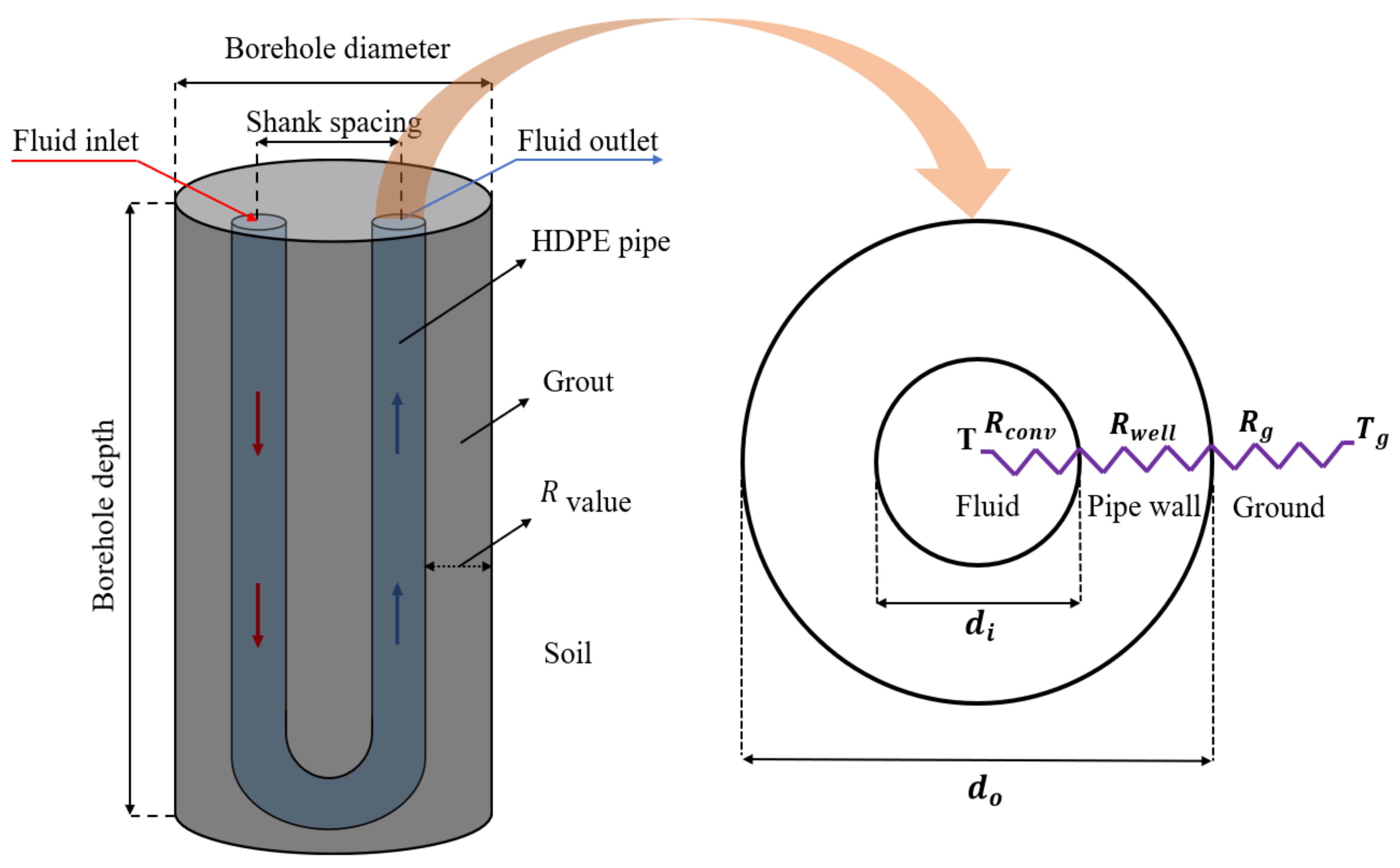
4.3. Thermal Resistance Network

Three thermal resistances in series are considered when transferring heat from/to the ground to/from the fluid inside the pipe, respectively. As discussed in the GHE performance factors section, these resistances have an impact on GHE performance, which is dependent on the thermal conductivity of the soil, pipe wall material, and working fluid. The thermal resistances are exterior convection resistance, conduction thermal resistance, and internal convection resistance, as shown in Figure 4.
By using the thermal resistance method, the total thermal resistance equals the sum of the three thermal resistances since they are in series. Therefore, the total thermal resistance is expressed in Equation (12):
R T H = 1 h i A i + ln d 0 d i 2 π k L + R g
Multiplying Equation (12) by A 0 A 0 gives
R T H = 1 h i A 0 A i 1 A 0 + A 0 ln d 0 d i 2 π k L A 0 + R g A 0 A 0
Extracting A 0 from Equation (13) to obtain the R-value yields
R T H A 0 = 1 h i A 0 A i + A 0 ln d 0 d i 2 π k L + R g A 0
Simplifying in terms of diameter,
R T H A 0 = 1 h i d 0 d i + d 0 ln d 0 d i k + R g 2 π d 0 L
Heat convection occurs when heat is transferred through the movement of a liquid or gas rather than through a solid object. When temperature differences between the water and pipe’s wall are substantial, heat convection can be enhanced. The convective heat transfer coefficient is h i , and its units are W m 2 ° . The heat transfer convection coefficient, which is the most critical parameter in the heat transfer process, is affected by the velocity of the fluid and its natural motion, and the difference in temperatures. The Dittus–Boelter Equation was used to compute the convective heat transfer coefficient as presented in Equation (16) [48].
N U d i = 0.023   P r n R e d i 0.8
N U d i is the Nusselt number that equals h i d i k w , P r is the Prandtl number that equals µ   C p   k w , and R e d i is the Reynolds number of circulating fluid that equals ρ   v   d i µ . h i is the convection heat transfer coefficient between the water and the pipe wall, d i is the pipe inner diameter, v is the water velocity, k w a t e r is the thermal conductivity of the water (calculated at the film temperature), µ is the dynamic viscosity, and c p is the specific heat. Here, n depends on the weather. In the winter, when GHPS is to be used for heating, the circulating fluid temperature is lower than the ground temperature, and the exponent of heating n = 0.4 . However, in the summer, GHPS is in its cooling mode, the fluid temperature is higher than the ground temperature, and the exponent of cooling n = 0.3 . Substituting N U d i , P r , and R e d i into Equation (16), the convective heat transfer coefficient is obtained:
h i = k w a t e r d i 0.023 µ   C p k w a t e r n ρ   v   d i µ 0.8
The overall heat transfer coefficient, U 0 , measures how much heat transfers through these three series resistances. This means that when the U 0 is large, heat is transferred from the hot region to the cold at a higher rate. The following equation describes how to calculate the overall heat transfer coefficient U 0 :
U 0 = 1 h i d o d i + d o   l n d o d i k p + R v 1
where 1 h i d o d i represents the R-value of water convection inside the pipe, d o   l n d o d i k p i p e represents the pipe wall conduction R-value, and R v represents the ground resistance R-value. As was assumed earlier in the model assumption in Section 4.1, the ground and grout regions are treated as a single thermal medium with the same singular resistance known as R v , and its units are (m2·°C)/W.
It can be seen from Equation (18) that the overall heat transfer coefficient U 0 is inversely proportional to the sum of R-values of the heat transfer components. Because the pipe wall has the lowest thermal conductivity in contrast to soil and water, it can act as a physical barrier that can reduce heat transfer between the ground and fluid inside the pipe, but that is mitigated with a relatively small wall thickness.
As a result, we have the steady-state heat transfer equation in its final form, which is a nonlinear second-order ordinary differential equation:
k 2 T x 2 = ρ v c p T x 4 d o d i U 0 T T g

5. Bilinear State Space Model

The GHE’s heat transfer process between the water inside the pipe and the surrounding ground balances the water velocity with the exit temperature, where the water velocity is an input control variable, the ground temperature is a disturbance to the system, and the exit temperature is an output of the system. Due to the flow of water inside the pipe at varying velocities, and the heat transfer dynamic between the water inside the pipe and the surrounding ground, the system has nonlinear characteristics. This type of nonlinearity is known as a bilinear system (BLS), and it occurs when the system’s dynamic behavior is affected by a process or an unmeasured disturbance. The behavior of a bilinear system can be found in a variety of applications, including chemical processes, physics, and thermal energy. For instance, in GHE, the heat transfer process is affected by the working fluid velocity, which is an inherited bilinear phenomenon. Furthermore, the bilinear system can be expressed as an input–output system or state–space model system. In general, the continuously bilinear system can be written concisely as follows:
x t = A t x t + B t x t u t y t = C x t + D u t
where x t is a state vector (i.e., the water temperature), u t is an input control vector (i.e., the GHE system water velocity), and y t is a control output vector (i.e., GHE’s output temperature). The A is a state matrix, B is an input matrix, C is an output matrix, and D is a direct transmission matrix for input (which directly connects between the input and output). The mathematical model of the heat transfer Equation (19) was converted to a state–space model form:
x 1 t x 2 t = 0 1 4 k d o d i U 0 0 x 1 t x 2 t + 0 ρ c p k x 2 u t y t = 1 0 x 1 t x 2 t
Since the GHE heat transfer model is nonlinear for water velocity (control input), designing a nonlinear controller to achieve optimal performance could be a complicated challenge with less-than-optimal performance. Therefore, by linearizing the system, designing a model predictive control (MPC) is adequate to attain optimal performance. Here, first-order Tylor series expansion was used to linearize the nonlinear model (19) at a desired operating point based on the initial condition values, which ensured it is both controllable and observable around the linearized point. The linearization result was then verified using MATLAB’s function ‘linmode,’ which returned the nonlinear model blocks built in the Simulink platform into MATLAB Command-Line in a linear state–space form as follows:
x 1 t x 2 t = 0 1 69.25 0 x 1 t x 2 t + 0 785.10 u t y t = 1 0 x 1 t x 2 t
Then, we discretized the linearized continuous-time state–space model (22) by using Equation (23) as follows with the sample time (Ts = 0.1 s):
A d = e A c T s ,   B d = A c 1 e A c T s I B c ,   C d = C c ,   and   D d = D c
The discretization result was then verified using MATLAB’s function ‘c2dm’, which discretizes the continuous linear state–space model so that a discrete model predictive control (MPC) could be applied.
Thus, the discrete-time state–space equation is represented below:
x d k + 1 = A d x k + B d u k y d k = C d x k + D d u k

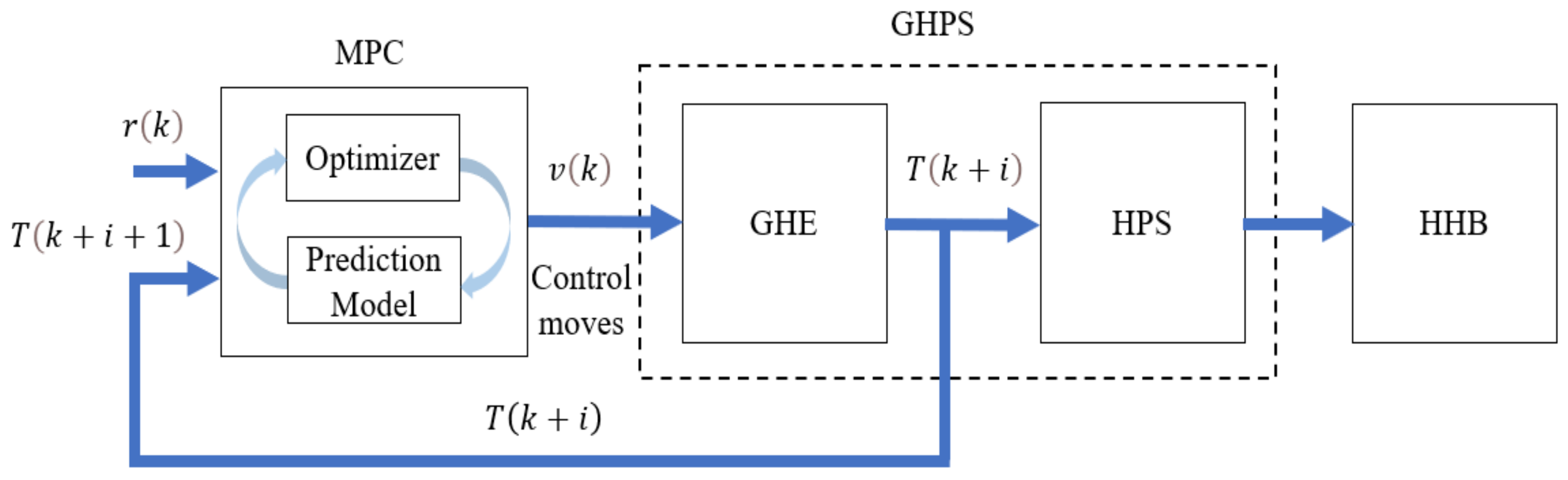
6. Model Predictive Control

Model predictive control (MPC) is a modern approach that relies on the plant model and its current state to solve open-loop optimization problems. MPC can predict future control actions to obtain the control model’s sequence, which can be used to enforce the predicted output signal to track the pre-defined reference signal while the error prediction is minimized. Typically, the first control action is only computed; it then moves forward with a new state and control prediction values while the pre-defined cost function is minimized. The MPC design is based on the system model’s discrete state space matrices (A, B, and C) and its critical parameters, the prediction horizon ( N P ) and control horizon ( N C ), used for tuning. These parameters, N P and N C , define the number of sample predictions and samples to control the system’s output, respectively. Furthermore, their values are chosen based on the following formula: 1 N C N P [49]. According to MPC’s advantages and robust performance, it may be appropriate to optimize the output temperature of the ground heat exchanger (GHE).

6.1. Prediction

The future system model output is predicted based on estimated control input vectors and future state variables through the prediction horizon N P . Thus, the future input control trajectory and future state variables can be expressed in Equations (25) and (26) as follows:
u k ,     u k + 1 ,   ,   u k + N c 1 ,
x k + 1 | k ,   x k + 2 | k ,   ,   x k + N p | k
where u k and x k are input control variable and state vector at time k , respectively. Implementing the input control and the state vector equations through iteration yields the predicted sequence of the output Y , which is shown below.
Y = F x k i +   U
where F , are matrices used in the prediction Equation (27)
F = C A C A 2 C A N P ;   = C B 0 0 C A B C B 0 C A 2 B C A B 0 C A N P 1 B C A N P 2 B C A N P N C B

6.2. Optimization

The control design’s objective is to enforce the GHE’s predicted output temperature T ^ k to track the pre-defined referenced signal r k i by determining the best control vector u (i.e., best water velocity) to minimize the prediction error (between the pre-defined referenced and predicted output temperature) through the prediction horizon N P . The pre-defined reference signal is defined below.
r k = r k + 1 r k + 2 r k + N p
By controlling the water velocity v k (input control variable), the future output temperature trajectory T ^   k + 1 can be predicted. while the cost function is minimized. The cost function equation J k is:
J k = i = 1 N p Q · [ T ^ k + i | k r k + i | k 2 + i = 1 N C 1 R · Δ v k + i | k 2 + i = 1 N P Q 1 · v k + i | k 2    
subject to
T m i n   T ^ k + i | k T m a x v m i n v k + i | k v m a x Δ v m i n Δ v k + i | k Δ v m a x
where T ^ k + i | k and r k + i | k are the predicted output temperature and the predefined reference temperature at the time k + i , respectively, while v k + i | k and Δ v k + i | k are predicted manipulated control and predicted rate manipulated control changes at the time k + i , respectively. The Q 1 , Q 2 , and R are the weightings of error output, input, and a variable rate of control change, respectively. Based on the system dynamics prediction, the cost function J k is integrated along the prediction horizon NP. It is important to note that all these positive weighting coefficients ( Q 1 , Q 2 , R ) should be defined in appropriate tuning ranges to ensure that the MPC operates according to the constraints, and then the following control variable sequences are computed to minimize the cost function. At each time step, the state matrices are updated to solve the quadratic problem (QP) to enhance the control performance along with the length prediction. Figure 5 shows the schematic diagram of model predictive control of heat transfer in a vertical ground heat exchanger for a geothermal heat pump system.

7. Case Study of a Geothermal Heat Pump System at Oakland University

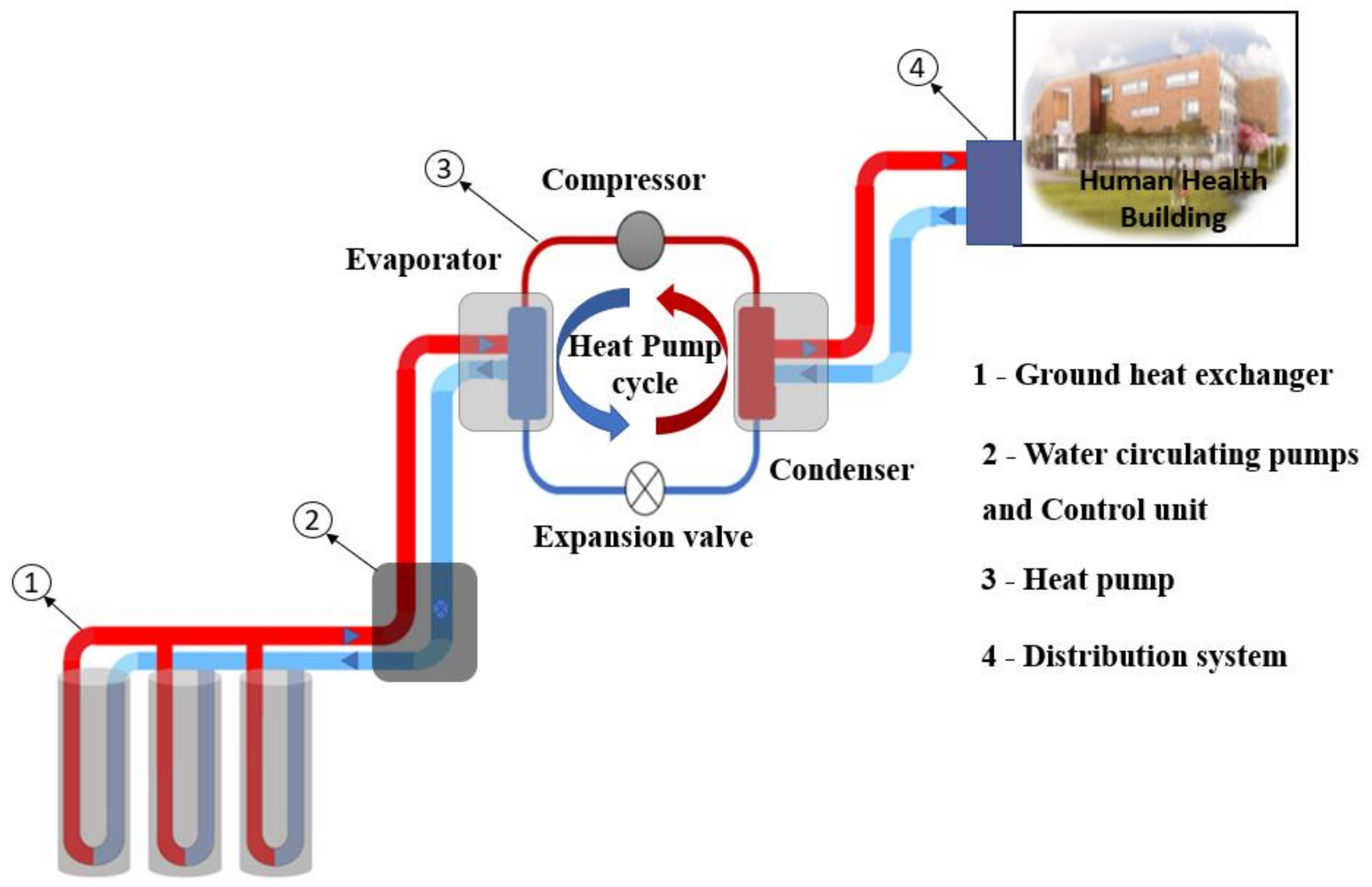
7.1. System Description

The 400-ton geothermal heat pump system (GHPS) was installed at Oakland University’s northwest campus in August 2012 to provide space heating and cooling for the Human Health Building (HHB). The HHB is a five-story building with a total area of 159 , 793   m 2 that requires a lot of heat and cooling energy; consequently, a vertical ground heat exchanger (GHE) with 256 vertical boreholes is appropriate. The GHPS typically consists of a vertical closed-loop ground heat exchanger (GHE), a heat pump, and a distribution unit system, as shown in Figure 6. The GHE consists of 256 vertical borehole arrays that were drilled to a depth of 98   m . A 7.62   m distance between two centered boreholes ensured that there was no interference between two U-tube GHE pipe’s legs. A high-density polyethylene (HDPE) pipe was inserted into each borehole as a single U-tube borehole configuration, with inner and outer diameters of 0.026   m and 0.032   m , respectively. These pipes were then connected to the heat pumps in parallel circuits. Backfilling the space between the pipe’s outer wall and the borehole wall with thermally enhanced bentonite grout with a high thermal conductivity created a strong connection between them. Table 2 demonstrates the geometric characteristics of the HDPE pipe. The ground loop pipes were filled with water (water-to-air, which is mostly used in the U.S.) for underground circulation that can promote heat exchange between the water inside the pipe and the surrounding ground by continually circulating the water. Forty-four heat pumps were connected parallel to two circulating 60 horsepower (HP) variable-frequency drive (VFD) water pumps that circulate the water inside the pipes at varying velocities as needed; when the first pump is active, the second is in standby mode [50]. When the heat arrived from the heat pump, the distribution unit circulated air through ducts to keep room temperatures consistent.
Since the GHPS started operating in August 2012, it has been supplying efficient heating and cooling to the HHB. Leidel [50] assessed the GHPS’s performance using its input and output temperature datasets between 2013 to 2015. The results showed that the temperature fluctuation was low, meaning that the underground heat exchanger loop pipes were appropriately sized and designed to provide enough heating and cooling for the entire building with excess capacity to supply more.
To keep the GHPS operating at optimum efficiency so that it can continue to provide the HHB with adequate temperatures in the winter and summer without wasting additional energy (used for heat and water circulating pumps), controlling water velocity is necessary. The MPC controller acts as an energy management system that minimizes energy consumption by optimizing the GHE’s output temperature. This is based on the MPC’s objective to control the water velocity in the U-tube pipe so that the GHE’s output temperature can be optimized by bringing the predicted output temperature as close to the pre-defined referenced output temperature as possible.

7.2. Physical Setup

The water velocity was not constant, but it was assumed to be 0.6 m / s   to determine the heat transfer convective coefficient h i . The convective heat transfer coefficients for both modes were calculated based on Equation (17), and they were 2105.70 and 2182.17 W / m 2 · for the heating and cooling modes, respectively.
Once the convective heat transfer coefficient was computed, it was substituted in Equation (18) to find the overall heat transfer coefficient U 0 . In the ground, the pipe had little room horizontally. This was defined in Equation (18) as R v .   The R-value was calculated as 0.1 per inch for the backfill soil material, which varies depending on composition, which in turn affects penetration depth. For example, it ranged from 5 to 15 inches, 40 to 75 inches, and 75 to 95 inches for the clay, sand, and good crushed rock, respectively [51]. In this study, the thermally enhanced bentonite grout with high thermal conductivity was used for the GHE at Oakland University. Thus, we assumed the pipe’s surrounding space to be 30 inches; therefore, R v = 0.0385   m 2 · / W . The GHE parameter values used in the simulation are presented in Table 3.
The overall heat transfer coefficient for both heating and cooling modes was 19.08 W / m 2 · . Despite differences in convective heat transfer coefficients for heating and cooling modes, the overall heat transfer coefficients were the same.

8. Results and Discussion

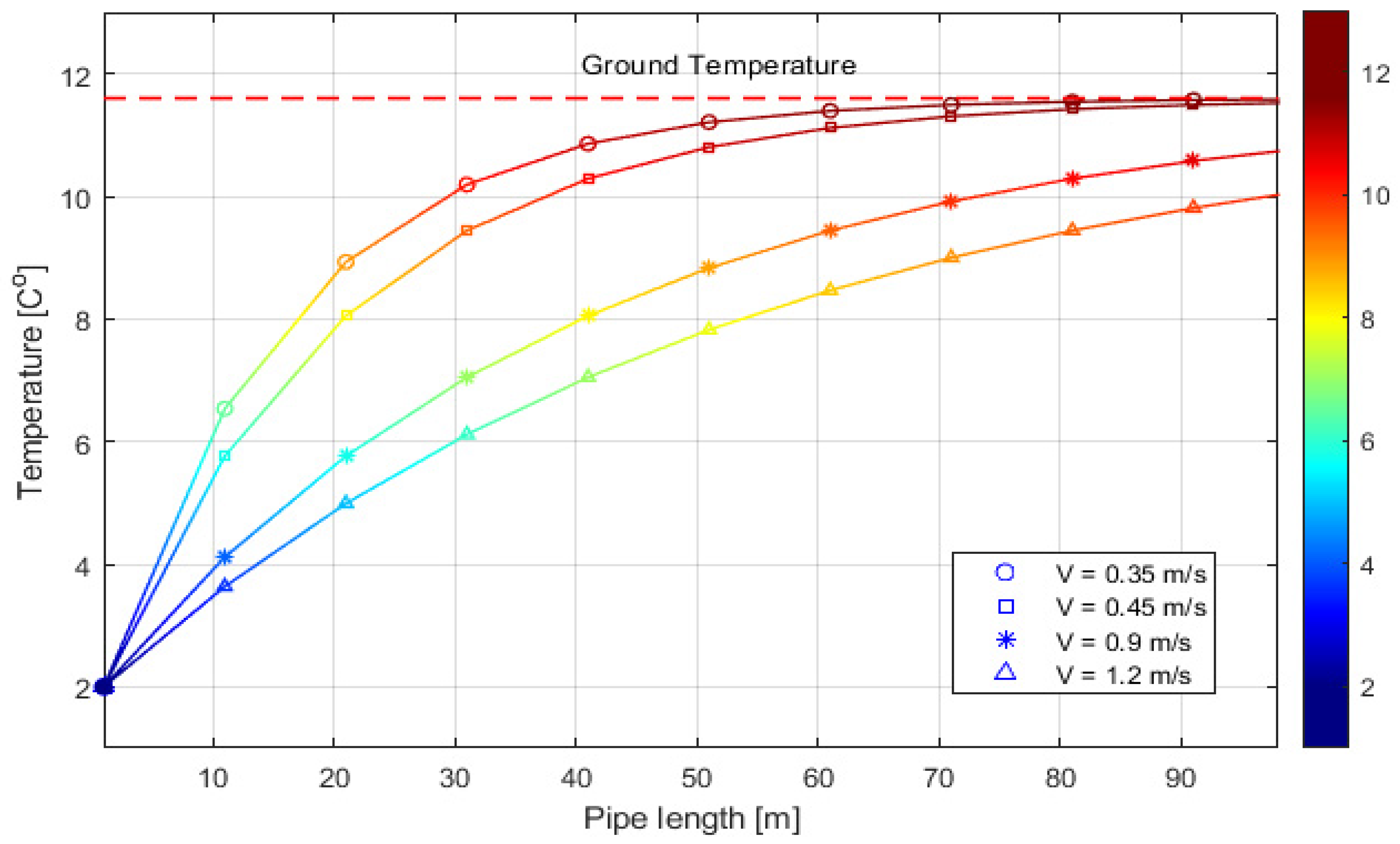
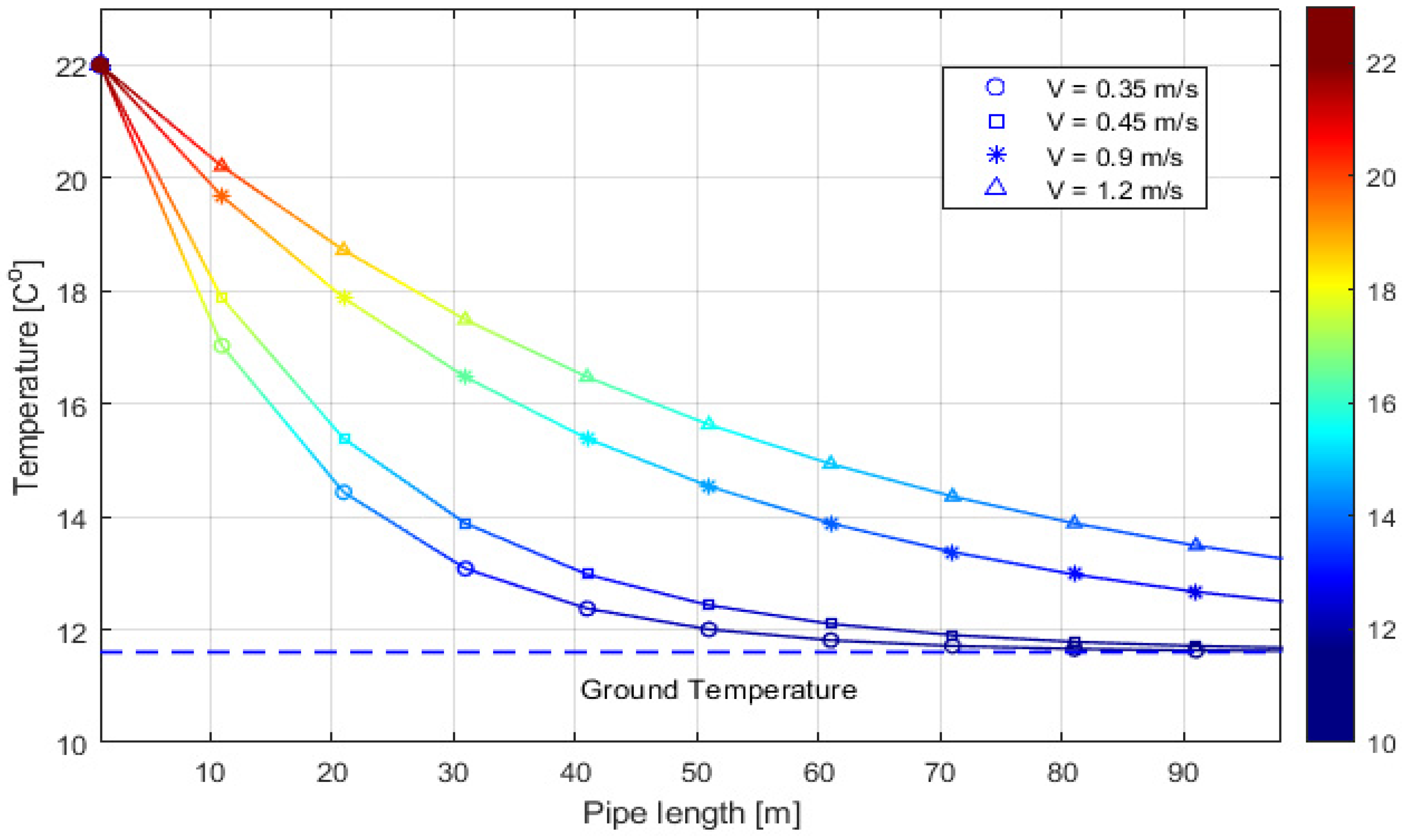
8.1. Implementation of the Heat Transfer Model in a Vertical Ground Heat Exchanger for Heating and Cooling Modes

The heat transfer behavior between the water temperature inside a vertical single U-tube pipe and its surrounding ground model for heating and cooling modes, and verification of the effect of the water velocity were demonstrated through simulations. To validate this, the proposed model was applied to evaluate the heat transfer behavior in GHE at Oakland University in both modes. The proposed heat transfer model (19) then was written in MATLAB’s script and implemented using an ordinary differential equation (ODE) solver with two initial conditions: T 0 = T i n , and T 0 = 0 . The model’s parameters defined in Table 2 and Table 3 were substituted into the same equation. The initial temperatures were set to T 0 =   2   ,   and 22   for winter and summer, respectively, referring to the temperature at x = 0 and flowing through the length of pipe   L . The ground temperature T g remained constant at 11.6     for both modes. Additionally, the working fluid (water) flowed at a uniform rate through the pipe at different velocities; however, the water velocity did affect the heat transfer performance and the exit temperature. Thus, four different water velocities, namely, 0.35 ,   0.45 , 0.9, and 1.2   m / s , respectively, were applied for the heating and cooling modes, thereby demonstrating how the water velocity affects the loop temperature. Consequently, the heat transfer model was implemented, and the water temperature behavior inside a vertical single U-tube pipe for heating and cooling modes was observed (depicted in Figure 7 and Figure 8). As expected, the GHE’s output temperature matched the ground temperature, which validated the proposed model.
The water temperature behavior inside a vertical single U-tube pipe at different velocities for the heating mode is depicted in Figure 7. The temperature T(x) increased exponentially during water flow inside the pipe from 2   until it reached the ground temperature of 11.6   at 90   m and 95   m from the pipe length when the water velocity was 0.35 and 0.45 m / s , respectively. The temperature then gradually remained stable throughout the pipe’s exit. In this case, the ground heat was transferred to the water inside the pipe. In Figure 7, we observed that the output temperature T x approached the ground temperature when the water velocity was between 0.35 and 0.45 m / s . However, it did not approach the ground temperature when the water velocity was increased to 0.9 and 1.2 m / s , despite reaching the pipe’s exit. Considerably more heat energy was wasted at these velocities.
Figure 8 demonstrates the water temperature behavior inside a vertical single U-tube pipe at different velocities for the cooling mode. According to Figure 8, the output temperature T x decreased exponentially along the pipe from 22   until it approached the ground temperature of 11.6   at 90.5   m and 95.5   m , when the water velocity was 0.35 and 0.45 m / s , respectively. That is, the water heat was transferred to the ground. However, the temperature T x did not reach the ground temperature when the water velocity was increased from 0.9 to 1.2 m / s , as shown in Figure 8.
According to this investigation of water velocity, it affected the temperature T x , which can impact the GHE’s thermal performance, as shown in Figure 7 and Figure 8. As the water velocity increased, there was less time for the water to reach the ground temperature, resulting in significant temperature differences ( Δ T ). This led to a larger margin of error because the water was flowing too fast to effectively reach the appropriate level. Thus, the temperature T x only reached that of the ground when the water velocity was lowered to the point where it had time to heat or cool.
The end of the pipe, 98   m , was chosen as a representative point in the comparison process. A comparison of the heat transfer in heating and cooling modes was performed, as depicted in Table 4.
When the water velocity was 0.33 and 0.43 m / s , Δ T was 0 for both heating and cooling modes, whereas when water velocity was 0.9 m / s , Δ T was 0.86 and 0.89 in heating and cooling, respectively. In addition, when the water velocity was 1.2 m / s , Δ T was 1.58 and 1.65 in heating and cooling, respectively. As a result, when the GHPS was set to its heating mode, the output temperature of GHE reached the ground temperature slightly faster than when it was set to its cooling mode. This indicates that heat transfer from the ground to the water inside the pipe was slightly faster than heat transfer from the water to the ground.
According to the findings, water velocities of 0.35 and 0.45 m / s were ideal for heat transfer. On the other hand, the velocities of 0.9 m / s and 1.2 m / s were too fast, not giving the water enough time to sufficiently reach the ground temperature. Pushing the water at high velocities provided no benefit, as it neither delivered an appropriate temperature for use nor saved energy; this has an impact on the heat pump’s operating efficiency. However, if the water velocity is kept low, the temperature T x will reach ground temperature before the pipe’s exit and will remain steady throughout the pipe, rendering the remaining piping loop useless. Therefore, the water velocity could be lowered sufficiently to reach the appropriate temperature without wasting any additional resources; for example, the circulation water pump needs more energy to increase its velocity. In addition, the heat pump needs to compensate for the heat that is not being delivered to the building.
To further demonstrate the performance of the proposed heat transfer model, it was used to simulate the GHE’s output temperature behavior for both U-tube De 25 mm (outer diameter of 25 mm ) and U-tube De 40 mm (outer diameter of 40 mm ) pipe diameters, as well as to identify the acceptable range of water velocities for these U-tube pipes. Note that the parameters used in this experimental study were the same as those used in the previous implementation of heat transfer behavior in the GHE at Oakland University, as shown in Table 2 and Table 3. Therefore, the acceptable ranges of water velocity were computed and are shown in Table 5.
In summary, the acceptable range of water velocity in a vertical single U-tube GHE pipe at Oakland University is between 0.35 and 0.45 m / s to ensure that the heat pump delivers the appropriate temperature to provide HHB with comfortable temperatures regardless of the season. According to our simulation results, the reasonable range of water velocity in vertical single U-tube De 25 mm , De 32 mm , and De 40 mm pipes are between 0.33 and 0.43 m / s , 0.35 to 0.45 m / s , and 0.38 to 0.48 m / s , respectively.

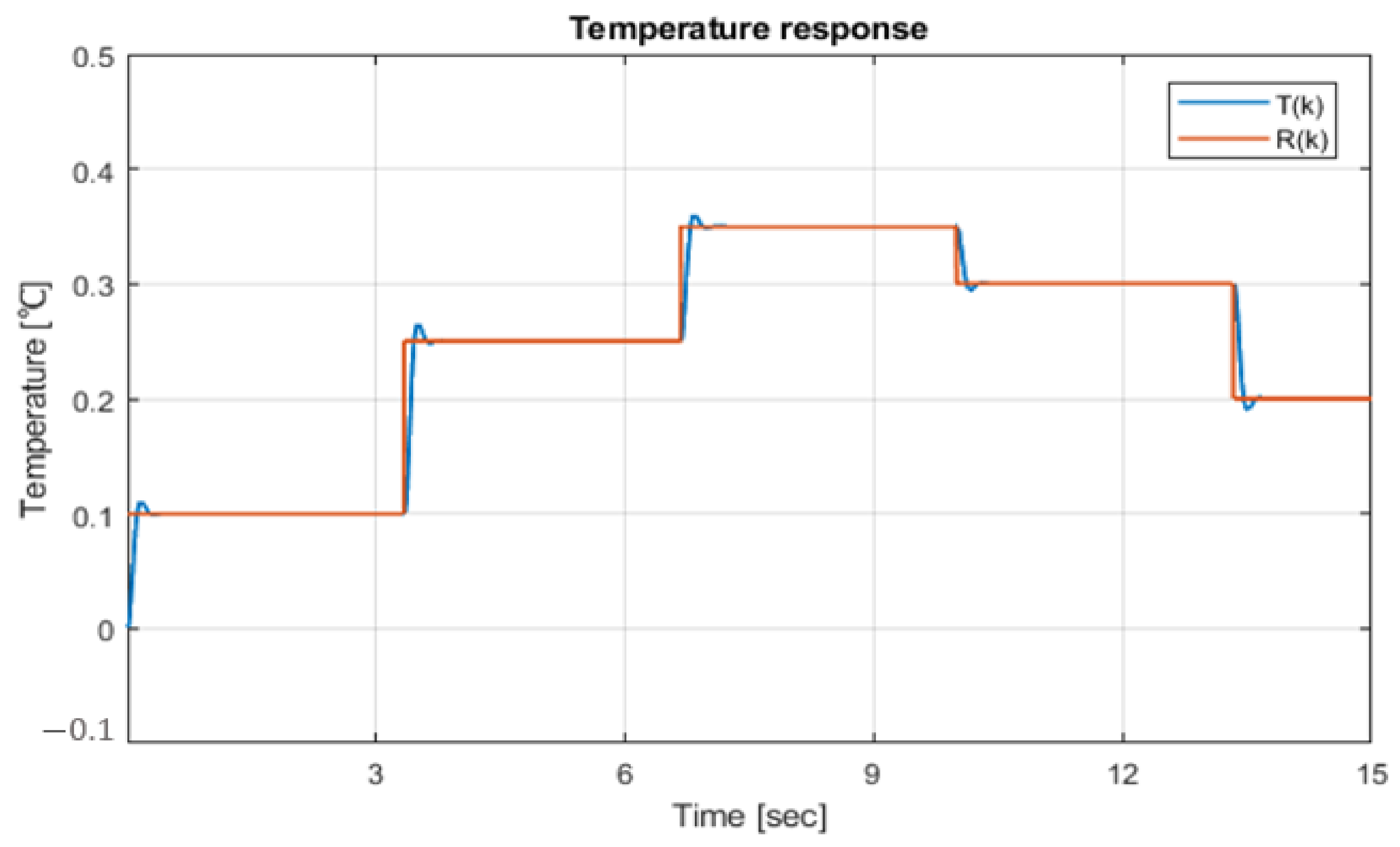
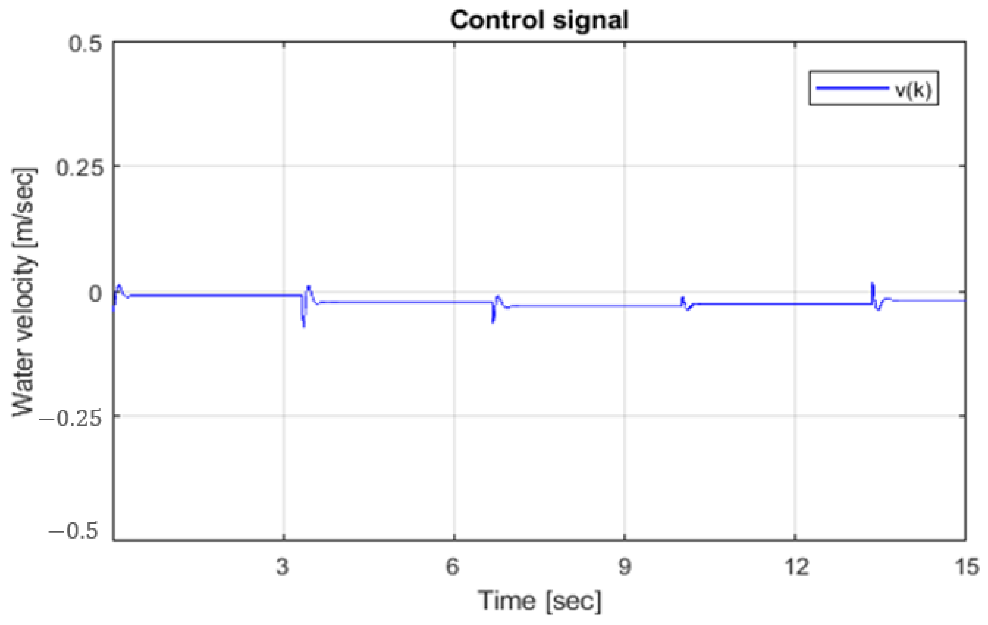
8.2. MPC Implementation and Simulation Results

According to the simulation results (see Figure 7 and Figure 8), circulating fluid in the U-tube pipe affects the GHE’s output temperatures and consumes energy, which will especially increase with higher velocities. To overcome this problem and optimize the GHE’s output temperature, which can improve energy consumption, we designed and implemented an MPC that can control the water velocity to optimize the GHE’s output temperature and keep it at the appropriate temperature. The MPC controller was designed to solve the quadratic problem (QP) subjected to input constraints 0.5 u k 0.5 along with the length prediction. The MPC’s objective is to control the water velocity so that it can enforce the GHE’s output temperature to track the pre-defined reference temperature as accurately as possible. This could be even more accurate because there are constraints on both the input and output signals. The MPC parameters used in this study were N P = 12 ,   N C = 2 , and T s = 0.01   s . All these parameters were accurately chosen and properly tuned to achieve strong performance and to reduce the error prediction between the predicted and pre-defined reference output temperature values over the prediction horizon. Consequently, the MPC model was implemented using the MATLAB script and the Simulink platform, and the GHE’s output temperature response and control signal were observed (depicted in Figure 9 and Figure 10).
.
According to Figure 9, the GHE’s output temperature tracked the reference temperature trajectory precisely, with a slight overshoot. This result reflects the optimal performance of the control design, and its performance was influenced by water velocity fluctuations.

9. Conclusions

The heat transfer model was proposed to evaluate the heat transfer behavior in the ground heat exchanger (GHE) between the water in the vertical U-tube pipe and its surrounding grounds for both the heating and cooling modes. The proposed model was applied to a case study, Oakland University’s GHPS, to evaluate its validation and enhance the GHE’s performance. Then, the model simulation results were performed using an ODE solver in MATLAB (R2021a) software. According to our findings, the output temperature only reached the ground for both modes when the water velocity was between 0.35 m / s and 0.45 m / s . This is, the heat transfer between two different heat sources required sufficient time to complete. The proposed model was validated when the GHE’s output temperature reached that of the ground. Furthermore, the influence of water velocity on the GHE’s output temperature was discussed. We identified that the optimum ranges of water velocity in vertical single U-tube pipes with diameters of De 25 mm , De 32 mm , and De 40 mm at a depth of 98   m was between 0.33 and 0.43 m / s , 0.35 to 0.45 m / s , and 0.38 to 0.48 m / s , respectively (see Table 5). Interestingly, the validation of the water temperature behavior in the ground heat exchanger will be the subject of future research.
The circulating fluid in the U-tube pipe affects the GHE’s output temperatures and consumes energy, which will increase as velocities increase. Therefore, we designed and implemented a model predictive control (MPC) controller to optimize the GHE’s output temperature by controlling the water velocity. The MPC was able to predict the future GHE’s output temperature, which resulted in well-tracking performance with the reference temperature trajectory, which was proven by the simulation result. This led to an improved reduction in the energy consumption used for heat and circulating water pumps and ensured that the heat pump delivered the appropriate temperature to provide the HHB with comfortable temperatures regardless of the season. We concluded that the designed linear MPC can control nonlinear heat transfer in a vertical ground heat exchanger system around the desired equilibrium point. In the future, we anticipate controlling this nonlinear system at several operational points, controlling each point separately, and switching between these controllers using the single controller block to control it more effectively along its trajectory.

Author Contributions

Conceptualization, K.S.; Investigation, C.J.K.; Methodology, K.S.; Software, K.S.; Supervision, M.Z.; Validation, C.J.K.; Writing—original draft, K.S.; Writing—review & editing, K.S. All authors have read and agreed to the published version of the manuscript.

Funding

This research received no external funding.

Institutional Review Board Statement

Not applicable.

Informed Consent Statement

Not applicable.

Data Availability Statement

Not applicable.

Conflicts of Interest

The authors declare no conflict of interest.

Nomenclature

List of abbreviations
BLSBilinear system
CO2Carbon dioxide
DBHEDeep borehole heat exchangers
DEPipe diameter
HDPEHigh-density polyethylene pipe
HPHorsepower
HHBHuman Health Building
HPSHeat pump system
HVACHeating and ventilation and air-conditioning
GHEGround heat exchanger
GHPSGeothermal heat pump system
MPCModel predictive control
ODEOrdinary differential equation
QPQuadratic problem
VFDVariable-frequency drive
List of symbols
A pipe’s cross-section area, m 2
A , B , C ,   and D matric of state–space
c p specific heat, kJ / kg ·
d i inner pipe diameter, m
d o outer pipe diameter, m
Esystem energy, W
F , matrices used in the prediction Equation (27)
h i convective heat transfer coefficient, W / m 2 ·
k discrete and time, s
t continuous time, s
k w water thermal conductivities, W / m ·
k p pipe thermal conductivity, W / m ·
L pipe length, m
m ˙ mass flow rate, kg / s
n heating/cooling exponent
N U d i Nusselt number
N C control horizons
N P prediction horizon
P r Prandtl number
P 0 pipe’s outside periphery, m
Qrate of heat transfer, W
Q ˙ x heat flow in at position x, W
Q ˙ x + Δ x heat flow out at x + Δ x , W
Q ˙ p the heat coming out of the water to the ground, W
Q 1 weighting of input error
Q 2 weighting of output error
r k reference signal at time k
R weightings of variable manipulated change
R c o n v fluid thermal resistance, m 2 · / W
R g ground thermal resistance, m 2 · / W
R w a l l pipe wall’s thermal resistance, m 2 · / W
R T H total thermal resistance, m 2 · / W
R v soil thermal resistance, m 2 · / W
R e d i Reynolds number
T s sample time, s
T temperature,
T k measured temperature at k ,
T ^ k predicted temperature at k ,
T x water temperature at position x ,
T i n t input temperatures,
T o u t output temperature,
T g ground temperature,
Δ T temperature difference,
U 0 overall heat transfer coefficient, W / m 2 ·
u k control signal at time k
v working fluid velocity, m / s
v m i n minimum constraint for v , m / s
v m a x maximum constrain for v , m / s
W s system work done, W
x k state vector at time k ,
y , Y measured and predicted outputs
List of Greek letters
µ dynamic viscosity, cp
ρ p pipe density, kg / m 3
ρ w water density, kg / m 3

References

  1. Omer, A.M. Ground-source heat pumps systems and applications. Renew. Sustain. Energy Rev. 2008, 12, 344–371. [Google Scholar] [CrossRef]
  2. Parsons, J. What is Geothermal Energy and How Can I Heat/Cool My House with It? 12 November 2020. Available online: https://www.climatemaster.com/homeowner/news/geothermal-energy/geothermal-energy/2020-12-11-what-is-geothermal-energy-and-how-can-i-heat-cool-my-house-with-it (accessed on 1 March 2022).
  3. Heat, G. Geothermal Energy Outlook Limited for Some Uses but Promising for; United States General Accounting Office: Washington, DC, USA, 1994.
  4. Miles, H. Heat Pump vs. Geothermal Systems: Which is Best? 15 February 2021. Available online: https://homeinspectioninsider.com/heat-pump-vs-geothermal-systems-which-is-best/ (accessed on 7 March 2022).
  5. Greensleeves Technologies Corp. CO2 Emissions and Geothermal. 18 October 2018. Available online: https://www.greensleevestech.com/co2-emissions-and-geothermal/ (accessed on 15 March 2022).
  6. Manitoba Geothermal Energy Alliance. Available online: https://www.mgea.ca/lead-project/the-forks/ (accessed on 1 April 2022).
  7. Kavanaugh, S.P. A design method for hybrid ground-source heat pumps. ASHRAE Trans. 1998, 104, 691. [Google Scholar]
  8. Zhou, H.; Lv, J.; Li, T. Applicability of the pipe structure and flow velocity of vertical ground heat exchanger for ground source heat pump. Energy Build. 2016, 117, 109–119. [Google Scholar] [CrossRef]
  9. Akpinar, E.K.; Hepbasli, A. A comparative study on exergetic assessment of two ground-source (geothermal) heat pump systems for residential applications. Build. Environ. 2007, 42, 2004–2013. [Google Scholar] [CrossRef]
  10. Akrouch, G.A.; Sánchez, M.; Briaud, J.-L. An experimental, analytical and numerical study on the thermal efficiency of energy piles in unsaturated soils. Comput. Geotech. 2016, 71, 207–220. [Google Scholar] [CrossRef]
  11. Wang, Z.; Wang, F.; Ma, Z.; Wang, X.; Wu, X. Research of heat and moisture transfer influence on the characteristics of the ground heat pump exchangers in unsaturated soil. Energy Build. 2016, 130, 140–149. [Google Scholar] [CrossRef]
  12. Tang, F.; Nowamooz, H. Factors influencing the performance of shallow Borehole Heat Exchanger. Energy Convers. Manag. 2018, 181, 571–583. [Google Scholar] [CrossRef]
  13. Choi, W.; Ooka, R. Effect of natural convection on thermal response test conducted in saturated porous formation: Comparison of gravel-backfilled and cement-grouted borehole heat exchangers. Renew. Energy 2016, 96, 891–903. [Google Scholar] [CrossRef]
  14. Lee, C.; Lee, K.; Choi, H.; Choi, H.-P. Characteristics of thermally-enhanced bentonite grouts for geothermal heat exchanger in South Korea. Sci. China Technol. Sci. 2010, 53, 123–128. [Google Scholar] [CrossRef]
  15. Lee, C.; Park, S.; Lee, D.; Lee, I.-M.; Choi, H. Viscosity and salinity effect on thermal performance of bentonite-based grouts for ground heat exchanger. Appl. Clay Sci. 2014, 101, 455–460. [Google Scholar] [CrossRef]
  16. Shadley, J.; Den Braven, K. Thermal Conductivity of Backfill Materials for Inground Heat Exchangers; American Society of Mechanical Engineers: New York, NY, USA, 1995. [Google Scholar]
  17. Book, J.D. Heat Transfer, 5th ed.; Japanese Society of Mechanical Engineers: Tokyo, Japan, 2009. [Google Scholar]
  18. VDI. Thermal Use of the Underground: Ground Source Heat Pump Systems; Richtlinien VDI 4640, Blatt 2; Verein Deutscher Ingenieure Düsseldorf: Düsseldorf, Germany, 2001. [Google Scholar]
  19. Jobmann, M.; Buntebarth, G. Influence of graphite and quartz addition on the thermos-physical properties of bentonite for sealing heat-generating radioactive waste. Appl. Clay Sci. 2009, 44, 206–210. [Google Scholar] [CrossRef]
  20. Dehkordi, S.E.; Schincariol, R.A. Effect of thermal-hydrogeological and borehole heat exchanger properties on performance and impact of vertical closed-loop geothermal heat pump systems. Appl. Hydrogeol. 2013, 22, 189–203. [Google Scholar] [CrossRef]
  21. Alberti, L.; Angelotti, A.; Antelmi, M.; La Licata, I. A numerical study on the impact of grouting material on borehole heat exchangers performance in aquifers. Energies 2017, 10, 703. [Google Scholar] [CrossRef] [Green Version]
  22. Jahanbin, A. Thermal performance of the vertical ground heat exchanger with a novel elliptical single U-tube. Geothermics 2020, 86, 101804. [Google Scholar] [CrossRef]
  23. Zhang, W.; Yang, H.; Lu, L.; Fang, Z. Investigation on influential factors of engineering design of geothermal heat exchangers. Appl. Therm. Eng. 2015, 84, 310–319. [Google Scholar] [CrossRef]
  24. Darkwa, J.; Su, W.; Chow, D. Heat dissipation effect on a borehole heat exchanger coupled with a heat pump. Appl. Therm. Eng. 2013, 60, 234–241. [Google Scholar] [CrossRef]
  25. High-Density Polyethylene (HDPE). 2022. Available online: https://polymerdatabase.com/Commercial%20Polymers/HDPE.html (accessed on 5 March 2022).
  26. Bassiouny, R.; Ali, M.R.; Hassan, M.K. An idea to enhance the thermal performance of HDPE pipes used for ground-source applications. Appl. Therm. Eng. 2016, 109, 15–21. [Google Scholar] [CrossRef]
  27. Raymond, J.; Frenette, M.; Leger, A.; Magni, E.; Therrien, R. Numerical modeling of thermally enhanced pipe performances in vertical ground heat exchangers. ASHRAE Trans. 2011, 117, 899. [Google Scholar]
  28. Bouhacina, B.; Saim, R.; Oztop, H.F. Numerical investigation of a novel tube design for the geothermal borehole heat exchanger. Appl. Therm. Eng. 2015, 79, 153–162. [Google Scholar] [CrossRef]
  29. Song, X.; Wen, Z.; SI, J. CFD numerical simulation of a U-tube ground heat exchanger used in ground source heat pumps. Chin. J. Eng. 2007, 29, 329–333. [Google Scholar]
  30. Zeng, H.; Diao, N.; Fang, Z. Heat transfer analysis of boreholes in vertical ground heat exchangers. Int. J. Heat Mass Transf. 2003, 46, 4467–4481. [Google Scholar] [CrossRef]
  31. Zarrella, A.; Emmi, G.; De Carli, M. A simulation-based analysis of variable flow pumping in ground source heat pump systems with different types of borehole heat exchangers: A case study. Energy Convers. Manag. 2017, 131, 135–150. [Google Scholar] [CrossRef]
  32. Gultekin, A.; Aydin, M.; Sisman, A. Thermal performance analysis of multiple borehole heat exchangers. Energy Convers. Manag. 2016, 122, 544–551. [Google Scholar] [CrossRef]
  33. Zheng, Z.; Wang, W.; Ji, C. A study on the thermal performance of vertical U-tube ground heat exchangers. Energy Procedia 2011, 12, 906–914. [Google Scholar] [CrossRef] [Green Version]
  34. Jun, L.; Xu, Z.; Jun, G.; Jie, Y. Evaluation of heat exchange rate of GHE in geothermal heat pump systems. Renew. Energy 2009, 34, 2898–2904. [Google Scholar] [CrossRef]
  35. Qi, D.; Pu, L.; Sun, F.; Li, Y. Numerical investigation on thermal performance of ground heat exchangers using phase change materials as grout for ground source heat pump system. Appl. Therm. Eng. 2016, 106, 1023–1032. [Google Scholar] [CrossRef]
  36. Cui, Y.; Zhu, J. 3D transient heat transfer numerical analysis of multiple energy piles. Energy Build. 2017, 134, 129–142. [Google Scholar] [CrossRef]
  37. Bauer, D.; Heidemann, W.; Müller-Steinhagen, H.; Diersch, H.-J.G. Thermal resistance and capacity models for borehole heat exchangers. Int. J. Energy Res. 2011, 35, 312–320. [Google Scholar] [CrossRef]
  38. Dada, M.; Benchatti, A. Assessment of Heat Recovery and Recovery Efficiency of a Seasonal Thermal Energy Storage System in a Moist Porous Medium. Int. J. Heat Technol. 2016, 34, 701–708. [Google Scholar] [CrossRef] [Green Version]
  39. Neuberger, P.; Adamovský, R.; Šeďová, M. Temperatures and heat flows in a soil enclosing a slinky horizontal heat exchanger. Energies 2014, 7, 972–987. [Google Scholar] [CrossRef] [Green Version]
  40. Asadi, A. A guideline towards easing the decision-making process in selecting an effective nanofluid as a heat transfer fluid. Energy Convers. Manag. 2018, 175, 1–10. [Google Scholar] [CrossRef]
  41. Diglio, G.; Roselli, C.; Sasso, M.; Channabasappa, U.J. Borehole heat exchanger with nanofluids as heat carrier. Geothermics 2018, 72, 112–123. [Google Scholar] [CrossRef]
  42. Narei, H.; Ghasempour, R.; Noorollahi, Y. The effect of employing nanofluid on reducing the bore length of a vertical ground-source heat pump. Energy Convers. Manag. 2016, 123, 581–591. [Google Scholar] [CrossRef]
  43. Li, Y.; Mao, J.; Geng, S.; Han, X.; Zhang, H. Evaluation of thermal short-circuiting and influence on thermal response test for borehole heat exchanger. Geothermics 2013, 50, 136–147. [Google Scholar] [CrossRef]
  44. Wang, Z.; Wang, F.; Liu, J.; Ma, Z.; Han, E.; Song, M. Field test and numerical investigation on the heat transfer characteristics and optimal design of the heat exchangers of a deep borehole ground source heat pump system. Energy Convers. Manag. 2017, 153, 603–615. [Google Scholar] [CrossRef]
  45. You, S.; Cheng, X.; Guo, H.; Yao, Z. In-situ experimental study of heat exchange capacity of CFG pile geothermal exchangers. Energy Build. 2014, 79, 23–31. [Google Scholar] [CrossRef]
  46. Casasso, A.; Sethi, R. Sensitivity Analysis on the Performance of a Ground Source Heat Pump Equipped with a Double U-pipe Borehole Heat Exchanger. Energy Procedia 2014, 59, 301–308. [Google Scholar] [CrossRef] [Green Version]
  47. Landegren, G.F. Newton’s law of cooling. Am. J. Phys. 1957, 25, 9. [Google Scholar] [CrossRef]
  48. Dittus, F.W. Heat transfer in automobile radiators of the tubler type. Univ. Calif. Pubs. Eng. 1930, 2, 443. [Google Scholar]
  49. Wang, L. Model Predictive Control System Design and Implementation Using MATLAB®; Springer Science & Business Media: Berlin, Germany, 2009. [Google Scholar]
  50. Leidel, J. Human Health Science Building Geothermal Heat Pump Systems; Oakland University: Rochester, MI, USA, 2014. [Google Scholar]
  51. Soil R-Value. 2022. Available online: http://geotechnicalinfo.com/r_value.html (accessed on 20 March 2022).
Figure 1. GHE’s thermal performance factors.
Energies 15 05300 g001
Figure 2. Schematic diagram of heat transfer profile for the GHE’s behaviors in (a) heating mode and (b) cooling mode. T (temperature), T i n t (input temperature), T o u t (output temperature), T(x) (water temperature at position x), T g (ground temperature), ∆T (temperature difference), and L (pipe length).
Energies 15 05300 g002
Figure 3. The rate of heat transfer through the pipe’s surface to the ground.
Energies 15 05300 g003
Figure 4. Schematic diagram of a vertical single U-tube ground heat exchanger (GHE) configuration, where d i is pipe inner diameter, d o is pipe outer diameter, T is temperature, R c o n v is fluid thermal resistance, R w a l l is pipe wall’s thermal resistance, R g is ground thermal resistance, and T g is ground temperature.
Energies 15 05300 g004
Figure 5. Schematic diagram of closed-loop controlling heat transfer in a ground heat exchanger for a geothermal heat pump system with MPC, where MPC is model predictive control, GHE is ground heat exchanger, HPS is heat pump system, GHPS is geothermal heat pump system, HHB is Human Health Building at Oakland University, r k is reference signal, T k is temperature, and v k is water velocity.
Energies 15 05300 g005
Figure 6. Schematic diagram of Oakland University’s GHPS.
Energies 15 05300 g006
Figure 7. The water temperature behavior in a vertical single U-tube for heating mode (in the winter) at different water velocities (0.35, 0.45, 0.9, and 1.2 m / s ).
Energies 15 05300 g007
Figure 8. The water temperature behavior in a vertical single U-tube for cooling mode (in the summer) at different water velocities (0.35, 0.45, 0.9, and 1.2 m / s ).
Energies 15 05300 g008
Figure 9. GHE output temperature T k tracing the reference temperature trajectory R K by MPC.
Energies 15 05300 g009
Figure 10. MPC control signal; water velocity v k ( m / s ) .
Energies 15 05300 g010
Table 1. Properties of some soil materials.
Parameter Density (kg/m3)Specific Heat Capacity (J/(kg K))Thermal Conductivity (W/m·K)
Sand150017101.13
Clay170018001.2
Sandy-silt184712001.3
Sandy-clay196012002.1
Table 2. HDPE piping system geometric characteristics.
SymbolValue Description
k p 0.5   W / m   · Thermal conductivity
d i 0.026   m Inner diameter
d o 0.032   m Outer diameter
ρ p 959.98   kg / m 3 Density
L 98   m length
Table 3. Parameters of the ground heat exchanger (GHE).
Symbol ValueUnitDescription
WinterSummer
µ1.7260.974 cp Dynamic viscosity
ρ999.94997.96 kg / m 3 Water density
C p 4.224.15 kJ / kg   · Specific heat
k w 0.598 0.598 W / m   · Water thermal conductivity
v 0.35–0.450.35–0.45 m / s Water velocity
n 0.40.3-Heating/cooling exponent
h i 2105.70 2182.17 W / m 2 · Convective heat transfer coefficients
U 0 19.0819.08 W / m 2 · Overall heat transfer coefficient
R v 0.03850.0385 m 2 · / W Soil thermal resistance
T i n 2 22   Input temperature
T g 11.6 11.6   Ground temperature
Table 4. Comparison of model heat transfer performances in heating and cooling modes.
Water Velocity
(m/s)
 Heating   Mode Δ T = T g T x ,
(the Pipe’s End, 98 m)
 Cooling   Mode Δ T = T x T g ,
(the Pipe’s End, 98 m)
0.3500
0.4500
0.90.860.89
1.21.581.65
Table 5. Acceptable ranges of water velocity in varying vertical single U-tube diameters.
U-Tube Pipe DiametersRange of Water Velocity
U-tube De 25 mm 0.33 0.43   m / s
U-tube De 32 mm 0.35 0.45   m / s
U-tube De 40 mm 0.38 0.48   m / s
Publisher’s Note: MDPI stays neutral with regard to jurisdictional claims in published maps and institutional affiliations.

