Modeling, Optimization, and Analysis of a Virtual Power Plant Demand Response Mechanism for the Internal Electricity Market Considering the Uncertainty of Renewable Energy Sources

Abstract

The penetration of renewable energy sources (RESs) in the electrical power system has increased significantly over the past years due to increasing global concern about climate change. However, integrating RESs into the power market is highly problematic. The output of RESs such as wind turbines (WTs) and photovoltaics (PVs) is highly uncertain. Their correlation with load demand is not always guaranteed, which compromises system reliability. Distributed energy resources (DERs), especially demand response (DR) programs and energy storage systems (ESSs), are possible options to overcome these operational challenges under the virtual power plant (VPP) setting. This study investigates the impact of using a DR program and battery energy storage system (BESS) on the VPP’s internal electricity market, and also cost-minimization analysis from a utility viewpoint. Three different constrained optimal power flow (OPF) problems are solved such as base case, DR case, and BESS case to determine total incurred costs, locational marginal prices (LMPs), and generator commitments. A scenario tree approach is used to model the uncertainties associated with WTs, PVs, and load demand. The proposed model is investigated on a 14-bus distribution system. The simulation results obtained demonstrate a favorable impact of DR and a BESS on renewable operational challenges.

1. Introduction

The penetration of renewable energy sources (RESs) in the energy market has shown significant growth over the past years. Typically, this is due to the following factors: global concern about climate change, carbonization of the environment, pollution, and clean energy requirements. Many countries, including China, America, Germany, Australia, UK, and Europe, have started incentive programs to encourage investment in renewable power plants, enabling these plants to participate in the power market or offer reserve capacity services to power systems [1,2,3,4,5].

However, integrating RESs such as (WTs and PVs) into the power market has been recognized as one of the potential problems facing utility grids. PV and WT inconsistent generation leads to commercial and technical problems such as voltage violation, power market commitment, unit commitment, and spinning reserves, all of which contribute to operational instability of the power system [6,7,8,9,10,11]. Therefore, to address these challenges, system operators must consider developing innovative approaches and models to manage the inherent unpredictability that comes with WT and PV technologies.

The integration of DR with a BESS is one possible option to mitigate the unpredictability of wind and solar generation. Therefore, implementing a DR program and a BESS model with the aim of minimizing renewable operational challenges will have an impact on the utility’s total operating costs, as it will alter the commitment of the generators. Moreover, it would have an effect on the energy prices due to the fluctuation in the costs. The energy storage system is another possibility that offers financial advantages and minimizes the impact of renewable generator uncertainty. The BESS stores energy during off-peak hours and then releases it during peak hours or when it is most needed. Therefore, this study aims to provide a stochastic approach, evaluating the impact of a DR program with a BESS on utility cost minimization. The impact of DR on locational marginal pricing is also examined, taking into account uncertainties related to wind speed, solar irradiance, and load demand. Three different constrained OPF problems are formulated (i.e., base case, DR case, and BESS case). The results of three different cases, each reflecting one of the three challenges, are compared and analyzed to demonstrate the impact of the DR program and a BESS on overall utility cost minimization.

1.1. Literature Review and Research Gap

In recent years, some of the most appropriate and closely related research on the key elements of energy utilization proposed in the literature review under the VPP environment are as follows. The authors of [12] concentrated on the optimal scheduling of a market-based VPP, operating in the day-ahead and real-time market with the aim of maximizing its own profit while mitigating purchasing costs. The authors of [13] presented a novel market bidding mechanism that enables a VPP to regulate the balancing energy market as either a passive or an active regulator. As a result, a VPP can increase its profitability by utilizing this market model. The authors of [14] evaluated a VPP energy trading model that aggregates RES, ESS, and electrical loads to maximize social welfare. The authors of [15] investigated hybrid AC-DC microgrids to maximize social welfare. However, the importance of ESS for renewable energy sources is disregarded. The authors of [16] investigated a VPP as a price maker to alleviate the RTM penalty by modeling the unpredictable resources with interval interpretation. In [17], the authors investigated a multi-objective-based VPP bidding strategy that considers (WT and PV) systems engaging in spinning and the energy markets to optimize profit while reducing emissions. In [18], the authors proposed a cost-minimization mechanism for a VPP engaging in demand-side management schemes. The authors of [19] have analyzed VPP interactive characteristics in the distribution systems providing energy flexibility support services in the distribution system without considering the uncertainty of RESs. The authors of [20] have proposed a technique for multi-stage market transactions that characterized VPP participation and evaluated the significance of VPP collaboration, but they did not account for DGs uncertainties. The estimated generation of a VPP may deviate from the actual generation due to uncertainties. Consequently, the VPP’s actual profit falls short of its target profit. Therefore, it is necessary to consider DG uncertainties. In [21], The authors developed a market-based model to evaluate the dispatch capability of (WT, PV, and ESS) with the aim of maximizing the social welfare of the participating members. This paper attempts to fill a gap in the literature which is to evaluate systematically the impact of the DR program with a BESS on the internal electricity market of VPP, locational marginal prices, and also on renewable generators’ stochastic challenges (i.e., WTs and PVs). The uncertainties related to wind speed, solar irradiance, and load demand are taken into consideration.

Table 1. Comparison of the proposed method with existing literature.

References	RES Management	DR Model	BESS Model	Uncertainty Modeling	Power Market
[12]	No	No	Yes	No	Yes
[13]	Yes	No	Yes	Yes	Yes
[14]	Yes	No	Yes	No	Yes
[15]	Yes	No	No	Yes	Yes
[16]	Yes	No	Yes	Yes	Yes
[17]	Yes	No	No	Yes	No
[18]	Yes	Yes	No	No	No
[19]	Yes	Yes	Yes	No	No
[20]	Yes	No	Yes	No	Yes
[21]	Yes	No	Yes	Yes	No
This paper	Yes	Yes	Yes	Yes	Yes

shows a comparison of the proposed model with existing literature.

1.2. Contributions and Study Layout

The following are the key contributions of this work in regards to the literature reviewed.

• The proposed strategy is designed and developed to visualize the trading of electricity within the VPP environment. This strategy encourages consumers to minimize their load at peak hours, while energy storage systems and distributed generators are also used to their full possible capacity, contributing to balancing the system’s total net load.
• The constrained OPF problem is formulated as an optimization problem, and the relevant solutions are obtained for each of the three cases in terms of cost minimization. Load curtailment of the Internal consumers has a favorable effect on the VPP’s aim of minimizing costs.
• The results obtained from the three test cases are comprehensively compared and analyzed and it was found that a DR program application has a significant impact on the VPP’s internal electricity market cost minimization as compared to the base case model and BESS model.

The remainder of the paper is structured as follows: Section 2 explains the aim and approach of the study. Section 3 presents uncertainty modeling related to wind speed, solar irradiance, and load demand. The mathematical formulations of the base case, DR program, and BESS model are presented in Section 4. The VPP electricity market structure is described in Section 5. The case study, simulation results, and discussion are presented in Section 6. A locational marginal costs comparison is presented in Section 7, and finally, some meaningful conclusions are drawn in Section 8.

2. Aim and Approach

This study aims to evaluate the benefits of implementing a DR program and running a BESS to minimize the operational challenges of RESs on distribution networks. The proposed approach is compared to a conventional OPF solution. A constrained OPF is used as an optimization problem for three different cases including a base case, DR program, and a BESS, subject to equality and inequality constraints of the system. Furthermore, the impact of the DR program and a BESS on LMPs are also examined. A scenario-based method is applied to model the uncertainties associated with wind speed, solar irradiation, and electrical load demand. The method analyzes the impact of the DR program on WTs, PV power generation, and a BESS active power delivery capacity to load over the planning horizon to minimize costs from a utility perspective.

3. Uncertainty Modeling

The scenario tree approach is used to model the uncertainties associated with wind speed, solar irradiation, and load demand, where a scenario is described as a possible realization of an uncertain parameter. The probability density function (PDF) is used for each wind speed, solar irradiation, and load demand to generate 24 scenarios.

3.1. Wind Speed Modeling

The wind speed variation in a specific area is modeled using the Weibull PDF [22,23,24]. The PDF function that correlates the wind speed and the WT module output power is expressed by [1].

$$PDF(\nu )=\left(\frac{k}{c}\right){\left(\frac{\nu }{c}\right)}^{k-1}\exp \left[-{\left(\frac{\nu }{c}\right)}^k\right]$$

(1)

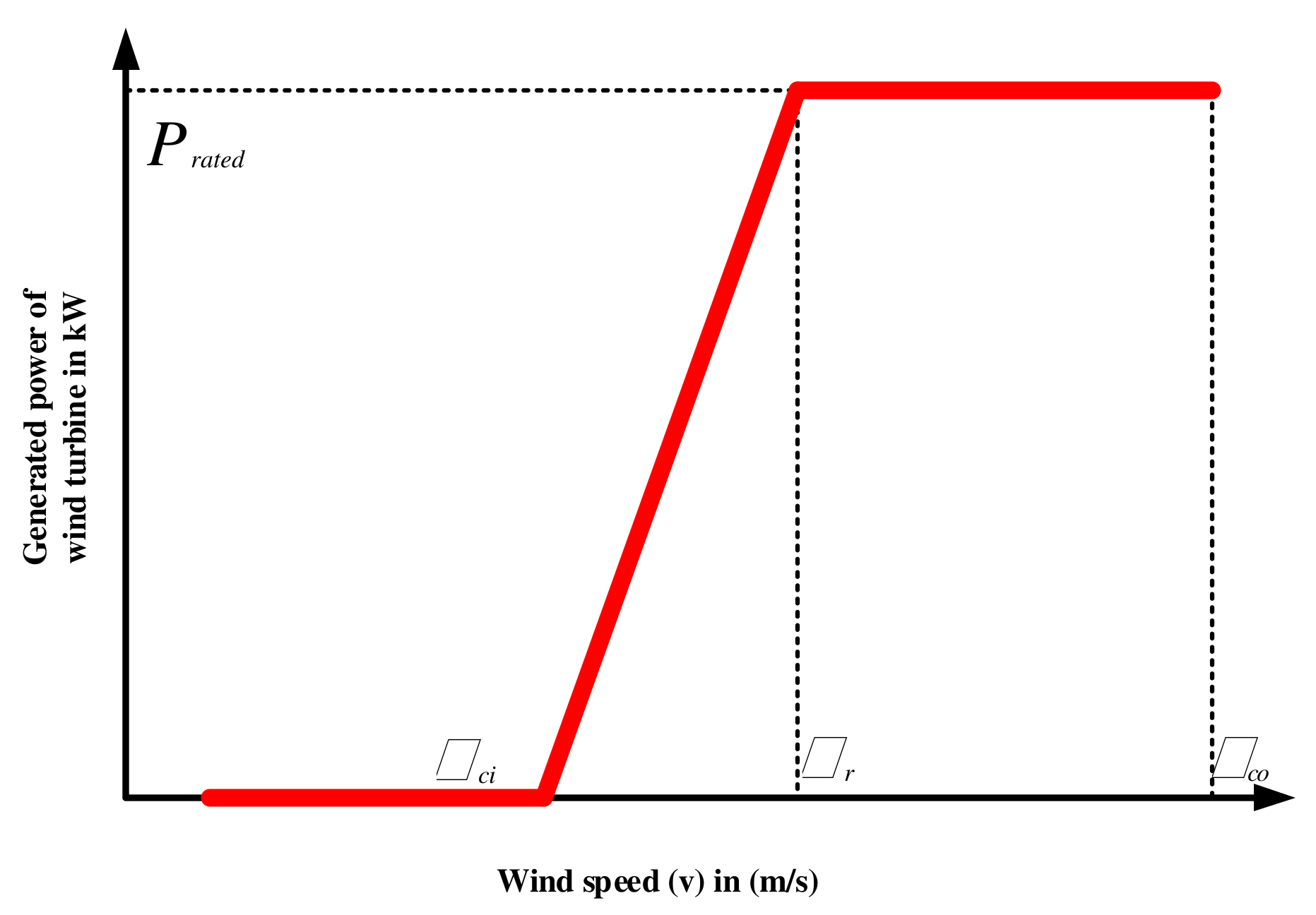
where ν, c, and k represent the wind speed, Weibull PDF scale index, and shape index. Therefore, the WT module output power can be examined by employing its power curve.

$${{\displaystyle P}}_{wt}(\nu )=\left\{\begin{array}{ll}0,& 0\le \nu \le {{\displaystyle \nu }}_{ci}\\ {{\displaystyle P}}_{rated,}\times \frac{\nu -{{\displaystyle \nu }}_{ci}}{{{\displaystyle \nu }}_r-{{\displaystyle \nu }}_{ci}},& {{\displaystyle \nu }}_{ci}\le \nu \le {{\displaystyle \nu }}_r\\ {{\displaystyle P}}_{rated,}& {{\displaystyle \nu }}_r\le \nu \le {{\displaystyle \nu }}_{co}\\ 0,& {{\displaystyle \nu }}_{co}\le \nu \end{array}\right.$$

(2)

where P_wt and P_rated represent the WT output power and the rated power. ${\nu }_{ci}$ and ${\nu }_{co}$ represent the cut-in and cut-out speed. The rated speed of WT is represented by ${\nu }_r$ [15,22,25]. The wind speed power curve of WT is shown in Figure 1.

Thus, the output power of the WT module at bus i and scenario w can be expressed as follows:

$$0\le {{\displaystyle P}}_{i,w}^{wt}\le {{\displaystyle \gamma }}_{i,w}^{wt}\times {{\displaystyle P}}_{i.rated}^{wt}$$

(3)

where ${{\displaystyle \gamma }}_{i,w}^{wt}$ is the WT power generation percentage.

3.2. Modeling of Solar Irradiance

The beta PDF is employed to model solar irradiance as presented by Equation (4).

$$PDF(S)=\left\{\begin{array}{ll}\frac{\Gamma (\alpha +\beta )}{\Gamma (\alpha )+\Gamma (\beta )}\times {{\displaystyle s}}^{\alpha -1}\times {{\displaystyle (1-s)}}^{\beta -1},& 0\le s\le 1,0\le \alpha ,\beta \\ 0& \hspace{1em}\hspace{1em}\hspace{1em}else\end{array}\right\}$$

(4)

The solar irradiance in kilowatt per meter square is represented by S. The beta PDF parameters (i.e., α and β) can be determined as follows:

$$\beta =(1-\mu )\times \left(\frac{\mu \times (1-\mu )}{{{\displaystyle \sigma }}^2}-1\right)$$

(5)

$$\alpha =\frac{\mu \times \beta }{1-\mu }$$

(6)

where µ and σ denote the mean value and the standard deviation. Solar irradiation and ambient temperature are the key parameters in determining the PV module output power, expressed by using Equations (5) and (6)

$${{\displaystyle P}}_{PV}={{\displaystyle P}}_{STC}\left\{\frac{G}{100}\left[1+\delta \left({{\displaystyle T}}_{cell}-25\right)\right]\right\}$$

(7)

$${{\displaystyle T}}_{cell}={{\displaystyle T}}_{amb}+\left(\frac{NOCT-20}{800}\right)G$$

(8)

where P_STC and P_PV denote the power in (MW) under standard test conditions and the PV module output power in kilowatts, respectively. The power–temperature coefficient in (%/°C) is denoted by δ. T_amb, T_cell, and NOCT represent the ambient temperature in °C, the cell temperature in °C, and the nominal operating cell temperature conditions in °C. G represents solar irradiance in watt per meter square [26,27,28,29].

3.3. Load Demand Uncertainty Modeling

The normal PDF function is used to model each bus’s load demand. For uncertain load l, the normal distribution PDF is provided by [21,30,31,32].

$$PDF(l)=\frac{1}{{{\displaystyle \sigma }}_l\sqrt{2\pi }}\times \exp \left[-\left(\frac{\left(l-{{\displaystyle \mu }}_l\right)\stackrel{2}{}}{2{{\displaystyle \sigma }}_l^2}\right)\right]$$

(9)

where $u_l$ and ${\sigma }_l$ denote the mean value and the standard deviation.

4. Problem Formulation

4.1. Base Case Model

The VPP objective function seeks to minimize utility costs at each bus over the planning horizon. To reach the aim of cost optimization, initially, a base case problem is used without the DR program, and a BESS is expressed by Equation (10).

$$Min\hspace{0.17em}F=\left[\begin{array}{l}{\displaystyle \sum _{i=1}^{NB}{\displaystyle \sum _{w=1}^{NW}}{\displaystyle \sum _{t=1}^{NH}\hspace{0.17em}{{\displaystyle P}}_{(i,w,t)}^{Load}\hspace{0.17em}·{{\displaystyle C}}_{(i,w,t)}^{Load}\hspace{0.17em}\hspace{0.17em}+{\displaystyle \sum _{i=1}^{NB}{\displaystyle \sum _{w=1}^{NW}}{\displaystyle \sum _{t=1}^{NH}{{\displaystyle P}}_{(i,w,t)}^{Wind}·{{\displaystyle C}}_{(i,w,t)}^{Wind}}}}}\\ +{\displaystyle \sum _{i=1}^{NB}{\displaystyle \sum _{w=1}^{NW}}{\displaystyle \sum _{t=1}^{NH}{{\displaystyle P}}_{(i,w,t)}^{Solar}·{{\displaystyle C}}_{(i,w,t)}^{Solar}\hspace{0.17em}}}\end{array}\right]$$

(10)

where F stands for optimization of the utility’s total costs. The power demand at bus i, scenario w, and at time t is represented by ${{\displaystyle P}}_{(i,w,t)}^{Load}$, and the price of the load demand at bus i, scenario w, and at time t is expressed by ${{\displaystyle C}}_{(i,w,t)}^{Load}$. The power generated by WT and PV at bus i, scenario w, and at time t is indicated by ${{\displaystyle P}}_{(i,w,t)}^{Wind}$/${{\displaystyle P}}_{(i,w,t)}^{Solar}$, and the cost of WT and PV is expressed by ${{\displaystyle C}}_{(i,w,t)}^{Wind}$/${{\displaystyle C}}_{(i,w,t)}^{Solar}$.

Power flow equations: Equations (11) and (12) represent the total quantity of active and reactive power injected into the system at the bus i and time t.

$${{\displaystyle P}}_{(In,i,t)}-{\displaystyle \sum _{i=1}}\left|{{\displaystyle V}}_{(i)}\right|\left|{{\displaystyle V}}_{(j)}\right|\left|{{\displaystyle G}}_{(i,j)}\right|Cos\left({{\displaystyle \theta }}_{(i,j)}+{{\displaystyle \delta }}_{(j)}-{{\displaystyle \delta }}_{(i)}\right)=0$$

(11)

$${{\displaystyle Q}}_{(In,i,t)}-{\displaystyle \sum _{i=1}}\left|{{\displaystyle V}}_{(i)}\right|\left|{{\displaystyle V}}_{(j)}\right|\left|{{\displaystyle G}}_{(i,j)}\right|Sin\left({{\displaystyle \theta }}_{(i,j)}+{{\displaystyle \delta }}_{(j)}-{{\displaystyle \delta }}_{(i)}\right)=0$$

(12)

Bus voltage limits: Equation (13) expresses the minimum and maximum voltage limits at each bus.

$${{\displaystyle V}}_{(i)}^{Min}\le {{\displaystyle V}}_{(i)}\le {{\displaystyle V}}_{(i)}^{Max}$$

(13)

Bus voltage angle limits: Equation (14) specifies the minimum and maximum phase angle limitations at each bus i.

$${{\displaystyle \delta }}_{(i)}^{Min}\le {{\displaystyle \delta }}_{(i)}\le {{\displaystyle \delta }}_{(i)}^{Max}$$

(14)

Line flow limits: Equation (15) expresses the minimum and maximum apparent power flow limits in lines at each bus i and j.

$${{\displaystyle S}}_{(i,j)}^{Min}\le {{\displaystyle S}}_{(i,j)}\le {{\displaystyle S}}_{(i,j)}^{Max}$$

(15)

Wind turbine installed capacity: Equation (16) indicates the minimum and maximum limitations of WT power generation at bus i, scenario w, and time t.

$${{\displaystyle 0\le P}}_{(i,w,t)}^{Wind}\le {{\displaystyle P}}_{(i,w,t)}^{Max\hspace{0.17em}}$$

(16)

Photovoltaics installed capacity: The minimum and maximum limitations of PV power generation at bus i, scenario w, and at time t are expressed by Equation (17).

$${{\displaystyle 0\le P}}_{(i,w,t)}^{Solar}\le {{\displaystyle P}}_{(i,w,t)}^{Max\hspace{0.17em}}$$

(17)

Maximum installed capacity: Equation (18) shows the total combined generation capacity of both generators (WT and PV) at bus i, scenario w, and at time t.

$${{\displaystyle P}}_{(i,w,t)}^{Max}={\displaystyle \sum _{a=1}^{NG}{{\displaystyle P}}_{(i,w,t)}^{Wind}}+{{\displaystyle P}}_{(i,w,t)}^{Solar}$$

(18)

Power balance equation: If the VPP can satisfy domestic load demand and there is still excess energy, it can be sold to the grid. Otherwise, the VPP will have to purchase electricity to satisfy its domestic load demands. The power balance equation must be satisfied at each bus, and it is expressed by Equation (19).

$${\displaystyle \sum {{\displaystyle P}}_{(i,w,t)}^{Wind}}+{\displaystyle \sum {{\displaystyle P}}_{(i,w,t)}^{Solar}}+\sum {{\displaystyle DR}}_{(i,w,t)}^{Cons}+{{\displaystyle P}}_{(bess,t)}^{Disch}\ge {{\displaystyle P}}_{(i,w,t)}^{Load}+{{\displaystyle P}}_{(bess,t)}^{Char}$$

(19)

4.2. Demand Response Model

DR program load curtailments are taken into consideration during high-demand hours of the planning horizon. The VPP incentivizes its DR participants to curtail their load during predetermined high-demand hours of the day. Equation (20) represents the DR case model where consumers who participate in the DR program are rewarded for curtailing their load in high-demanding hours.

$$Min\hspace{0.17em}F=\left[\begin{array}{l}{\displaystyle \sum _{i=1}^{NB}{\displaystyle \sum _{w=1}^{NW}}{\displaystyle \sum _{t=1}^{NH}\hspace{0.17em}{{\displaystyle P}}_{(i,w,t)}^{Load}\hspace{0.17em}·{{\displaystyle C}}_{(i,w,t)}^{Load}\hspace{0.17em}+\hspace{0.17em}{\displaystyle \sum _{i=1}^{NB}{\displaystyle \sum _{w=1}^{NW}}{\displaystyle \sum _{t=1}^{NH}{{\displaystyle P}}_{(i,w,t)}^{Wind}·{{\displaystyle C}}_{(i,w,t)}^{Wind}}}}}\\ +{\displaystyle \sum _{i=1}^{NB}{\displaystyle \sum _{w=1}^{NW}}{\displaystyle \sum _{t=1}^{NH}{{\displaystyle P}}_{(i,w,t)}^{Solar}·{{\displaystyle C}}_{(i,w,t)}^{Solar}\hspace{0.17em}+\hspace{0.17em}{\displaystyle \sum _{i=1}^{NB}{\displaystyle \sum _1^{NW}}{\displaystyle \sum _{t=1}^{NH}}}{{\displaystyle DR}}_{(i,w,t)}^{Cons}·{{\displaystyle C}}_{(i,w,t)}^{Cons}}}\end{array}\right]$$

(20)

where F stands for minimization of the utility’s total costs. The power demand at bus i, scenario w, and at time t is represented by ${{\displaystyle P}}_{(i,w,t)}^{Load}$, and the price of the load demand at bus i, scenario w, and at time t is expressed by ${{\displaystyle C}}_{(i,w,t)}^{Load}$. The power generated by WT and PV at bus i, scenario w, and at time t is indicated by ${{\displaystyle P}}_{(i,w,t)}^{Wind}$/${{\displaystyle P}}_{(i,w,t)}^{Solar}$, and the cost of WT and PV is expressed by ${{\displaystyle C}}_{(i,w,t)}^{Wind}$/${{\displaystyle C}}_{(i,w,t)}^{Solar}$. The curtailed load of the consumers at bus i, scenario w, and at time t is denoted by ${{\displaystyle DR}}_{(i,w,t)}^{Cons}$. The utility’s payment to consumers for load curtailment at bus i, scenario w, and at time t is denoted by ${{\displaystyle C}}_{(i,w,t)}^{Cons}$.

The constraints of the base case problem also apply to the DR case problem in addition to the following constraint.

Demand response curtailment: Equation (21) shows the minimum and maximum load curtailment of the consumers at bus i, scenario w, and at time t.

$${{\displaystyle 0\le DR}}_{(i,w,t)}^{Cons}\le {{\displaystyle DR}}_{(i,w,t)}^{Max\hspace{0.17em}}$$

(21)

4.3. BESS Model

Equation (22) represents the BESS case model with the aim of cost optimization. The BESS is charging during off-peak hours and discharging during high-demanding hours.

$$Min\hspace{0.17em}F=\left[\begin{array}{l}{\displaystyle \sum _{i=1}^{NB}}{\displaystyle \sum _{w=1}^{NW}}{\displaystyle \sum _{t=1}^{NH}}{{\displaystyle P}}_{(i,w,t)}^{Load}·{{\displaystyle C}}_{(i,w,t)}^{Load}+{\displaystyle \sum _{i=1}^{NB}}{\displaystyle \sum _{w=1}^{NW}}{\displaystyle \sum _{t=1}^{NH}}{{\displaystyle P}}_{(i,w,t)}^{Wind}·{{\displaystyle C}}_{(i,w,t)}^{Wind}\\ {\displaystyle \sum _{i=1}^{NB}}{\displaystyle \sum _{w=1}^{NW}}{\displaystyle \sum _{t=1}^{NH}}{{\displaystyle P}}_{(i,w,t)}^{Solar}·{{\displaystyle C}}_{(i,w,t)}^{Solar}+\left(\left({{\displaystyle P}}_{(bess,t)}^{Disch}-{{\displaystyle P}}_{(bess,t)}^{Char}\right){{\displaystyle ·C}}_{(bess,t)}^{Char,Disch}\right)\end{array}\right]$$

(22)

where F stands for minimization of the utility’s total costs. The power demand at bus i, scenario w, and at time t is represented by ${{\displaystyle P}}_{(i,w,t)}^{Load}$, and the price of the load demand at bus i, scenario w, and at time t is expressed by ${{\displaystyle C}}_{(i,w,t)}^{Load}$. The power generated by WT and PV at bus i, scenario w, and at time t is indicated by ${{\displaystyle P}}_{(i,w,t)}^{Wind}$/${{\displaystyle P}}_{(i,w,t)}^{Solar}$, and the cost of WT and PV is expressed by ${{\displaystyle C}}_{(i,w,t)}^{Wind}$/${{\displaystyle C}}_{(i,w,t)}^{Solar}$. The charging and discharging of the energy storage system at time t is expressed by ${{\displaystyle P}}_{ess,t,w}^{CH}$/${{\displaystyle P}}_{ess,t,w}^{DIS}$. The BESS’s running costs are represented by ${{\displaystyle C}}_{(bess,t)}^{Char}$/${{\displaystyle C}}_{(bess,t)}^{Disch}$. The base case constraints, as well as the ones listed below, also apply to the BESS case.

$${{\displaystyle SOC}}^{(t=0)}={{\displaystyle E}}_{(bess,t)}^{Initial}$$

(23)

$${{\displaystyle SOC}}^{(t=24)}={{\displaystyle E}}_{(bess,t)}^{Final}$$

(24)

$${{\displaystyle SOC}}^{(t)}={{\displaystyle SOC}}^{(t-1)}+{{\displaystyle \eta }}_{Char}·{{\displaystyle P}}_t^{Char}-\frac{{{\displaystyle P}}_t^{Disch}}{{{\displaystyle \eta }}_{Disch}}$$

(25)

$$0{{\displaystyle \le P}}_{i,t}^{Char}\le {{\displaystyle P}}_{i,t}^{Max}·{{\displaystyle U}}_t^{Char}$$

(26)

$$0\le {{\displaystyle P}}_{i,t}^{Disch}\le {{\displaystyle P}}_{i,t}^{Max}·{{\displaystyle U}}_t^{Disch}$$

(27)

The charging and discharging of BESS at time t is expressed by ${{\displaystyle P}}_{(bess,t)}^{Char}$/${{\displaystyle P}}_{(bess,t)}^{Disch}$. The maximum charge/discharge of the BESS is expressed by ${{\displaystyle P}}_{(bess,t)}^{Max\hspace{0.17em}char}$/${{\displaystyle P}}_{(bess,t)}^{Max\hspace{0.17em}disch}$. The binary variables ${{\displaystyle U}}_{(bess)}^{\hspace{0.17em}Char}$ and ${{\displaystyle U}}_{(bess)}^{\hspace{0.17em}Disch}$ shows the on/off status of the BESS. The minimum and maximum stored energy in the BESS is represented by ${{\displaystyle E}}_{(bess)}^{\hspace{0.17em}Min}$/${{\displaystyle E}}_{(bess)}^{\hspace{0.17em}Max}$. The initial and final status of the BESS is denoted by ${{\displaystyle E}}_{(bess)}^{\hspace{0.17em}Initial}$/${{\displaystyle E}}_{(bess)}^{\hspace{0.17em}Final}$. The charging/discharging efficiencies of the BESS are expressed by ${{\displaystyle \eta }}_{Char}$/${{\displaystyle \eta }}_{Disch}$.

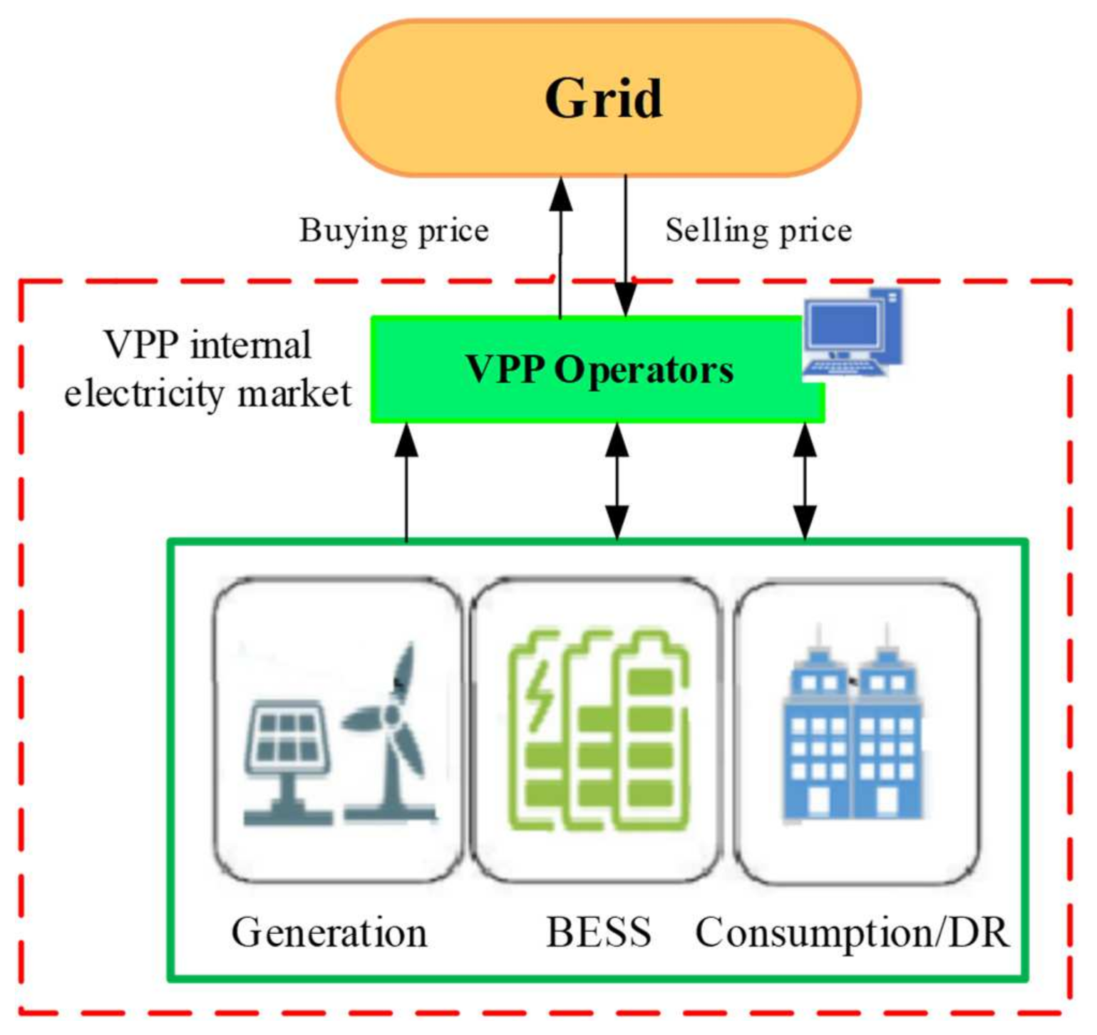
5. VPP Electricity Market Model Description

In this section, we present the VPP’s internal electricity market structure, which includes VPP operators, energy generation, internal electrical consumption, a DR program, and a BESS. The internal generation system encompasses renewable energy sources (i.e., WT and PV generators). The internal electrical consumption system encompasses energy consumers. The BESS charges when there is a low price or consumption and discharges when there is high demand for energy. The VPP operators have a duty to meet consumer demands in the VPP internal electricity market by acquiring energy from the utility grid or obtaining power from internal generators. To relieve supply pressure, the VPP encourages internal electrical consumers to take part in the DR program by load reductions with compensation. By charging and discharging, the BESS acts as a reserve component to efficiently move loads from peak to off-peak times.

According to Figure 2, each consumer in the internal electricity market is supposed to submit the VPP operators with an offer and bid capacity for their load reductions when taking part in a DR program. The internal consumer is ready to minimize energy demand by less than or equal to the required power capacity over a predetermined time for each offer and bid that includes a load reduction capacity with a corresponding bid price. Furthermore, the operational data of WT and PV units, as well as the BESS characteristics, are captured by the VPP operator.

The VPP operators implement an internal electricity market optimization to find the best operational scheme for each component in order to minimize the costs while respecting system constraints. Finally, the VPP discloses the best compensation rates to consumers with matching corresponding load reductions. In addition, the VPP operators also ascertain the quantity of energy that can be supplied by the internal WT and PV generators, as well as the charging/discharging capacities of the BESS.

6. Case Study, Simulation, and Results and Discussion

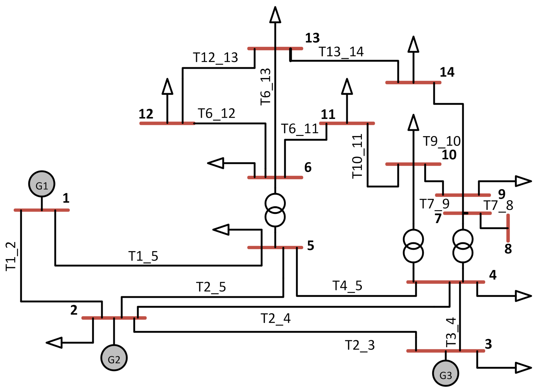
A case study is presented to demonstrate the feasibility of the proposed approach and to validate the simulation studies on a 14-bus distribution system. Figure 3 shows a slightly modified single-line diagram of a 14-bus system. The data associated with the IEEE 14-bus system is included in Appendix A. In this study, we only considered active power generation, while reactive power is out of the scope of this work. Our VPP constitutes two WTs, one PV unit, dispatchable loads, and a BESS. During normal operation, the VPP is connected to the utility grid. Bus 1 is assumed to be a possible location for installing a PV unit, whereas Buses 2 and 3 are supposed to be two feasible locations for the installation of WTs. The power factor of the load buses is assumed to be constant. A BESS is installed at Bus 5 since the BESS was already deployed in the system; therefore, the BESS case problem does not take into account the initial capital cost. The charging/discharging efficiencies of the BESS are supposed to be 95 and 90 percent. The minimum/maximum voltage limits are supposed to be V_min = 0.94 p. u/V_max = 0.95 p. u. In this study, it is anticipated that WTs with a capacity of 660 kW, PV with a capacity of 440 kW, and a storage system with a capacity of 200 kW are installed at their assigned buses. The proposed approach is solved as a nonlinear optimization problem. All relevant data with some modifications have been taken from [14,15] to fit our purpose.

Table 2. Utility cost comparison.

Cases	Total Utility Cost (USD)
A (base case)	33,593,826
B (DR case)	33,487,100
C (BESS case)	33,589,662

shows the results comparison of the three cases of utility cost optimization. The proposed mechanism is implemented in a GAMS environment and solved with a nonlinear model [33,34,35].

6.1. Case 1

The objective function in (10) is used to solve the OPF model for Case 1. Figure 4 shows the corresponding generator commitments at Buses 1, 2, and 3. In Case 1, the total cost to the utility is USD 33,593,826. The cheapest generator of the system is located at Bus 3, as shown in Figure 4. As a result, this generator is used to its full possible capacity to satisfy the VPP internal load demands. The second cheapest generator in the system is located at Bus 2. Consequently, it uses its maximum possible generation capacity for most of the day. However, the generator commitments at Bus 2 fall below the maximum limit for hours 8–13 h. This is due to lower system load demands in this period compared to the rest of the day. In this timeframe, the best option is to fully load the generators at Buses 3 and 1, and the generator at Bus 2 will balance the leftover system load demand to keep the cost minimum.

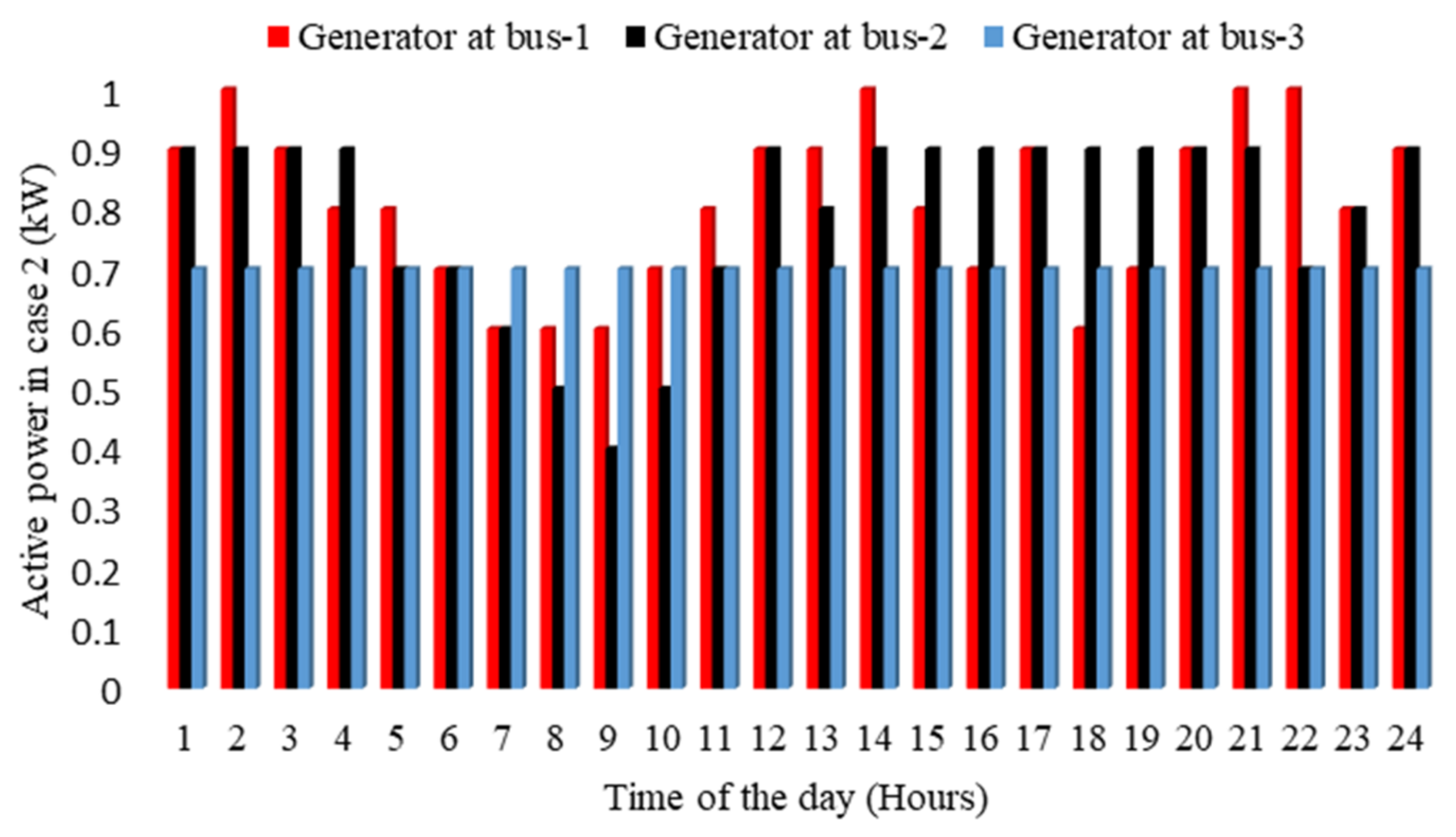
6.2. Case 2

The OPF model is solved for Case 2 using the DR case problem with its associated constraints. Figure 5 shows the corresponding generator commitments at Buses 1, 2, and 3. In the DR case, the total cost to the utility is USD 33,487,100. In the DR case, the load demand of the system will be less as compared to Case 1. This is due to the load curtailment. Therefore, the commitment of the expensive generator at Bus 1 will be lower than it was in Case 1. The commitment of the generator at Bus 3 supplies the most available power at the lowest cost, whereas the generator at Bus 2 usually operates at the maximum possible capacity, except between hours 7 and 13, when it balances the load demand of the system with the generator at Bus 1, keeping the operating cost to a minimum.

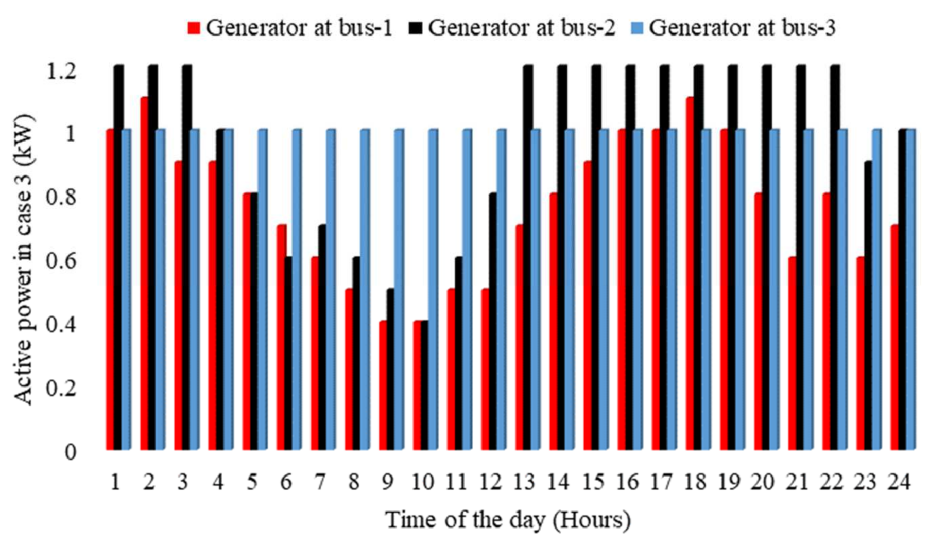
6.3. Case 3

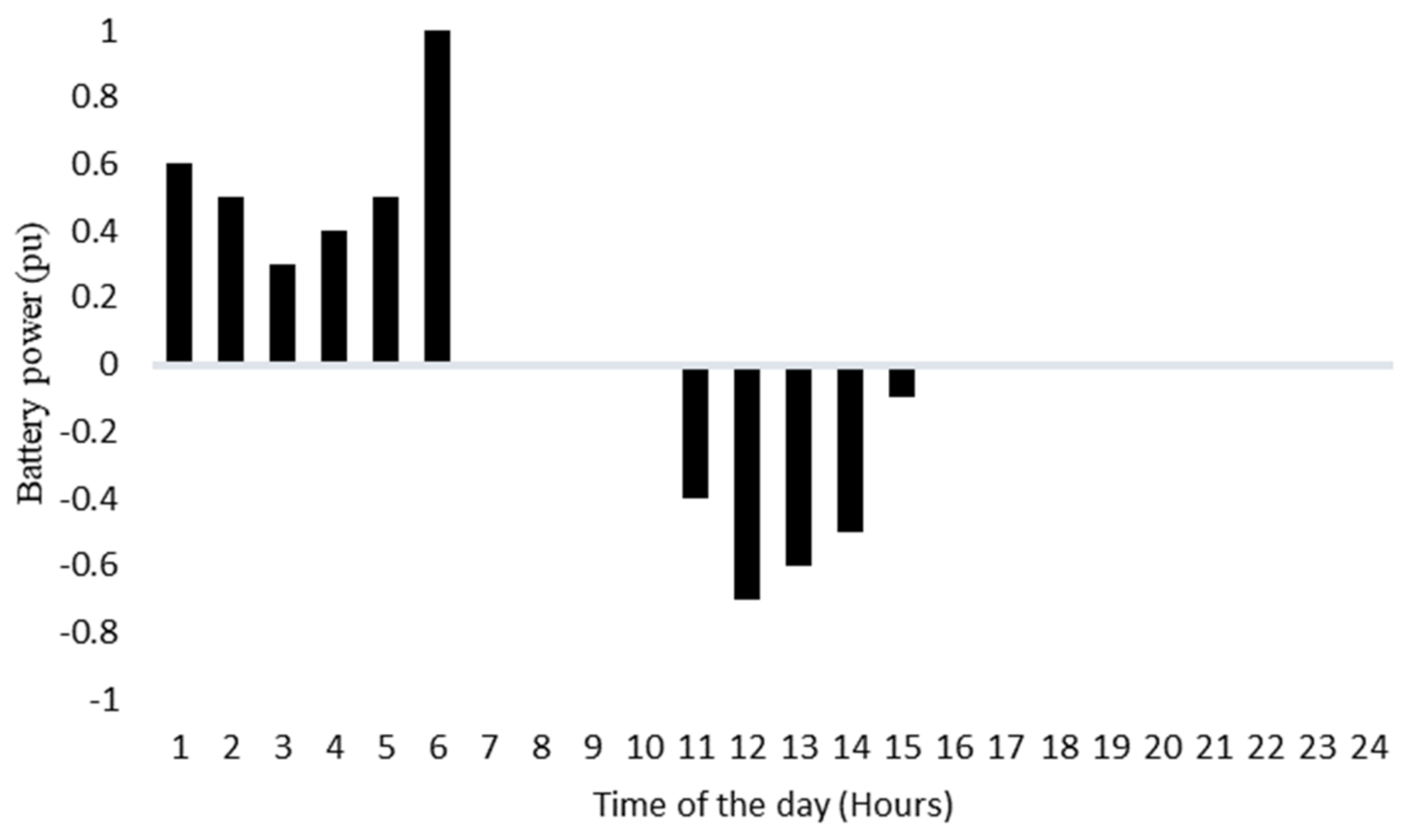
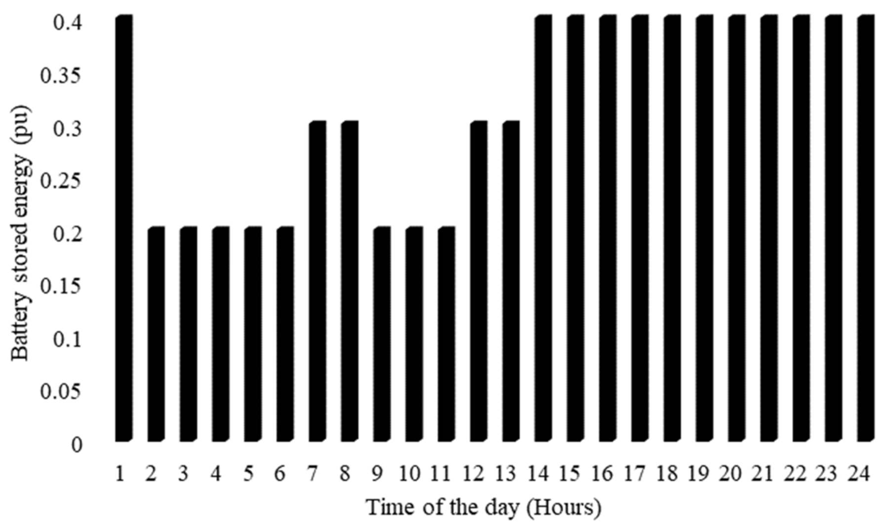
The OPF model is solved in Case 3, using the BESS case problem’s objective function with its related constraints. Figure 6 shows the corresponding generator commitments at Buses 1, 2, and 3. In addition, Figure 7 and Figure 8 show the BESS power and stored energy. In the BESS case, the total cost to the utility is USD 33,589,662. Figure 7 displays the best BESS operation pattern when the aim is cost optimization. The generator commitment in Case3 is identical to that in Case 1, with the exception of the battery’s operational hours. The commitment of the generator will be minimized when the battery is in a state of discharge mode because there will be a decrease in supplying some of the power handled by the battery. This occurs in hours 1–3 when the battery is in a state of charge mode, and the conventional generator commitment exceeds the Case 1 values. During this time period, generators must meet both batteries’ charging power and system demand. The commitment of the generator at Bus 3 supplies the most available power at the lowest cost. The generator at Bus 2 operates at maximum capacity most of the time to meet load demand, except in hours 8–13, when it balances the system demand with the help of the generator at Bus 1, minimizing operational cost.

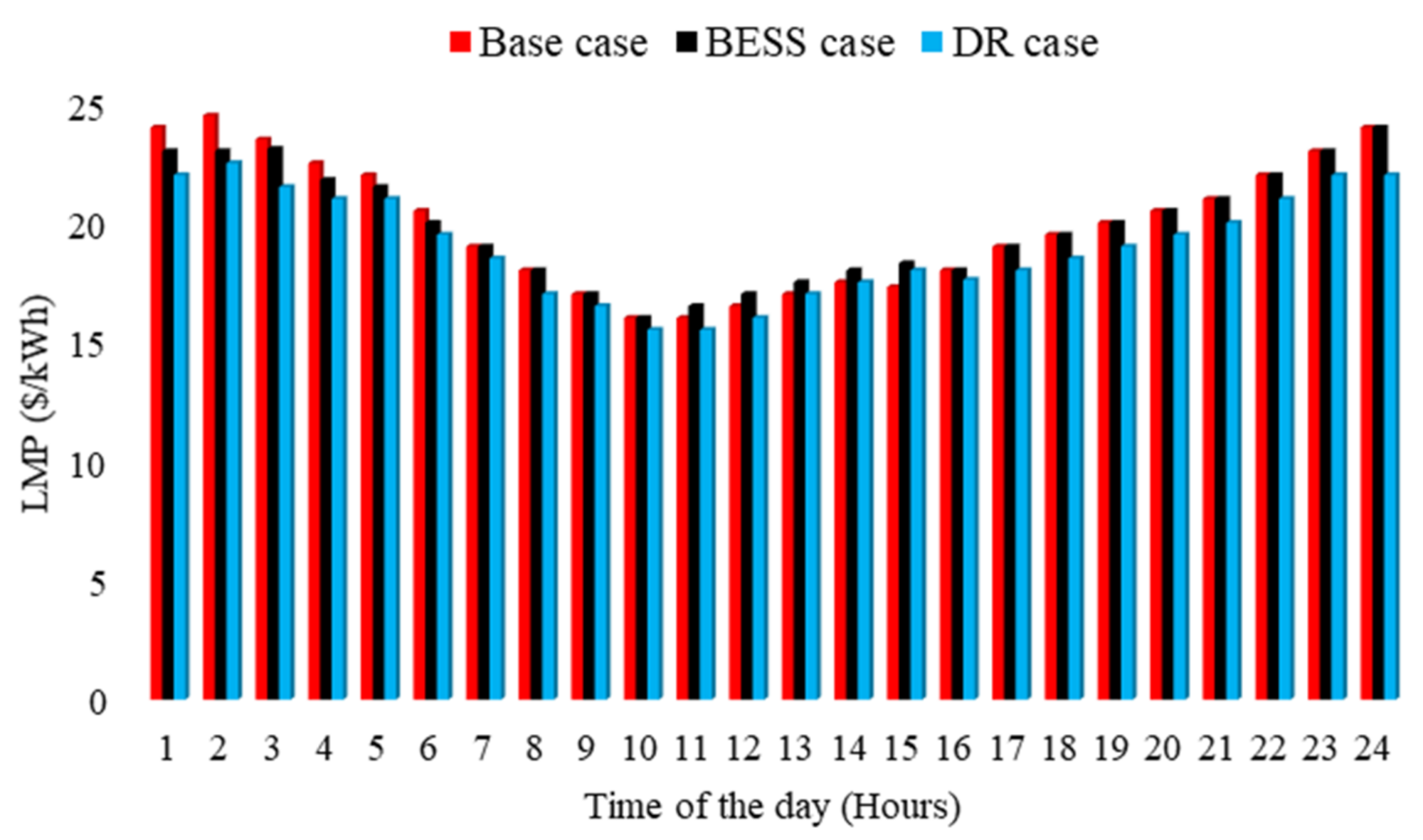
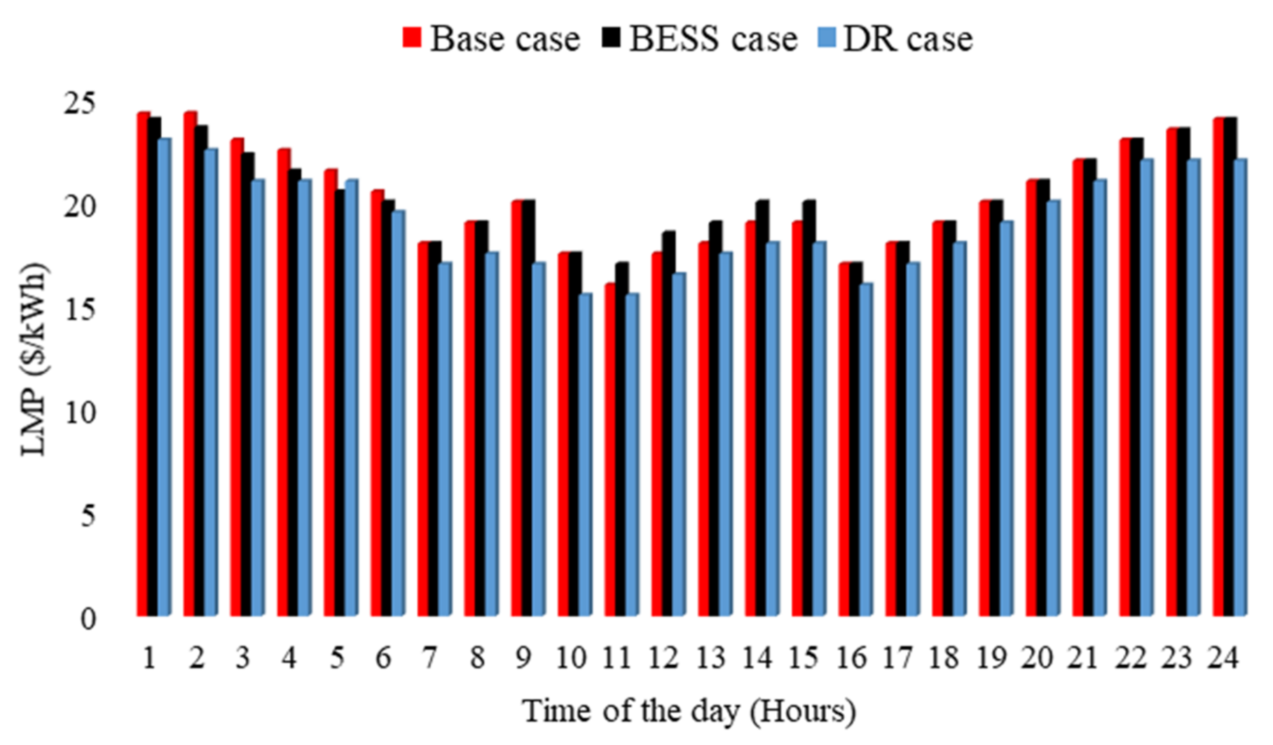
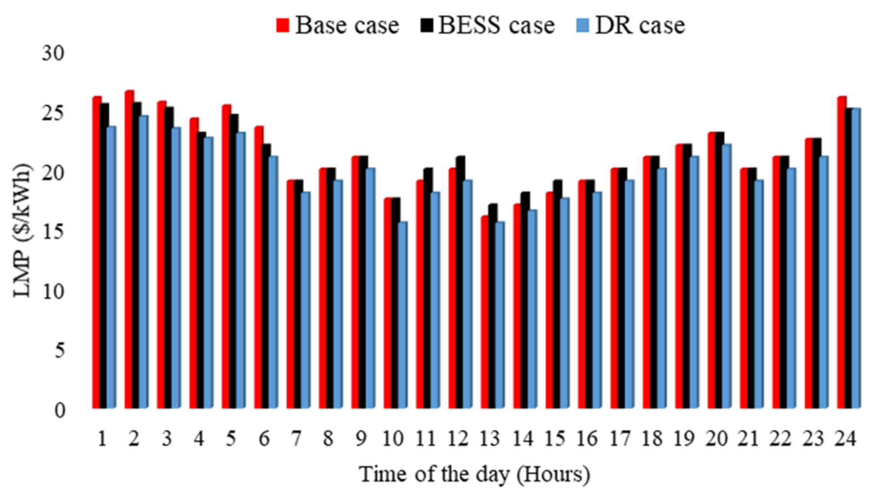
7. Locational Marginal Costs Comparison

A comprehensive comparative study of the locational marginal prices (LMPs) in three different scenarios for Candidate Buses 1–3 is shown in Figure 9, Figure 10 and Figure 11. When the generator commitments in Case 1 (base case) and Case 2 (DR case) for candidate buses are compared, Case 2’s utility advantages outweigh its utility costs, and this is reflected in the overall costs in both cases. This causes the DR case LMPs to be lower than those in the base case, as seen in Figure 9, Figure 10 and Figure 11. Similarly, when comparing Case 1 (base case) and Case 3 (BESS case) for Candidate Buses 1–3, when the battery is not functioning, except during hours 1–3 and 9–12, the generators in both cases have made the same commitment. This shows that the cost incurred is identical. This results in LMPs also being the same in both cases during this timeframe. However, when the battery is charging during hours 9–12 and discharging during hours 1–3, the commitment will be different; therefore, the cost incurred will also be different. As a result, LMPs will differ. The BESS case LMPs are lower as compared to the base case during the discharging phase (1–3), while the LMPs of the BESS case are higher during the charging phase (hours 9–12) as the generation obligations grow to charge the battery and meet the system demand. In order to accomplish the aim of low operating costs, the battery is charged during the timeframe with the least LMPs (hours 9–12).

8. Conclusions and Future Research

The structure of the VPP presented in this study consists of a local distribution network that aggregates renewable generators (i.e., WTs, PVs), DR model, BESS model, and electrical loads. This approach aims to satisfy the criteria of supplying electricity to internal consumers while optimizing utility costs. The findings of the three scenarios are comprehensively compared and analyzed. It was found that implementing a DR program case leads to considerable utility cost savings, which has a direct impact on the LMPs at system candidate buses. As a result, the electricity prices at these candidate buses will be minimum (i.e., Locational marginal prices). Therefore, the proposed approach helps in minimizing utility costs by curtailing peak load demand and thus contributes to the power system stability. Using a BESS model for cost-minimization objectives leads to optimized overall incurred costs and, subsequently, operating costs. The BESS enables VPPs to participate in the balancing market. It features the flexibility to swiftly alter the power output. Therefore, it could be a more cost-effective option for RES curtailment. Furthermore, when the results of the three cases (i.e., base model, DR model, and BESS model) are compared, the DR program is more economical in terms of overall cost reductions and LMPs at specified buses. Therefore, it is obvious that the DR program will have the dominant position, while the BESS model will be marginally dispatched. Other models will be investigated in the future, where a BESS model provides better cost optimization compared to the DR model. For instance, a real-time model might offer BESS as a preferable strategy due to its quick response ability.