Article

Closed-Loop Combustion Optimization Based on Dynamic and Adaptive Models with Application to a Coal-Fired Boiler

1
National Engineering Research Center of Power Generation Control and Safety, School of Energy and Environment, Southeast University, Nanjing 210096, China
2
Shenhua Guohua (Shouguang) Thermal Power Co., Ltd., Shouguang 262714, China
*
Author to whom correspondence should be addressed.
Energies 2022, 15(14), 5289; https://doi.org/10.3390/en15145289
Submission received: 5 June 2022 / Revised: 16 July 2022 / Accepted: 19 July 2022 / Published: 21 July 2022

Abstract

:
To increase combustion efficiency and reduce pollutant emissions, this study presents an online closed-loop optimization method and its application in a boiler combustion system. To begin with, three adaptive dynamic models are established to predict NOx emission, the carbon content of fly ash (Cfh), and exhaust gas temperature (Teg), respectively. In these models, the orders of the input variables are considered to enable them to reflect the dynamics of the combustion system under load changes. Meanwhile, an adaptive least squares support vector machine (ALSSVM) algorithm is adopted to cope with the nonlinearity and the time-varying characteristics of the combustion system. Subsequently, based on the established models, an economic model predictive control (EMPC) problem is formulated and solved by a sequential quadratic programming (SQP) algorithm to calculate the optimal control variables satisfying the constraints on the control and control moves. The closed-loop optimization system is applied on a 600 MW boiler, and the performance analysis is conducted based on the operation data. The results show that the system can effectively increase boiler efficiency by about 0.5%.

1. Introduction

As the main primary energy source of power generation in China, coal will remain dominant for the near future [1]. However, with increasing operating costs and environmental concern, it is necessary for coal-fired power plants to increase combustion efficiency and reduce NOx emission. Against this background, optimizing the combustion conditions of boilers has become a research hotspot.
In recent years, the methodology combining data-driven modeling and optimization algorithms has seized a dominant position in the field of combustion optimization, along with the development of artificial intelligence techniques [2]. The common steps are, firstly, establishing the model of a combustion process, then constructing a performance index related to boiler efficiency or NOx emission, and lastly optimizing the control variables using optimization algorithms. In recent years, many researchers have focused their efforts on the modeling methods [3,4,5,6,7] and optimization algorithms [8,9,10,11,12] of combustion optimization systems. Shi et al. [3] developed artificial neural network (ANN) models of NOx emission and boiler efficiency, and the genetic algorithm (GA) was used to search the optimal control variables. The training samples of the models were obtained by computational fluid dynamics (CFD) simulation and historical operating data. Wang et al. [4] implemented two Gaussian process (GP) models of NOx emission with different numbers of inputs, and then determined the model inputs by comparing the performance of the two models. The optimization of the operation parameters was accomplished via the genetic algorithm (GA).
Li et al. [5] integrated load balance and coal qualities into a support vector machine (SVM) model of NOx emission. The results showed that the optimization based on the new model could provide lower NOx emission and meet load demand at the same time. Tan et al. [6] established a novel extreme learning machine (ELM) model of NOx emission based on the historical data of a 700 MW opposed wall-fired boiler, and harmony search (HS) was exploited to realize NOx emission reduction. Fan et al. [7] presented a novel deep structure using a continuous restricted Boltzmann machine (CRBM) with SVM and kernel principal component analysis (KPCA) was applied to identify steady-state samples. Li et al. [8] proposed a novel Lévy flight vortex search algorithm to tune the adjustable parameters of a boiler to achieve combustion optimization. Zhang et al. [9] developed least squares support vector machine (LSSVM) models for boiler efficiency, NOx emission, and SO2 emission, and used the fruit fly optimization algorithm (FOA) to obtain optimal operation parameters by integrating three objectives into a single performance index function. Zheng et al. [10] applied LSSVM to establish the models of NOx emission and boiler efficiency, and then the utilized multi-objective particle swarm optimization (MO-PSO) algorithm to calculate the optimal solutions. Gu et al. [11] applied integrated clustering based on a K-prototype algorithm for multi-objective optimization in boilers. Niu et al. [12] proposed a case-based reasoning optimization method based on grey relational theory (GR-CBR) and LSSVM models.
In these studies, the models of combustion system were all built offline based on historical data. Although good results have been achieved in short-term simulation tests, the prediction accuracy will decrease over time in field applications because of the time-varying characteristics of the combustion process. Due to unavoidable changes in coal quality and the fouling of heating surfaces, the original fixed models will deviate from the actual characteristics of the combustion process, therefore undermining the effectiveness of the optimization results.
To track the time-varying characteristics of the combustion process, an adaptive model is essential. Smrekar et al. [13] proposed an adaptive modeling method based on forgetting factors and established an auto-regressive model with external inputs for NOx emission. Zhao et al. [14] proposed an online prediction algorithm based on LSSVM. New samples were continuously added and weighted to varying degrees with sampling time during the online operation. On this basis, Gu et al. [15] proposed an adaptive update algorithm for the LSSVM model, i.e., the adaptive least squares support vector machine (ALSSVM), which can incrementally replace old samples and improve the model performance adaptively. The effectiveness of the adaptive modeling algorithm was verified by testing the model of exhaust temperatures over a long period of time. Lv et al. [16] divided the process variations into irreversible and reversible types and then applied ALSSVM to predict the NOx emission. The results showed that the adaptive modeling method could cope with the irreversible model changes that traditional methods cannot solve while maintaining the accuracy of the model for a long time. Zhai et al. [17] combined ALSSVM with the forgotten factor and iterative algorithm, which improved the performance of the prediction model of NOx emission in terms of long-term prediction. However, the above models are static models, which can only reflect the relation between the inputs and the outputs of a combustion system under a steady state, because the time lags from the inputs to the outputs are not considered in these models.
In view of the dynamic modeling of boiler systems, Lu et al. [18] established a dynamic back propagation neural network (BPNN) model using two-step historical values as part of the model inputs. Lv et al. [19] developed a dynamic LSSVM model by considering the current and past values of independent variables as model inputs. The comparison results showed that the dynamic model had a higher prediction accuracy than the steady model in describing the dynamic characteristics of the boiler systems. Some other studies [20,21,22] established dynamic NOx emission models based on the long short-term memory network (LSTM) and achieved dynamic series prediction by retaining the information from previous series. It should be noted that the above dynamic models do not consider adaptive updating, and their prediction accuracy will gradually decrease with the passage of time. Therefore, time-varying and dynamic characteristics must be taken into account simultaneously when establishing a boiler combustion process model, but there is little related work at present.
On the other hand, from the perspective of industrial application, the previous studies are almost in the simulation stage, and some of the systems that have been put into use are mostly open-loop guidance systems. As these systems often need frequent manual operation, it is often unrealistic and difficult to achieve practical results. Therefore, it is necessary to develop a closed-loop combustion optimization control system, combined with the existing combustion control system in the distributed control system (DCS), to automatically adjust combustion according to the current load and coal quality [21].
In this paper, to address the above-mentioned weaknesses, a closed-loop combustion optimization control method is proposed by combining adaptive dynamic models of combustion systems and economic model predictive control (EMPC). Moreover, the proposed method is successfully applied to a 600 MW opposed wall-fired boiler. The rest of this paper is organized as follows. In Section 2, three ALSSVM models of NOx emission, carbon content of fly ash (Cfh), and exhaust gas temperature (Teg) are established. The proposed closed-loop combustion optimization control method based on EMPC is presented in Section 3. Section 4 gives the application results and the performance is analyzed based on the operation data. Conclusions are drawn in Section 5.

2. Dynamic and Adaptive Modeling of the Combustion Process

2.1. Boiler Description

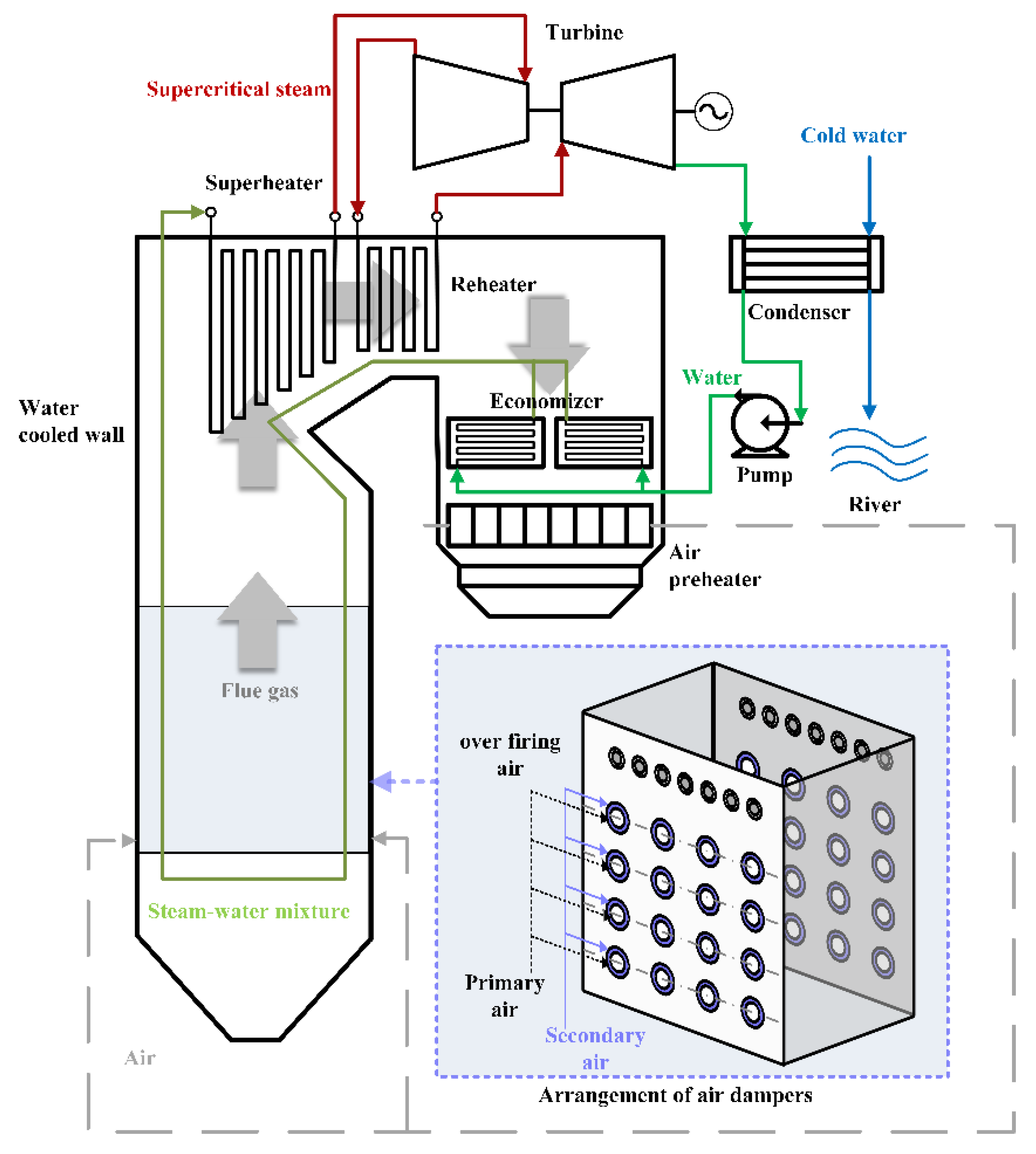
The object of this study is a 600 MW opposed wall-fired ultra-supercritical boiler. A schematic diagram of this HG-1987/25.4-YM1 boiler is shown in Figure 1.
A total of thirty-two center-feed low NOx swirl burners were equipped on the front and back walls of the furnace (four on the front wall and four on the back wall at the same height). The innermost layer of the burner was the primary air mixed with pulverized coal, and the secondary air was distributed concentrically outside of the primary air. Above the uppermost layer of the burner, one layer of over fire air (OFA) dampers was divided into two groups, with seven on each wall. This boiler was equipped with four double-inlet and double-outlet steel ball mills. Under the boiler maximum continuous rating (BMCR) condition, all four coal mills were put into operation. Each coal mill supplied pulverized coal to eight burners on the same layer. The main design parameters of the boiler are listed in Table 1. The mixture of anthracite and bituminous coal was combusted in this plant, and the properties of the coal are shown in Table 2.
In order to evaluate the combustion situation more comprehensively and minimize the heat loss due to unburned carbon (q4) during optimization, the boiler was equipped with a real-time measurement device for the carbon content of fly ash. The device was installed in the tail flue of the boiler. In each operating cycle, the sampling system took a fixed mass of ash sample, and the weighing, burning, cooling, and discharging operations were performed to calculate the carbon content in the ash sample. The entire sampling and analysis process took about thirty minutes; thus, the measured value of carbon content in fly ash could be obtained every thirty minutes.

2.2. Data Preparation

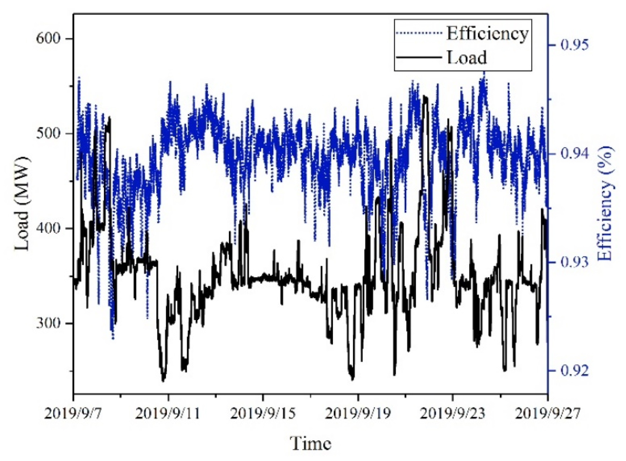
More than 80,000 sets of historical operation data, spanning 20 days, were acquired from the supervisory information system (SIS) with sampling intervals of 20 s. Eleven variables were employed as the model inputs according to the practical condition of this boiler, including ten control variables (four offset values of coal-feed rate, four layers of secondary air damper opening, one layer of OFA damper opening and oxygen content setpoint after the economizer), and one state variable (unit load). Several indicator parameters were obtained to calculate boiler efficiency in real time based on the Chinese GB10184-88 standard, as shown in the Appendix A. After eliminating noise and the outliers, the final dataset was obtained. The data regarding unit load and boiler efficiency are shown in Figure 2.

2.3. Modeling of Boiler Combustion System

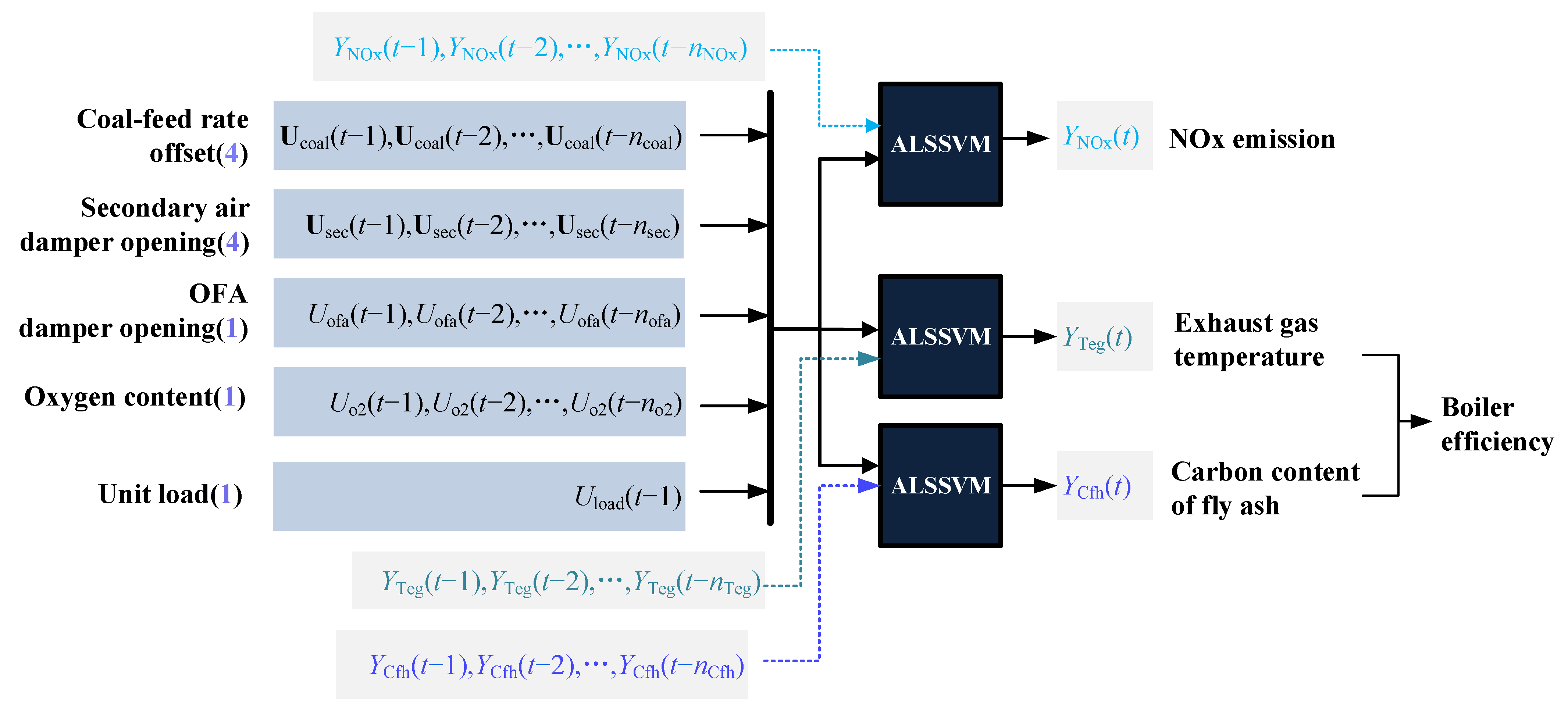
Three models were established to characterize the combustion state of the boiler, including NOx emission, exhaust gas temperature (Teg), and carbon content of fly ash (Cfh). Unlike the common structure of combustion models, dynamic modeling and adaptive update methodologies were considered.
Firstly, the current values and previous sequences of the selected variables were considered as the model inputs to describe the dynamic characteristics of the combustion process. Then, three ALSSVM models were established between inputs and three outputs, and the boiler efficiency was calculated by the formula introduced in the Appendix A. The parameters of each model were adaptively updated according to the newly acquired data during operation.

2.3.1. Dynamic Model Structure

As a complex nonlinear dynamic system with heavy response delays, the output parameters of the boiler combustion system will go through a relatively long transient process to reach a new stable state after the manipulated variables are changed. Thus, this paper employs dynamic modeling to improve the model accuracy during load variation by considering the delay orders of the input and output variables.
The model structure of the boiler combustion system is shown in Figure 3. The NOx emission model can be described by (1), and the other two models are similar.
Y ^ ( t ) = f NOx ( x ( t ) ) x ( t ) = [ U coal ( t 1 ) , , U coal ( t n coal ) , U sec ( t 1 ) , , U sec ( t n sec ) , U ofa ( t 1 ) , , U ofa ( t n ofa ) , U o 2 ( t 1 ) , , U o 2 ( t n o 2 ) , U load ( t 1 ) , Y ( t 1 ) , , Y ( t n NOx ) ]
where t is the current moment; f NOx ( ) is the LSSVM regression function of NOx emission; Y ^ ( ) is the predictive output by the function; Y ( ) is the historical value of the output; U coal ( ) , U sec ( ) , U ofa ( ) , U o 2 ( ) , U load ( ) represent the values of coal feed rate offset, secondary air damper opening, OFA damper opening, oxygen content after the economizer and unit load at a given moment, respectively; n coal , n sec , n ofa , n o 2 , n load denote the delay order of these input variables; and n NOx , n Teg , n Cfh are the delay orders of the output variables including NOx emission, Teg and Cfh.

2.3.2. Combustion Process Modeling Using ALSSVM

The model inputs x and corresponding outputs Y at the same moment form the set of a training sample. Then, the training dataset can be expressed as T = { ( x 1 , Y 1 ) , , ( x l , Y l ) } , which consists of l samples with d-dimension inputs x i R d and outputs Y i R , i = 1 , 2 , , l . The decision function f ( x ) of the LSSVM regression model can be obtained by the Lagrangian multiplier method, as follows:
f ( x ) = k = 1 l α k K ( x k , x ) + b
where α k is the Lagrangian multiplier corresponding to the kth training sample x k ; K ( , ) is the radial basis kernel function (RBF); and b is a bias. The above model parameters can be obtained by (3).
{ α = H - 1 Y - H - 1 e e T H - 1 Y e T H - 1 e b = e T H - 1 Y e T H - 1 e
where α is denoted as α = [ α 1 , α 2 , , α l ] T   Y is the output vector of the training dataset denoted as Y = [ Y 1 , Y 2 , , Y l ] T ; e is an l-dimension identity column vector; and H is the feature matrix of the LSSVM which is written as (4) and satisfies the equation relationship shown in (5).
H = [ K ( x 1 , x 1 ) + 1 2 c K ( x 1 , x 2 ) K ( x 1 , x l ) K ( x 2 , x 1 ) K ( x 2 , x 2 ) + 1 2 c K ( x 2 , x l ) K ( x l , x 1 ) K ( x l , x 2 ) K ( x l , x l ) + 1 2 c ]
H [ b α 1 α 2 α l ] = [ 0 Y 1 Y 2 Y l ]
where c is the penalty parameter, and the RBF kernel function K ( , ) can be expressed as follows:
K ( x i , x j ) = exp ( - x i x j 2 2 δ 2 )
where δ is the kernel parameter.
Through the above calculations, the original training of the LSSVM model can be accomplished. Furthermore, when the accuracy of the regression model is unsatisfied, the initial support vectors should be replaced with newly obtained operating data and updated model parameters [15]. The updating process is introduced as follows:
First, find the ith sample ( x i , Y i ) in the original training dataset which is closest to the new operating data ( x new , Y new ) , as shown in (7):
i = arg ( min k = 1 , l x new x k )
Then, exchange the components between the ith and the lth line of H and then between the ith and the lth row. After that, a new matrix H 1 is obtained as follows:
H 1 = I R i R l H I L i L l = [ K ( x 1 , x 1 ) + 1 2 c K ( x 1 , x l ) K ( x 1 , x i ) K ( x l , x 1 ) K ( x l , x l ) + 1 2 c K ( x l , x i ) K ( x i , x 1 ) K ( x i , x l ) K ( x i , x i ) + 1 2 c ]
where I R i R l is obtained by interchanging components between the ith and the lth line of an identity matrix, and I L i L l is obtained by the same interchanging but between the row components. In terms of matrix theory, the transformation from H to H 1 can be accomplished by pre-multiplying I R i R l and post-multiplying I L i L l .
For partition H 1 in (9), where G is composed of the first l − 1 lines and l − 1 rows of H 1 , the column vector g i is composed of the first l − 1 rows in the last line of H 1 .
H 1 = [ G g i g i T K ( x i , x i ) + 1 2 c ]
The inverse of matrix H1 can be calculated as
H 1 1 = [ h 11 h 12 h 21 h 22 ] = I R i R l H 1 I L i L l
Accordingly, the inverse of the new feature matrix H2 should be computed as
H 2 - 1 = [ G - 1 + G - 1 g n e w r new - 1 g n e w T G - 1 - G - 1 g n e w r new - 1 - r new - 1 g n e w T G - 1 r new - 1 ]
where the inverse of G is calculated by (15), and the denotations of g n e w , k new , r new are shown in (12)–(14), respectively.
g n e w = [ K ( x 1 , x new ) , , K ( x i 1 , x new ) , K ( x l , x new ) , K ( x i + 1 , x new ) , , K ( x l 1 , x new ) ] l × 1 T
k new = K ( x new , x new ) + 1 2 c
r new = k new g n e w T G - 1 g n e w
G 1 = h 11 h 12 h 22 1 h 21
Then, the new model parameters α * and b * can be determined using (16), where Y * = [ Y 1 , , Y i 1 , Y l , Y i + 1 , Y l 1 , Y new ] T is the new output vector of the model learning dataset, which is obtained by replacing the ith element Yi in the original output vector with the lth one Yl and the lth element Yl with the output Ynew of the new operating data.
{ α * = H 2 - 1 Y * - H 2 - 1 e e T H 2 - 1 Y * e T H 2 - 1 e b * = e T H 2 - 1 Y * e T H 2 - 1 e

2.4. Model Parameter Determination

The basic method of modeling is shown in the previous section. After that, two types of model parameters need to be determined.
The first type are the hyper-parameters of the ALSSVM models, including the kernel parameter δ and penalty parameter c. Ten-flod cross-validation can be used to determine these parameters. The training dataset is divided into 10 subsets equally. Each of these subsets are removed in turn from the complete training data and the model is trained based on the remaining data. The removed subset is used as testing data. The model accuracy is measured by the root mean square error (RMSE) index (17).
RMSE = 1 N k = 1 N ( y y ˜ ) 2
where y and y ˜ are the actual and predictive values, and N is the number of data samples.
For each value of [ δ , c ] in the search scope, a 10-fold cross-validation is performed to calculate the average value of RMSE. The parameters corresponding to the minimal average value of RMSE were finally used to construct the combustion models.
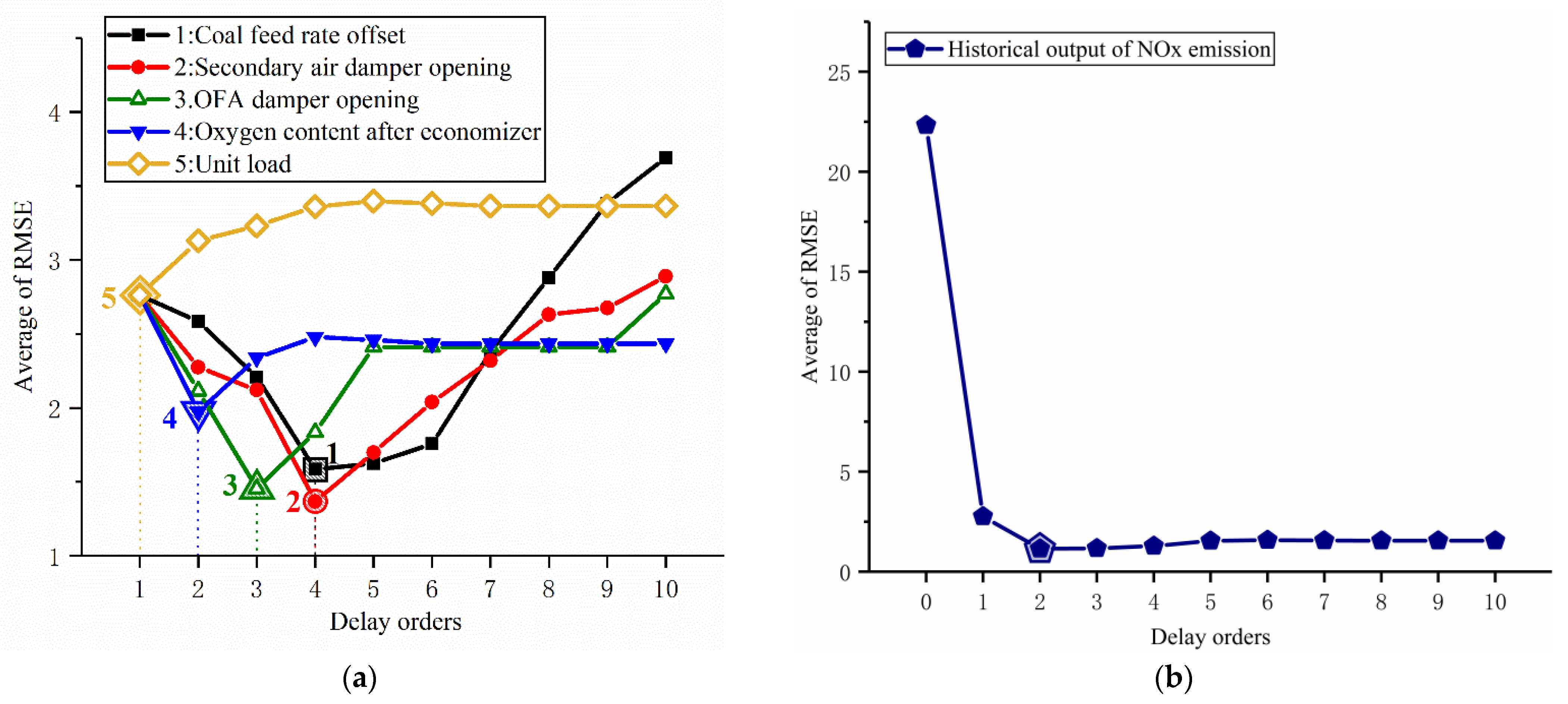
The second type of parameters are the delay orders of the model inputs. For each model, there are six kinds of delay orders to be determined: n coal , n sec , n ofa , n o 2 , n load and the output order n NOx , n Teg or n Cfh . Actually, the best way to acquire this type of parameter is to perform a single-variable disturbance experiment on the boiler. However, this is very time-consuming, and will affect the normal operation of the boiler. Thus, 10-fold cross-validation is also used to find the combination of delay orders in this paper.

3. Closed-Loop Combustion Optimization Based on Economic Model Predictive Control

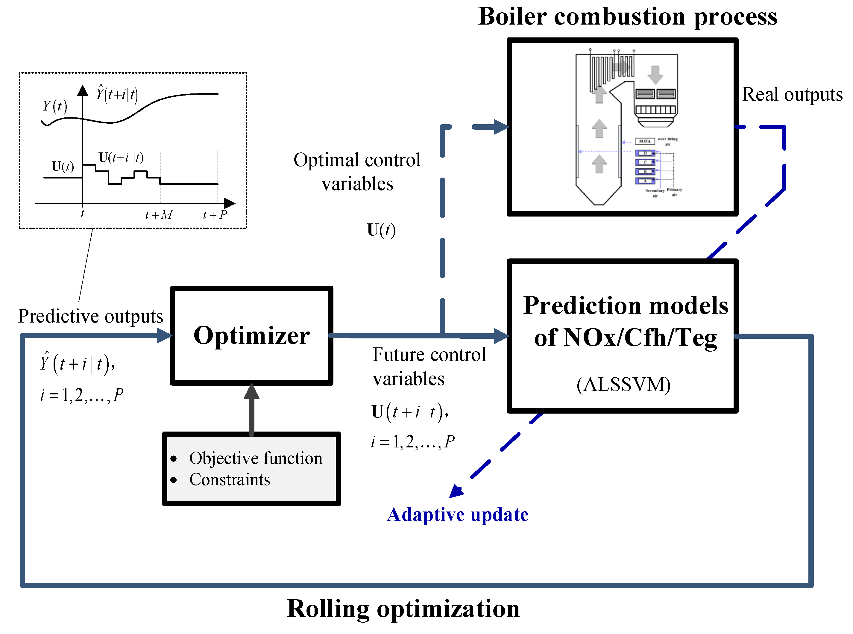
The overall structure of the closed-loop system is shown in Figure 4. On the basis of the above models, an economic model predictive control (EMPC) problem is formulated, as shown in (18), which aims to improve boiler efficiency while reducing NOx emission in a future period.
min U ( t ) J = w 1 i = 1 P Y ^ NOx ( t + i | t ) w 2 i = 1 P Y ^ eff ( t + i | t )
s . t . min U U ( t ) max U , t
min Δ U Δ U ( t ) max Δ U , t
  s u m ( U coal ( t ) ) = 0 , t
where w1 and w2 are the weighting coefficients of NOx emission and boiler efficiency representing the focus of the optimization; t is the current moment and t + i is the future ith moment; Y ^ NOx ( t + i | t ) and Y ^ eff ( t + i | t ) are the predictive sequences of outputs in the range of prediction horizon P; and U ( t ) is the vector of control variables with a control horizon M, which contains four kinds of model inputs, as shown in (22). The magnitude and rate constraints of the control inputs are considered in (19) and (20), respectively. The equality constraint (21) on coal feed rate is set to avoid the impact on unit load when optimizing the combustion. Thus, the four offsets of the coal feed rate should add up to zero.
U ( t ) = [ U coal T ( t | t ) , , U coal T ( t + M 1 | t ) , U sec T ( t | t ) , , U sec T ( t + M 1 | t ) , U ofa ( t | t ) , , U ofa ( t + M 1 | t ) , U o 2 ( t | t ) , , U o 2 ( t + M 1 | t ) ] T
The process of predicting outputs is shown as the dotted box in Figure 4. The established ALSSVM prediction models are used to forecast the future P-step outputs of the combustion system. The predicted sequence of outputs Y ^ ( t + i | t ) , i = 1 , 2 , , P depends on the input and output values at current time t, and on the set of future control variables U ( t ) . Taking the model of NOx emission, for example, the multi-step-ahead sequence of outputs can be predicted using (23).
Y ^ ( t + i | t ) = f NOx [ x ^ ( t + i 1 | t ) ] , 1 i P x ^ ( t + i 1 | t ) = [ U coal ( t + i 1 | t ) , , U coal ( t + i n coal | t ) , U sec ( t + i 1 | t ) , , U sec ( t + i n sec | t ) , U ofa ( t + i 1 | t ) , , U ofa ( t + i n ofa | t ) , U o 2 ( t + i 1 | t ) , , U o 2 ( t + i n o 2 | t ) U load ( t 1 ) , Y ^ ( t + i 1 | t ) , , Y ^ ( t + i n NOx | t ) ]
where f NOx ( . ) represents the ALSSVM model of NOx emission. Likewise, it is also possible to perform multi-step prediction of the other two outputs.
The optimization problem (18) is solved in a receding horizon manner by using the sequential quadratic programming (SQP) algorithm. The SQP algorithm decomposes the original problem into a series of sub-problems which can be solved by quadratic programming, so it is very effective for nonlinear constraint optimization problems [23,24].
This closed-loop combustion optimization method can cope well with load and coal quality variations, as the developed ALSSVM prediction models can be updated automatically based on prediction errors. The advantage is that no new online coal quality measurement equipment is required (online coal quality measurement is currently technically difficult) and the disadvantage is that there is a certain lag in combustion adjustment.

4. Application Results

Based on the above methodology, a combustion optimization system was designed and put into operation in a 600 MW coal-fired boiler. Considering the characteristics of the combustion system and the time required for adaptive the update, the calculation interval was set to 20 s. A large amount of data were recorded during operation. The modeling and optimization performance can be evaluated with these operating data.

4.1. Modeling Results

4.1.1. Combustion Process Modeling Using ALSSVM

As described above, there are three dynamic models established in this work based on LSSVM. One thousand sets of samples, which uniformly covered all operating conditions of the boiler, were selected as the training dataset after normalization and centralization. Based on the training dataset, two types of model parameters could be determined by the process introduced in Section 2.4.
The kernel parameter and penalty parameter were searched in the ranges of [0.1, 3] and [100, 5000]. The final parameters are shown in Table 3.
The search scope of delay orders was [1, 6]. The input orders of the three models were optimized and the results are shown in Table 4.
Taking the NOx model as an example, incremental analyses of the single variables were conducted to verify the effect of order optimization. We changed the order of one variable at a time and fixed the order of other variables to 1. The analysis result of n coal , n sec , n ofa , n o 2 , n load is shown in Figure 5a and the delay order of each variable corresponding to the minimum average RMSE is consistent with Table 4.
In particular, an incremental analysis was performed on the historical output n NOx , and the results are shown in Figure 5b. The zero order represents the steady-state model that no historical output was added to for the model input. It can be seen that the accuracy of the model was greatly improved after taking the historical outputs as the model inputs in the dynamic modeling of the boiler combustion process.

4.1.2. Model Prediction Accuracy

The predictive models with the above parameters were verified by the actual operation data. Figure 6a–c show the prediction accuracy of the three models over a long period of time. It can be seen from the figures that the trends of the predicted values of the three models were consistent with the actual values, and most of the prediction errors were within three small ranges of ±10 mg/m3, ±0.1 °C, and ±0.3%, respectively. The results indicate that the three models have high accuracy and can correctly reflect the characteristics of boiler combustion systems.

4.1.3. Verification of Dynamic and Adaptive Modeling Methodology

Furthermore, several simulation experiments were conducted to verify the effectiveness of the dynamic modeling and adaptive update methodology.
Taking the model of NOx emission as an example, four models were established by different modeling methods based on the same training dataset, i.e., Model 1 (dynamic + ALSSVM), Model 2 (dynamic + LSSVM), Model 3 (steady-state + ALSSVM), and Model 4 (steady-state + LSSVM). The operation data shown in Figure 6 were used to test the model performance. The comparison results are shown in Figure 7. It is clear that Model 1 had the highest accuracy compared with the other three models. The absolute prediction error of Model 1 was within a range of [0, 9] mg/m3. Its variation was also obviously smaller than that of the other three models. These results show that modeling accuracy can be significantly improved by considering the dynamic and time-varying characteristics of the boiler combustion process.

4.2. Industrial Application

The proposed closed-loop combustion optimization system was applied to a 600 MW boiler.
Figure 8 gives the results after the combustion optimization system was put into operation under a steady load of 290 MW at the time of 01:23. It can be seen from the figure that the boiler efficiency improved by about 0.5%. The improvement was mainly owing to the decrease in the carbon content of fly ash and the exhaust temperature. Meanwhile, the NOx emission was reduced by about 100 mg/m3.

5. Conclusions

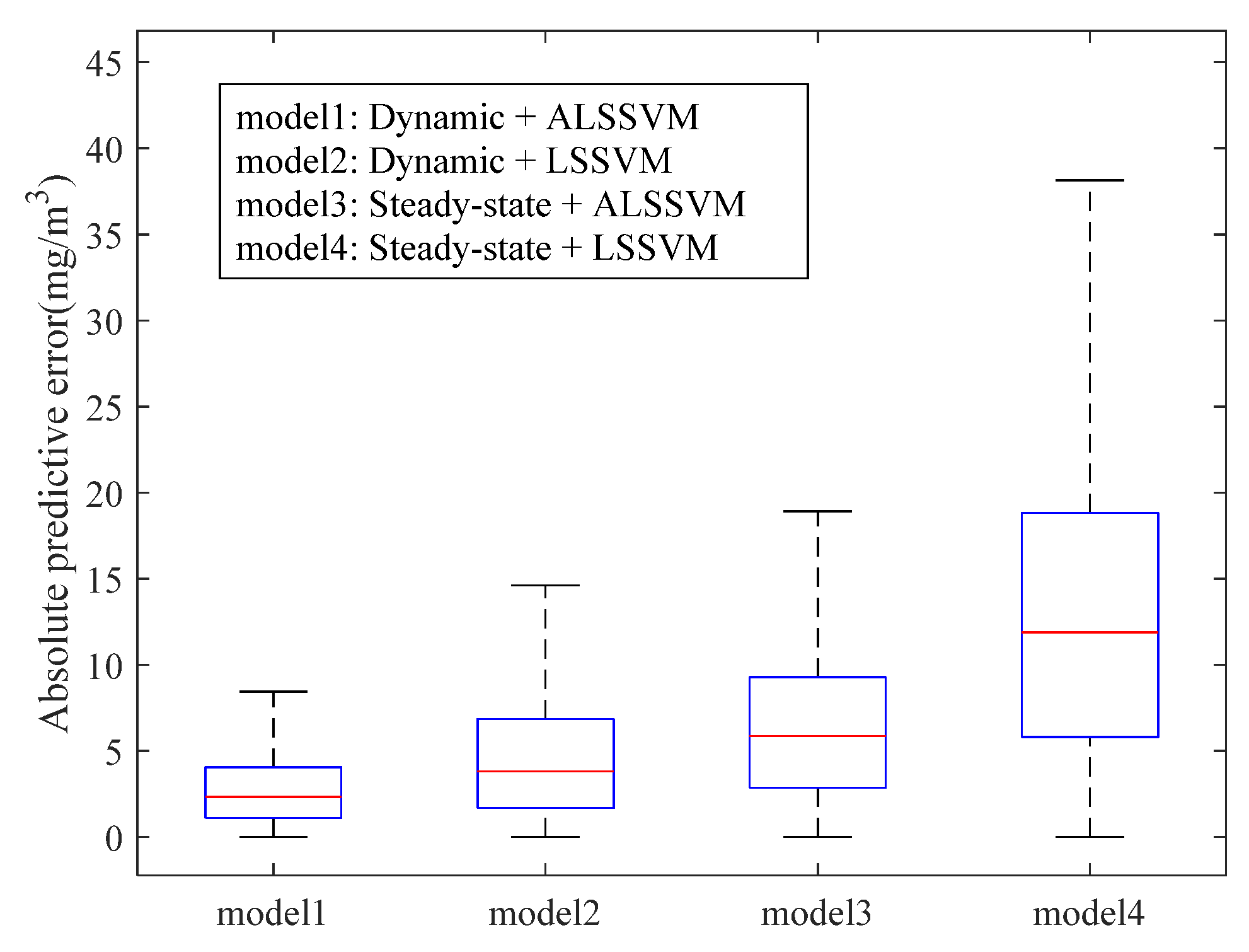
Considering the dynamic and time-varying characteristics of the boiler combustion process, the combustion system model established in this paper is presented with two main improvements compared with other related work: dynamic modeling and adaptive update methodologies.
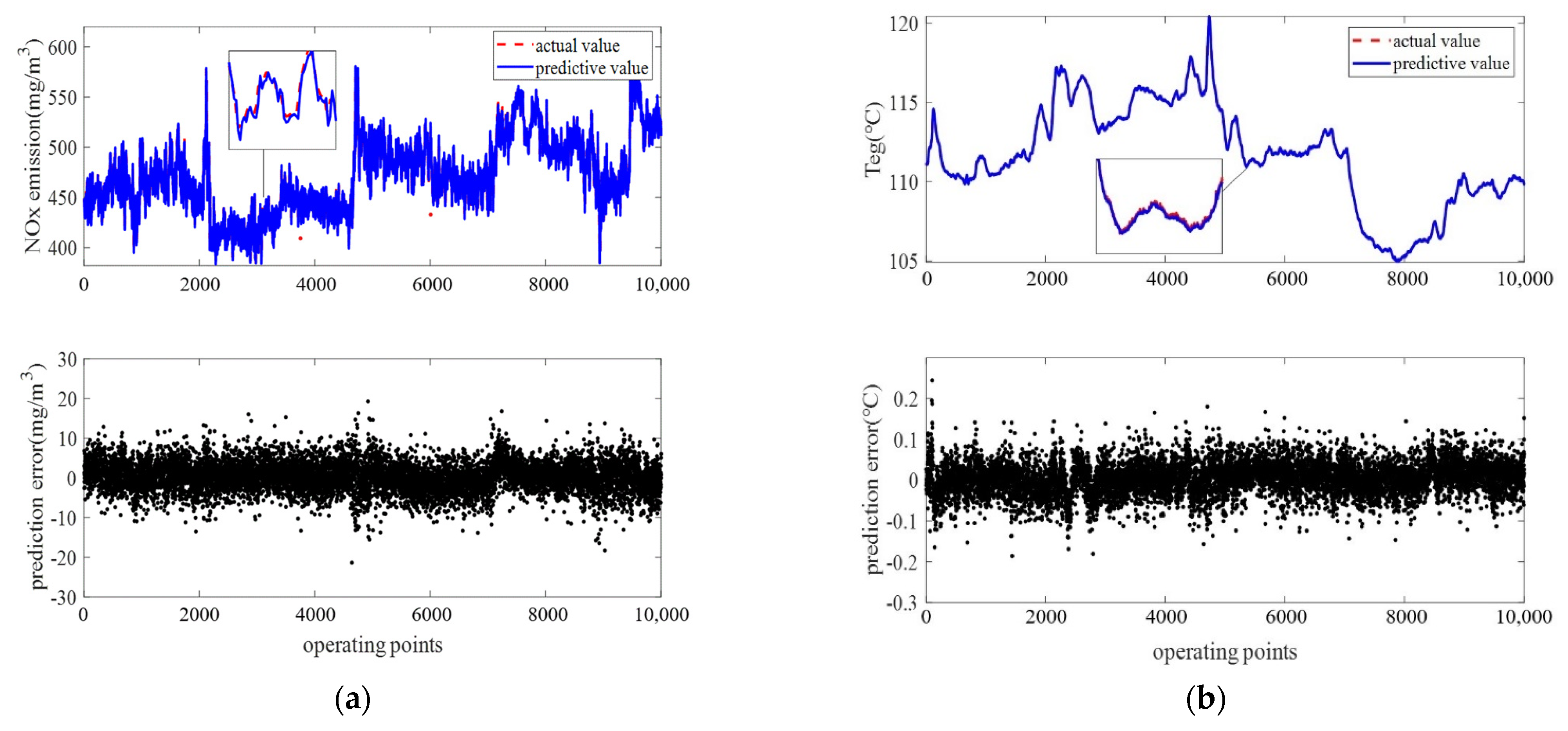
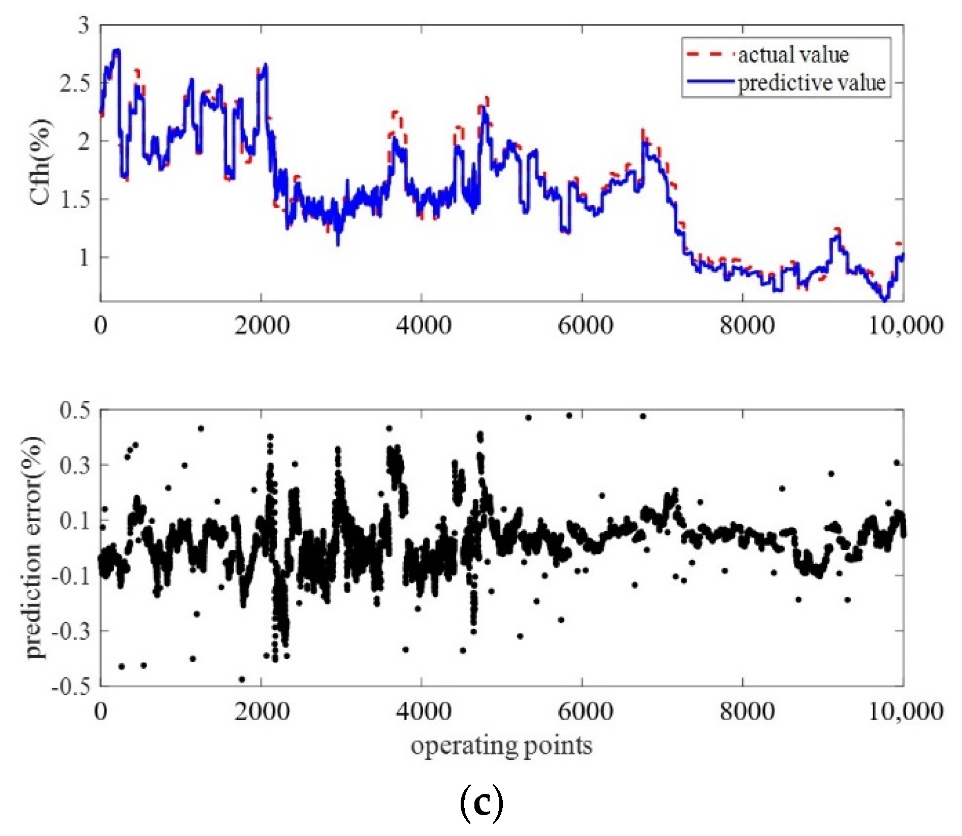
First, the current values and previous sequences of the selected variables were considered as the model inputs to describe the dynamic characteristics of the combustion process. Second, ALSSVM models were updated adaptively based on the operating data, and proved to be more accurate over a long period of operation time.
The effectiveness of the optimization system, which was designed based on the established models, was proven by the closed-loop operation in a 600 MW unit. The actual operation data prove that the system can effectively improve boiler combustion condition and increase efficiency by about 0.5%.
The new closed-loop combustion optimization control system based on the ALSSVM models enables boiler combustion to automatically adapt to changes in load and coal quality, improving boiler efficiency and reducing the workload of operators. It should be noted that although this research is aimed at opposed wall-fired boilers, it can easily be extended to other furnace types, such as tangentially fired boilers, with appropriate modifications to the input variables.

Author Contributions

Conceptualization, Y.L.; Data curation, P.H.; Funding acquisition, Y.L.; Investigation, C.Z. and P.H.; Methodology, C.Z.; Software, P.H.; Writing—original draft, C.Z.; Writing—review & editing, Y.L. All authors have read and agreed to the published version of the manuscript.

Funding

This research was funded by National Key Technology Research and Development Program of China, grant number 2015BAA03B02 and National Natural Science Foundation of China, grant number 51476027.

Institutional Review Board Statement

Not applicable.

Informed Consent Statement

Not applicable.

Data Availability Statement

Data available on request.

Conflicts of Interest

The authors declare no conflict of interest.

Nomenclature

Youtput variable
Uinput variable
tcurrent moment
fregression function
ndelay order of input variable
Hfeature matrix
bregression model bias parameter
Kradial basis kernel function
xinput vector
cpenalty parameter
wweighting coefficient
Pprediction horizon
Mcontrol horizon
Subscripts
coalcoal feed rate offset
secsecondary air damper opening
ofaover fire air damper opening
o2oxygen content after economizer
loadunit load
NOxNOx emission
Tegexhaust gas temperature
Cfhcarbon content of fly ash
effboiler efficiency
Greek symbols
αLagrangian multiplier
σkernel parameter
ηboiler efficiency
Abbreviations
EMPCeconomic model predictive control
SQPsequential quadratic programming
RBFradial basis kernel function
ALSSVMadaptive least square support vector machine
RMSEroot mean square error

Appendix A

In order to calculate the boiler efficiency, the anti-heat balance method was used here as:
η = 100 ( q 2 + q 3 + q 4 + q 5 + q 6 )
where η represents the boiler efficiency and q 2 , q 3 , , q 6 are the five parts of heat loss, which are introduced as follows:
(a)
q2: heat loss due to exhaust gas.
q 2 = Q 2 gy + Q 2 H 2 O Q net , ar × 100
where Q 2 gy is the sensible heat loss of dry gas loss calculated by (A3); Q 2 H 2 O is the sensible heat loss of vapor calculated by (A8); and Q net , ar is the net calorific value as the received basis shown in Table 2.
Q 2 gy = V gy C p . gy ( T eg T 0 ) = ( V gy 0 + ( β 1 ) V gk 0 ) C p . gy ( T eg T 0 )
In (A3), V gy is the dry flue gas volume produced per kilogram of fuel, which is calculated by theoretical dry air volume V gk 0 , theoretical dry flue gas volume V gy 0 and excess air coefficient β , as shown in (A4)–(A6) respectively. T eg is the exhaust gas temperature and T 0 is the ambient temperature. C p . gy represents the average specific heat of dry flue gas at constant pressure, which can be estimated by (A7). [ C P . CO 2 , C P . O 2 , C P . CO , C P . N 2 ] and [ C O 2 , O 2 , C O , N 2 ] are the specific heat and volume fractions of the corresponding gases in the exhaust gas, respectively.
V gk 0 = 0.089 ( C ar + 0.375 S ar ) + 0.265 H ar 0.0333 O ar
V gy 0 = 1.866 × C + 0.375 S ar 100 + 0.79 V gk 0 + 0.8 N ar 100
β = 21 21 O 2
C p . gy = C P . CO 2 C O 2 + C P . O 2 O 2 + C P . CO C O + C P . N 2 N 2 100
Q 2 H 2 O = V H 2 O C p . H 2 O ( T eg T 0 )
In (A8), V H 2 O is the vapor volume produced per kilogram of fuel, which is obtained by (A9). C p . H 2 O is the specific heat of vapor at constant pressure.
V H 2 O = 1.24 ( 9 H ar + M ar 100 + 1.293 β V gk 0 d k )
where H ar , M ar are the coal parameters listed in Table 2 and d k is the absolute humidity of the air, which can be set to a constant value according to the local weather condition.
  • (b) q3: heat loss due to unburned gases.
q 3 = V gy × 126.36 × C O Q net , ar × 100
where C O is the volume fraction of CO in the exhaust gas.
  • (c) q4: heat loss due to unburned carbon.
q 4 = 337.27 × A ar Q net , ar C fh 100 C fh
where Q net , ar and A ar are the coal parameters. C fh is the carbon content of fly ash value measured by the real-time measurement device.
  • (d) q5: heat loss due to radiation.
Take the constant value 0.3% according to the boiler instructions.
  • (e) q6: heat loss due to sensible heat in ash.
q 6 = A ar Q net , ar ( T eg T 0 ) C fh 100 C p . fh
where C p . fh is the specific heat of fly ash.

References

  1. Mischke, P.; Karlsson, K.B. Modelling tools to evaluate China’s future energy system—A review of the Chinese perspective. Energy 2014, 69, 132–143. [Google Scholar] [CrossRef] [Green Version]
  2. Xi, Y.; Kun, L.; Kai, W.; IOP. Summary of Research and Development of Intelligent Combustion Optimization System. In Proceedings of the 2019 3rd International Workshop on Renewable Energy and Development, Guangzhou, China, 8–10 March 2019. [Google Scholar]
  3. Shi, Y.; Zhong, W.; Chen, X.; Yu, A.B.; Li, J. Combustion optimization of ultra supercritical boiler based on artificial intelligence. Energy 2019, 170, 804–817. [Google Scholar] [CrossRef]
  4. Wang, C.; Liu, Y.; Zheng, S.; Jiang, A. Optimizing combustion of coal fired boilers for reducing NOx emission using Gaussian Process. Energy 2018, 153, 149–158. [Google Scholar] [CrossRef]
  5. Li, Q.; Yao, G. Improved coal combustion optimization model based on load balance and coal qualities. Energy 2017, 132, 204–212. [Google Scholar] [CrossRef]
  6. Tan, P.; Xia, J.; Zhang, C.; Fang, Q.; Chen, G. Modeling and reduction of NOX emissions for a 700 MW coal-fired boiler with the advanced machine learning method. Energy 2016, 94, 672–679. [Google Scholar] [CrossRef]
  7. Fan, W.; Si, F.; Ren, S.; Yu, C.; Cui, Y.; Wang, P. Integration of continuous restricted Boltzmann machine and SVR in NOx emissions prediction of a tangential firing boiler. Chemom. Intell. Lab. Syst. 2019, 195, 103870. [Google Scholar] [CrossRef]
  8. Li, X.; Niu, P.; Liu, J. Combustion optimization of a boiler based on the chaos and Lévy flight vortex search algorithm. Appl. Math. Model. 2018, 58, 3–18. [Google Scholar] [CrossRef]
  9. Zhang, W.; Zhang, Y.; Sun, Y. Combustion optimization for CFB boiler based on least square support vector machine and modified fruit fly optimization algorithm. Therm. Power Gener. 2016, 45, 44–49. [Google Scholar]
  10. Zheng, W.; Wang, C.; Yang, Y.; Zhang, Y. Multi-objective combustion optimization based on data-driven hybrid strategy. Energy 2020, 191, 116478. [Google Scholar] [CrossRef]
  11. Gu, H.; Zhu, H.; Cui, Y.; Si, F.; Xue, R.; Xi, H.; Zhang, J. Optimized scheme in coal-fired boiler combustion based on information entropy and modified K-prototypes algorithm. Results Phys. 2018, 9, 1262–1274. [Google Scholar] [CrossRef]
  12. Niu, Y.; Kang, J.; Li, F.; Ge, W.; Zhou, G. Case-based reasoning based on grey-relational theory for the optimization of boiler combustion systems. ISA Trans. 2020, 103, 166–176. [Google Scholar] [CrossRef] [PubMed]
  13. Smrekar, J.; Potočnik, P.; Senegačnik, A. Multi-step-ahead prediction of NOx emissions for a coal-based boiler. Appl. Energy 2013, 106, 89–99. [Google Scholar] [CrossRef]
  14. Zhao, X.; Wang, G.; Zhao, K.; Tan, D. On-line least squares support vector machine algorithm in gas prediction. Min. Sci. Technol. 2009, 19, 194–198. [Google Scholar] [CrossRef]
  15. Gu, Y.P.; Zhao, W.J.; Wu, Z.S. Online adaptive least squares support vector machine and its application in utility boiler combustion optimization systems. J. Process Control 2011, 21, 1040–1048. [Google Scholar] [CrossRef]
  16. Lv, Y.; Yang, T.; Liu, J. An adaptive least squares support vector machine model with a novel update for NOx emission prediction. Chemom. Intell. Lab. Syst. 2015, 145, 103–113. [Google Scholar] [CrossRef]
  17. Zhai, Y.; Ding, X.; Jin, X.; Zhao, L. Adaptive LSSVM based iterative prediction method for NOx concentration prediction in coal-fired power plant considering system delay. Appl. Soft Comput. 2020, 89, 106070. [Google Scholar] [CrossRef]
  18. Lu, S.; Hogg, B.W. Dynamic nonlinear modelling of power plant by physical principles and neural networks. Int. J. Electr. Power Energy Syst. 2000, 22, 67–78. [Google Scholar] [CrossRef]
  19. Lv, Y.; Hong, F.; Yang, T.; Fang, F.; Liu, J. A dynamic model for the bed temperature prediction of circulating fluidized bed boilers based on least squares support vector machine with real operational data. Energy 2017, 124, 284–294. [Google Scholar] [CrossRef]
  20. Shakil, M.; Elshafei, M.; Habib, M.A.; Maleki, F.A. Soft sensor for NOx and O2 using dynamic neural networks. Comput. Electr. Eng. 2009, 35, 578–586. [Google Scholar] [CrossRef]
  21. Tuttle, J.F.; Vesel, R.; Alagarsamy, S.; Blackburn, L.D.; Powell, K. Sustainable NOx emission reduction at a coal-fired power station through the use of online neural network modeling and particle swarm optimization. Control Eng. Pract. 2019, 93, 104167. [Google Scholar] [CrossRef]
  22. Pires, T.S.; Cruz, M.E.; Colaço, M.J.; Alves, M.A.C. Application of nonlinear multivariable model predictive control to transient operation of a gas turbine and NOx emissions reduction. Energy 2018, 149, 341–353. [Google Scholar] [CrossRef]
  23. Zhu, Z.; Cai, X.; Jian, J. An improved SQP algorithm for solving minimax problems. Appl. Math. Lett. 2009, 22, 464–469. [Google Scholar] [CrossRef] [Green Version]
  24. Liao, H.; Wu, W.; Fang, D. The reduced space Sequential Quadratic Programming (SQP) method for calculating the worst resonance response of nonlinear systems. J. Sound Vib. 2018, 425, 301–323. [Google Scholar] [CrossRef]
Figure 1. Schematic diagram of the boiler and arrangement of the air dampers.
Energies 15 05289 g001
Figure 2. Load and efficiency of the boiler in the final dataset.
Energies 15 05289 g002
Figure 3. Structure of the combustion system models.
Energies 15 05289 g003
Figure 4. Structure of the closed-loop combustion optimization system.
Energies 15 05289 g004
Figure 5. Incremental analysis of the delay orders in the NOx model. (a) Analysis result of n coal , n sec , n ofa , n o 2 , n load ; (b) analysis result of the historical output n NOx .
Energies 15 05289 g005
Figure 6. Prediction accuracy of the three models: (a) NOx emission; (b) exhaust gas temperature; (c) carbon content of fly ash.
Energies 15 05289 g006aEnergies 15 05289 g006b
Figure 7. Boxplot of the prediction accuracy of the four modeling methods.
Energies 15 05289 g007
Figure 8. Results after combustion optimization.
Energies 15 05289 g008
Table 1. Main design parameters of the boiler.
Parameter NameUnitBMCR
Main steam flowt/h1987
Main steam pressureMPa(g)25.4
Main steam temperature°C543
Reheat steam flowt/h1616
Reheat steam pressure (inlet/outlet)MPa(g)4.87/4.68
Reheat steam temperature (inlet/outlet)°C304.5/569
Feed water temperature°C290.0
Primary air temperature at air preheater outlet°C319
Secondary air temperature at air preheater outlet°C334
Gas temperature at furnace outlet°C1026
Table 2. Analysis of the combusted coal.
Ultimate Analysis (%)Proximate Analysis (%)Qnet, ar
(kJ/kg)
CarHarOarNarSarMtMarAarVdaf
483.77.10.80.68.82.3372616,221
Table 3. Hyper-parameters of the LSSVM models.
ModelKernel ParameterPenalty ParameterMaximum Permissible Error
NOx emission2.25005 mg/m3
Exhaust gas temperature2.510000.05 °C
Carbon content of fly ash1.620000.05%
Table 4. Delay orders of the dynamic models.
VariablesNOx Emission
Model
Exhaust Gas Temperature ModelCarbon Content of Fly Ash Model
Coal feed rate offset433
Secondary air damper opening433
OFA damper opening333
Oxygen content after economizer211
Unit load111
Historical output211
Publisher’s Note: MDPI stays neutral with regard to jurisdictional claims in published maps and institutional affiliations.

