Modeling and Vector Control of a Cage+Nested-Loop Rotor Brushless Doubly Fed Induction Motor

Abstract

The brushless doubly fed induction machine (BDFIM) is being considered as a possible solution for low-speed wind energy generator applications. It has been proposed as an alternative to the doubly fed induction machine (DFIM) due to its robust rotor structure as well as low operational maintenance requirements. However, due to its complicated control philosophy, higher overall machine size due to the extra set of control windings in the stator, and slightly lower efficiency, it is yet to be adopted in commercial applications. In this paper, a simplified vector control scheme for the control winding of a cage+nested-loop (cage+NL) rotor BDFIM is proposed. Experimental results are compared with simulations to validate the effectiveness of the proposed control scheme.

1. Introduction

The doubly fed induction generator (DFIG) remains popular in wind energy conversion systems. However, with its high maintenance due to slip rings and gearbox wear, DFIGs face numerous challenges for offshore applications where regular maintenance can be challenging. The permanent magnet synchronous generator (PMSG) is another generator which has been commonly used in numerous offshore wind energy conversion systems. The PMSG has been demonstrated to be more cost effective than its wound rotor alternatives. Additionally, it is capable of operating at lower speeds, since it has larger pole numbers compared to traditional wound rotor generators. This makes it preferable for low-speed applications and in direct-drive applications. The brushless doubly fed induction machine (BDFIM) has been considered as another possible solution for these low-speed applications. Furthermore, the BDFIM has been proposed as an alternative to the doubly fed induction machine (DFIM) due to its robust rotor structure as well as low operational maintenance requirements. This has made the BDFIM more appealing to applications such as offshore wind energy conversion systems [1,2]. Furthermore, it can be used in direct-drive applications, with the significant advantage of not relying on the scarcity of rare earth metals [3].

Generally, the BDFIM has two stator windings: a power winding and a control winding. The rotor topology varies but the most popular topology is the nested loop rotor. As shown in Figure 1 the BDFIM has two balanced three-phase windings on its stator. Here, one of the windings is the primary winding (also called the power winding (PW)) which is directly connected to the grid. The secondary winding (also referred to as the control winding (CW)) is also indirectly connected to the grid by means of a fractionally rated frequency bidirectional converter.

For BDFIMs developed for low speed direct-drive purposes, a large number of rotor nests to match the amount of stator pole pairs is required, thus making their modeling increasingly complicated, with the simplest machine requiring at least 10 system states. It is easy to imagine how full state control of such a machine can become extremely complex to achieve, necessitating the development of a simplified model. In most alternating current (AC) controllers, this is achieved by reducing the machine model to a $dq$-frame equivalent, which allows the machine to be controlled similarly to a DC machine [4]. A larger challenge in BDFIMs is the reduction techniques suitable for the equivalent circuit models of the rotor. With multiple possible rotor topologies, BDFIM models often require superpositioning or various forms of equivalent circuit analysis in order to be simplified to an equivalent traditional cage rotor, usually a squirrel cage topology. Wallace et al. and Spée et al. used a dynamic coupled circuit technique to model a prototype BDFIM [5,6]. A generalized pole number model is presented in [7]. Furthermore the dynamic simulation and two-axis ($dq$-axis) model was also further developed and presented in [8,9]. A simple method of summation was presented in [10]. This however could only reliably be applied to nested-loop rotors and sometimes lead to erroneous results.

In [11], Roberts proposed an extension to the works done by Boger [10]. A method whereby a full-state model of the BDFIM was developed and mapped down to an equivalent two-axis model while retaining as much of the machines’ characteristics as possible, making it suitable for control purposes.

Due to its complicated control philosophy, higher overall machine size due to the extra set of control windings in the stator, and slightly lower efficiency, the BDFIM is yet to be adopted in commercial applications.

Interest on vector control of BDFIMs has generally increased recently. An experimental evaluation of a rotor-flux-oriented control scheme for a BDFIM was presented in 1997 [12]. In 1999, a complex vector model for a dual-stator induction machine (DSIM) was developed [13]. The DSIM is very similar to the BDFIM, with two three-phase windings in the stator, but its rotor is of the squirrel cage type. This study was soon followed by [14], where a drive was developed for these dual stator winding machines. The proposed drive offered advantages, such as sensorless operation and more flexibility to manipulate the resultant torque–speed curve of the motor.

More recently in 2008, control algorithms for the grid-side and control-side converters were presented [15]. These methods showed soft and fast synchronization at the minimum rotating speeds.

The control of BDFIMs is based on traditional multiple reference frames, which are very complex. A simplified control scheme was proposed in [16]. The proposed control scheme included a new and simpler derivation of the $dq$-model of the BDFIM. The vector model presented in [16] only considered a single-loop-per-nest rotor. However, it provided guidelines for a multiple-loop-per-nest rotor. Using this approach, the resulting vector model would be based on an approximate equivalent loop for each nest. This granted a significant reduction in model complexity, while retaining reasonable model accuracy.

In [17], a vector control algorithm was developed with the goal of achieving similar dynamic performance to the DFIM. There, it was confirmed that by exploiting well-known induction motor vector control philosophy, the BDFIM can produce similar dynamic performance under this type of control to that of the DFIM. In [15,18], a vector model was derived for a BDFIM where all the loops in each nest of the rotor were considered. Later, in [19], a performance analysis through simulations was presented.

In [20], a vector control structure was presented for a BDFIM. This structure was further extended in [21], where the vector control system was based on the basic BDFIM equation in the synchronous mode accompanied with an appropriate synchronization to the grid. Furthermore, an analysis was performed for the generalized vector control system proving the efficacy of the proposed approach.

Recently, it has been shown that the BDFIM employing the cage-plus-nested-loop (cage+NL) rotor structure has better performance under certain conditions over the nested loop structure [22]. In Figure 2, an image of the cage+NL rotor structure is shown, whereby, the cage and the loops can be easily identified.

In this paper, a full-state model of a BDFIM that utilizes a cage+NL rotor structure is presented. To aid in the development of a control algorithm, a reduced $dq$-equivalent model of a cage+NL rotor BDFIM is developed. This is realized by adapting and extending the procedures that were proposed in [11] for nested-loop rotor BDFIMs. The entire 23-state model is reduced to an equivalent eight-state synchronous reference frame model that is suitable for control purposes. A vector control scheme for the control winding of the BDFIM is then developed and validated through simulation and experimental measurements. Therefore, to summarize, the contributions of this paper are to: (a) accurately model the BDFIM with a cage+NL rotor, (b) employ model reduction techniques in simplifying the accurate model and ensure that the machine’s physical properties are retained, (c) develop a stable and robust control of the BDFMs’ active and reactive power, and (d) validate the control method through simulations.

2. BDFIM Coupled Circuit Model

2.1. Full-State Frame Coupled Circuit Model

The cage+NL rotor of the BDFIM can be represented in terms of an equivalent circuit as shown in Figure 3. A full-state model of the BDFIM is given in this section. This model is then used to validate the effectiveness of the reduced model. The full-state model was presented in [11] and the same notation is utilized in this paper.

Assuming a linear magnetic circuit, the mathematical model of the BDFIM is given by [11],

$$\begin{array}{cc}\hfill v& =Ri+\frac{dM}{dt}i+M\frac{di}{dt},\hfill \end{array}$$

(1)

where v and i are the voltage and current vectors, respectively, R is the resistance matrix, and M is the mutual inductance matrix. Since the mutual inductance can be assumed to vary with the rotational angle, ${\theta }_r$ and by defining the rotor mechanical speed ${\omega }_r$ as

$$\begin{array}{cc}\hfill {\omega }_r& =\frac{d{\theta }_r}{dt},\hfill \end{array}$$

(2)

then, (1) can be expressed in terms of the rotor position as

$$\begin{array}{cc}\hfill v& =Ri+{\omega }_r\frac{dM}{d{\theta }_r}i+M\frac{di}{dt}\hfill \end{array}$$

(3)

For the BDFIM, v and i can be expressed as

$$\begin{array}{cc}\hfill v& \stackrel{\Delta }{=}\left[\begin{array}{c}{v}_{s1}\\ v_{s2}\\ v_r\end{array}\right],i\stackrel{\Delta }{=}\left[\begin{array}{c}{i}_{s1}\\ i_{s2}\\ i_r\end{array}\right],\hfill \end{array}$$

(4)

where subscripts 1 and 2 represent stator 1 (power winding) and stator 2 (control winding), respectively, and subscripts s and r represent the stator and rotor, respectively. For practical implementation, each stator winding requires a four-wire (3 phases plus neutral) connection. Note that the voltages $v_{s1}$, $v_{s2}$, and $v_r$ are vectors and so are the currents in i. By design, the mutual inductance between stators 1 and 2 is zero and the mutual inductance between stator 1 and stator 2 is a function of the rotor angle. Furthermore, $M_{12}=M_{21}^T$ and $M_{s1}$, $M_{s2}$, and $M_r$ are constants.

Finally, the full-state BDFIM model can be rewritten as,

$$\begin{array}{cc}\hfill \left[\begin{array}{c}{v}_{s1}\\ v_{s2}\\ v_r\end{array}\right]=& \left[\begin{array}{ccc}{R}_{s1}& 0& 0\\ 0& R_{s2}& 0\\ 0& 0& R_r\end{array}\right]\left[\begin{array}{c}{i}_{s1}\\ i_{s2}\\ i_r\end{array}\right]\hfill \\ \hfill +{\omega }_r& \left[\begin{array}{ccc}0& 0& \frac{d{M}_{s1r}}{d{\theta }_r}\\ 0& 0& \frac{d{M}_{s2r}}{d{\theta }_r}\\ \frac{d{M}_{s1r}}{d{\theta }_r}& \frac{d{M}_{s2r}}{d{\theta }_r}& 0\end{array}\right]\left[\begin{array}{c}{i}_{s1}\\ i_{s2}\\ i_r\end{array}\right]\hfill \\ \hfill +& \left[\begin{array}{ccc}{M}_{s1}& 0& M_{s1r}\\ 0& M_{s2}& M_{s2r}\\ M_{s1r}^T& M_{s2r}^T& M_r\end{array}\right]\left[\begin{array}{c}{i}_{s1}\\ i_{s2}\\ i_r\end{array}\right].\hfill \end{array}$$

(5)

The mechanical dynamic equation for the BDFIM is given by

$$\begin{array}{c}\hfill J\frac{d{\omega }_r}{dt}=T_e-T_l-b{\omega }_r,\end{array}$$

(6)

where J is the machine inertia, b is the friction coefficient, and $T_l$ is the load torque. The electromagnetic torque, $T_e$, is given by [11]

$$\begin{array}{cc}\hfill T_e& =\frac{1}{2}\left[\begin{array}{ccc}{i}_{s1}^T& i_{s2}^T& i_r^T\end{array}\right]\left[\begin{array}{ccc}0& 0& \frac{d{M}_{s1r}}{d{\theta }_r}\\ 0& 0& \frac{d{M}_{s2r}}{d{\theta }_r}\\ \frac{d{M}_{s1r}}{d{\theta }_r}& \frac{d{M}_{s2r}}{d{\theta }_r}& 0\end{array}\right]\left[\begin{array}{c}{i}_{s1}\\ i_{s2}\\ i_r\end{array}\right].\hfill \end{array}$$

(7)

The complete state-space representation of the dynamics of a BDFIM can be derived by combining Equations (5)–(7).

In [11], it was shown that the system states depend on the rotor position, ${\theta }_r$, which can be particularly problematic since a discrete and accurate measurement or estimation of the rotor position is crucial for effective control.

2.2. BDFIM $dq0$-Reference Frame Model

The model presented in Section 2.1 provides little insight into the machine for control purposes. As such it is necessary to represent the BDFIM’s mathematical model as an equivalent $dq0$-reference frame model. This is done using the methods suggested in [11], where the original rotor states are reduced to a rotating $dq0$ reference frame, effectively mapping the original physical parameters to theoretical equivalent vectors on a new reference axis, while attempting to retain as many of the key characteristics of the full-state machine.

2.2.1. Transformation Matrices

For a stator winding with $p_x$ pole pairs, the $dq0$-transformation matrix is given by

$$\begin{array}{cc}\hfill C_{si}& =\sqrt{\frac{2}{3}}\left[\begin{array}{ccc}cos\left(p_x{\theta }_r\right)& cos\left(p_x({\theta }_r-\varphi )\right)& cos\left(p_x({\theta }_r-2\varphi )\right)\\ sin\left(p_x{\theta }_r\right)& sin\left(p_x({\theta }_r-\varphi )\right)& sin\left(p_x({\theta }_r-2\varphi )\right)\\ \frac{1}{\sqrt{2}}& \frac{1}{\sqrt{2}}& \frac{1}{\sqrt{2}}\end{array}\right],\hfill \\ \hfill \end{array}$$

(8)

where $\varphi =\frac{2\pi }{3p_x}$, and subscript x can either be 1 or 2 representing the two BDFIM stator windings. For nested-loop rotor BDFIMs, the rotor transformation matrix for a $p_1$ pole pair rotor with a single set of loops has been proposed in [10] as,

$$\begin{array}{cc}\hfill C_{r1}& =\sqrt{\frac{2}{p}}\left[\begin{array}{cccc}cos\left(0\right)& cos\left(\frac{2\pi p_1}{p}\right)& \cdots & cos\left(\frac{2\pi (p-1)p_1}{p}\right)\\ sin\left(0\right)& sin\left(\frac{2\pi p_1}{p}\right)& \cdots & sin\left(\frac{2\pi (p-1)p_1}{p}\right)\\ \frac{1}{\sqrt{2}}& \frac{1}{\sqrt{2}}& \cdots & \frac{1}{\sqrt{2}}\end{array}\right],\hfill \end{array}$$

(9)

where $p=p_1+p_2$. A similar matrix is given for a $p_2$ pole pairs although it has been shown to be unnecessary in Equation [11]. The rotor transformation matrix in (9) is not square and therefore a similarity transformation that is invertible is required. While this does not reduce the system states, a further analysis will show that by careful selection of certain state parameters, the dominant characteristics can be retained with minimal loss of accuracy.

A full-rank (invertible) transformation matrix for a single set of loops is defined as [11],

$$\begin{array}{cc}\hfill C_r& =\left[\begin{array}{c}{C}_{r1}\\ C_{\stackrel{\perp }{r1}}\end{array}\right],\hfill \end{array}$$

(10)

where $C_{\stackrel{\perp }{r1}}$ is a matrix whose rows are orthonormal and span the orthogonal complement to the row space of $C_{r1}$. For a rotor with N sets of p rotor circuits, the full rotor $dq0$-transformation matrix can then be defined as [11],

$$\begin{array}{cc}\hfill C_r^N& =\left[\begin{array}{ccc}\left[\begin{array}{c}{C}_{r1}\\ C_{\stackrel{\perp }{r1}}\end{array}\right]& 0& 0\\ 0& \ddots & 0\\ 0& 0& \left[\begin{array}{c}{C}_{rN}\\ C_{\stackrel{\perp }{rN}}\end{array}\right]\end{array}\right].\hfill \end{array}$$

(11)

Using Equations (8) and (11), an overall full-state transformation matrix may be defined as

$$\begin{array}{cc}\hfill C& =\left[\begin{array}{ccc}{C}_{s1}& 0& 0\\ 0& C_{s2}& 0\\ 0& 0& C_r^N\end{array}\right].\hfill \end{array}$$

(12)

2.2.2. BDFIM $dq0$-Reference Frame Modeling

The BDFIM considered in this paper consisted of 2 primary (power winding) and 3 secondary (control winding) pole pairs as well as a cage+NL rotor with 5 nests, with each nest containing 3 loops. Therefore, the model under consideration would require a total of 23 system states to be an accurate representation of the described machine. The $dq0$-rotor reference frame model of the BDFIM can be derived by following the method proposed in [11]. The general coupled circuit model given in Equation (5) may be represented as,

$$\begin{array}{cc}\hfill \left[\begin{array}{c}{v}_{s1}\\ v_{s2}\\ v_r\end{array}\right]=& \left[\begin{array}{ccc}{R}_{s1}& 0& 0\\ 0& R_{s2}& 0\\ 0& 0& R_r\end{array}\right]\left[\begin{array}{c}{i}_{s1}\\ i_{s2}\\ i_r\end{array}\right]\hfill \\ \hfill +\frac{d}{dt}& \left(\begin{array}{c}\left[\begin{array}{ccc}{M}_{s1}& 0& M_{s1r}\\ 0& M_{s2}& M_{s2r}\\ M_{s1r}^T& M_{s2r}^T& M_r\end{array}\right]\left[\begin{array}{c}{i}_{s1}\\ i_{s2}\\ i_r\end{array}\right]\end{array}\right).\hfill \end{array}$$

(13)

The transformation of the currents into the $dq0$-plane is defined as

$$\begin{array}{cc}\hfill \left[\begin{array}{c}{i}_{s1}^{dq0}\\ i_{s2}^{dq0}\\ i_r^{dq0}\end{array}\right]& \stackrel{\Delta }{=}\left[\begin{array}{ccc}{C}_{s1}& 0& 0\\ 0& C_{s2}& 0\\ 0& 0& C_r^N\end{array}\right]\left[\begin{array}{c}{i}_{s1}\\ i_{s2}\\ i_r\end{array}\right],\hfill \end{array}$$

(14)

where i with no superscript is the current in the full-state model. Then, the transformation from the $dq0$-plane to the full-state plane is defined as,

$$\begin{array}{cc}\hfill \left[\begin{array}{c}{i}_{s1}\\ i_{s2}\\ i_r\end{array}\right]& \stackrel{\Delta }{=}{\left[\begin{array}{ccc}{C}_{s1}& 0& 0\\ 0& C_{s2}& 0\\ 0& 0& C_r^N\end{array}\right]}^T\left[\begin{array}{c}{i}_{s1}^{dq0}\\ i_{s2}^{dq0}\\ i_r^{dq0}\end{array}\right].\hfill \end{array}$$

(15)

Similarly, the voltage transformations are defined as

$$\begin{array}{cc}\hfill \left[\begin{array}{c}{v}_{s1}^{dq0}\\ v_{s2}^{dq0}\\ v_r^{dq0}\end{array}\right]& \stackrel{\Delta }{=}\left[\begin{array}{ccc}{C}_{s1}& 0& 0\\ 0& C_{s2}& 0\\ 0& 0& C_r^N\end{array}\right]\left[\begin{array}{c}{v}_{s1}\\ v_{s2}\\ v_r\end{array}\right].\hfill \end{array}$$

(16)

An equivalent full-state $dq0$-model for a general rotor BDFIM may be obtained by substituting Equations (14)–(16) into Equation (13) and rearranging, that is,

$$\begin{array}{cc}\hfill \frac{d}{dt}\left[\begin{array}{c}{i}_{s1}^{dq0}\\ i_{s2}^{dq0}\\ i_r^{dq0}\end{array}\right]& ={\left[{\mathit{M}}^{dq0}\right]}^{-1}\left[\begin{array}{c}-{\mathit{R}}^{dq0}-{\omega }_r{\mathit{Q}}^{dq0}\end{array}\right]\left[\begin{array}{c}{i}_{s1}^{dq0}\\ i_{s2}^{dq0}\\ i_r^{dq0}\end{array}\right]\hfill \\ \hfill & +{\left[{\mathit{M}}^{dq0}\right]}^{-1}\left[\begin{array}{c}{v}_{s1}^{dq0}\\ v_{s2}^{dq0}\\ 0\end{array}\right]\hfill \end{array}$$

(17)

where the submatrices can be found in Appendix A.2. The electromechanical torque given in Equation (7) becomes

$$\begin{array}{cc}\hfill T_e& ={\left[\begin{array}{c}{i}_{s1}^{dq0}\\ i_{s2}^{dq0}\end{array}\right]}^T\left[\begin{array}{c}{Q}_{sr1}^{dq0}\\ Q_{sr2}^{dq0}\end{array}\right]i_r^{dq0}.\hfill \end{array}$$

(18)

The $dq0$-rotor reference frame model that is derived through the use of the transformation matrices discussed in Section 2.2 consists of 23 states. However, the unobservable rotor circuits can be removed, thus reducing the rotor states from 15 to 8. Furthermore, assuming a balanced phase voltage feed, the zero-sequence components of the rotor and stator circuits can be ignored. Then, the resulting system describing the equivalent full-state $dq$-model in the rotor reference frame consist of 4 stator, 6 rotor, and 2 mechanical circuits, a total of 12 system states.

Simulation results were used to validate the $dq0$ model. The cage+NL rotor BDFIM machine parameters are given in Appendix A.1.

Figure 4 shows a comparison of the bar current waveforms of the middle loop of a single nest for the two BDFIM models derived in this section, the first being the full 23-state coupled circuit model from Section 2.1 and the second being the equivalent 12-state $dq0$-model. The results shows the effectiveness of the $dq0$-model.

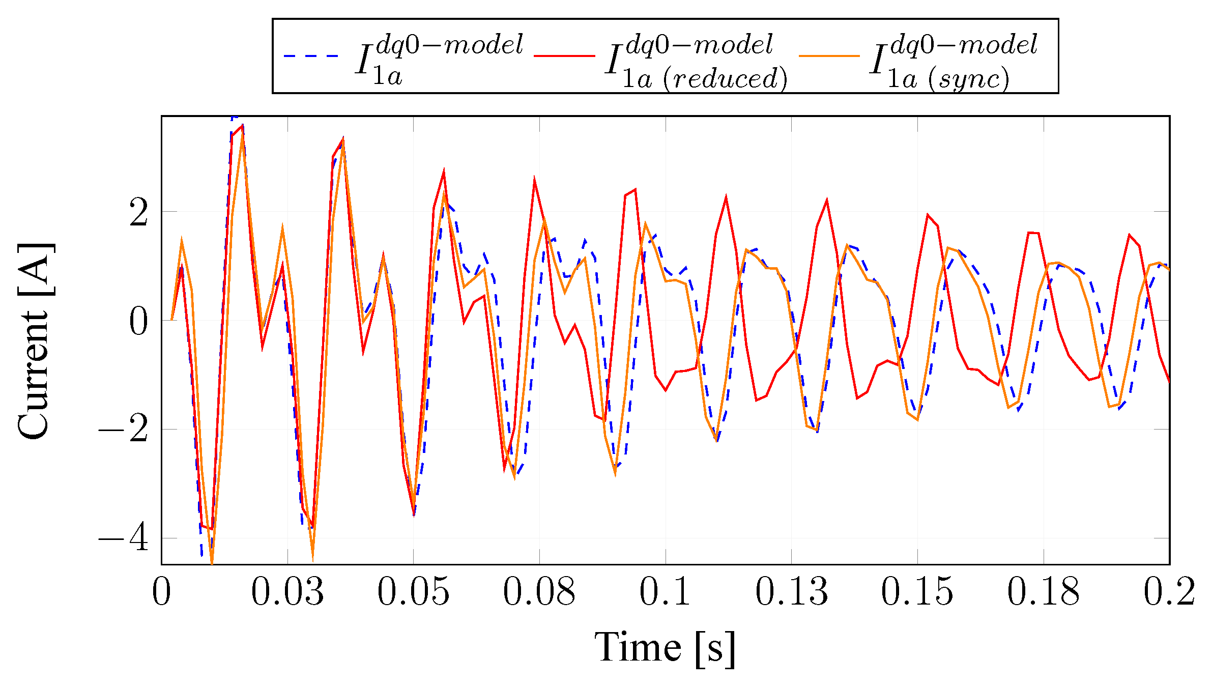
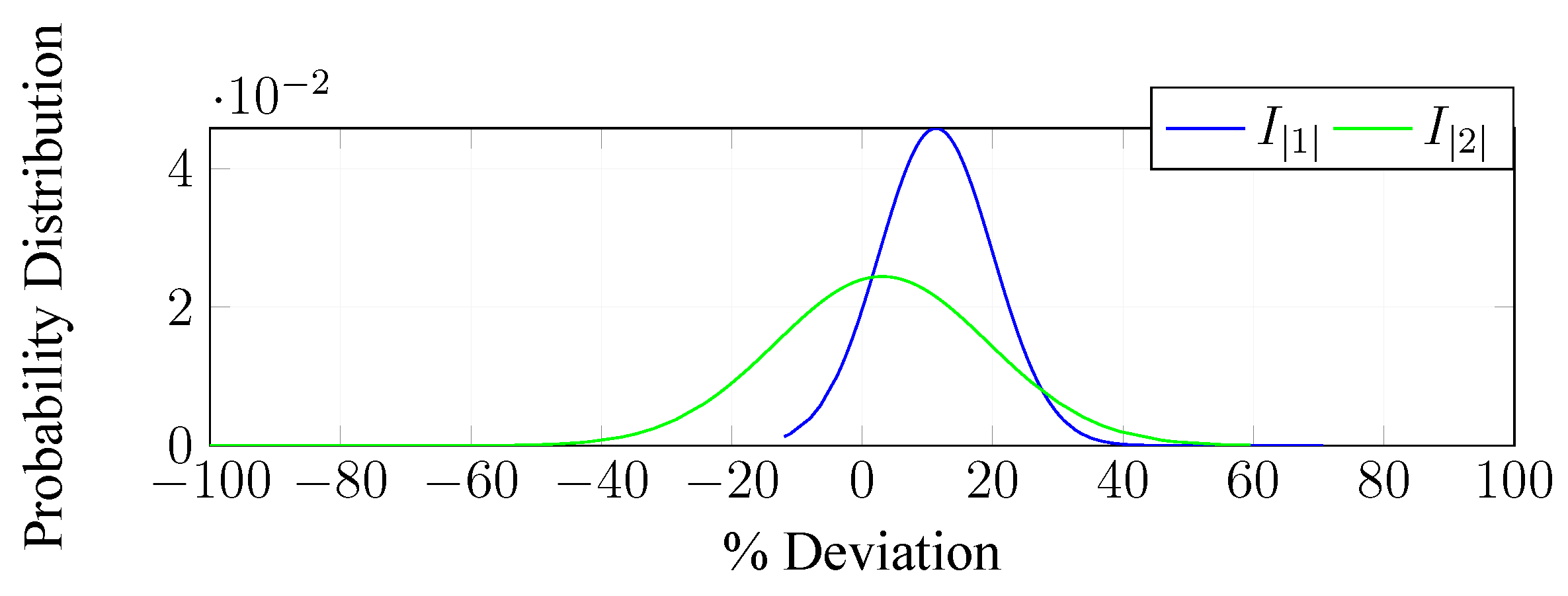
2.3. Component Selection for Reduced Order Model

For control purposes, it is convenient to develop a reduced order representation of the BDFIM with a single $dq$-rotor pair. Truncating the $dq0$-model will result in a poor representation of the original model. Due to the system not being time invariant in nature, reduction techniques for linear time-invariant (LTI) systems such as balanced truncation and optimal Hankel-norm approximation are not suitable for transient analysis [11]. Since the system is dependent on rotational speed, ${\omega }_r$, it can be called a linear parameter-varying system (LPV), for which generalizations of the Hankel-norm or balanced truncation techniques exist as well. However, for the physical interpretation of the machine to be maintained, techniques such as balanced truncation have to be applied to each component individually. For instance, the stator is already reduced, and as such, the technique should only be applied to the rotor. Therefore, it is desired to reduce the states of the rotor currents represented in Equation (17) as

$$\begin{array}{cc}\hfill \frac{d{i}_r}{dt}& =-\left[\begin{array}{c}{\left[{\mathit{M}}^{dq}\right]}_r^{-1}{R}_r+{\omega }_r{\left[{\mathit{M}}^{\mathit{dq}}\right]}_{sr}^{-1}{Q}_{sr}\end{array}\right]i_r+u,\hfill \end{array}$$

(19)

where the external stator currents and input voltage are represented by u. When applying the suitable reduction techniques, it becomes clear that it can be difficult to represent the balanced system in terms of mutual inductance, resistance, and the Q terms. As such, the designer loses insight into the physical interpretation of the component matrices. Accordingly, a method of reduction using an equivalent circuit mapping was proposed in [11]. The method is considered to be a good approximation for various rotor types; however, in [11], it was only applied to nested-loop-type rotors. In order to reduce the rotor states to two, a state order was chosen such as to order its eigenvalues in decreasing order from top left. To achieve this, the following steps were performed:

• A matrix $\mathit{T}$ which consists of eigenvectors of ${\mathit{M}}_r$ must be obtained and ordered such that its eigenvalues decrease from left to right.
• $\mathit{T}$ must be partitioned into two submatrices $\left[\begin{array}{cc}{\mathit{T}}_1& {\mathit{T}}_2\end{array}\right]$ where ${\mathit{T}}_1$ is two columns wide.
• Reduce the state order of the full-state $dq0$-reference frame BDFIM model by applying the nonsquare state transformation

  $$\begin{array}{c}\hfill i_{ReducedState}^{dq0}=\left[\begin{array}{cc}\mathit{I}& 0\\ 0& {\mathit{T}}_1^T\end{array}\right]i_{FullState}^{dq0},\end{array}$$

  (20)

  where $\mathit{I}\in {\mathbb{R}}^{6\times 6}$ is an identity matrix.

The transformation matrix ${\mathit{T}}_1$ will always be of the form:

$$\begin{array}{cc}\hfill {\mathit{T}}_1^T& =\left[\begin{array}{ccccccc}{\alpha }_1& 0& {\alpha }_2& 0& \cdots & {\alpha }_n& 0\\ 0& {\alpha }_1& 0& {\alpha }_2& \cdots & 0& {\alpha }_n\end{array}\right]\hfill \end{array}$$

(21)

From this, it is clear that the resulting reduced-state rotor matrix is an equivalently scaled representation of the original matrix. However, by careful selection of its eigenvalues, it can be reduced to retain as much of the original characteristics as possible. After the transformation has been applied, the final reduced order model can be shown to be:

$$\begin{array}{cc}\hfill \frac{d}{dt}\left[\begin{array}{c}{i}_s\\ {\tilde{i}}_{r1}\end{array}\right]=& \left[\begin{array}{cc}{M}_s& {\tilde{M}}_{sr1}\\ {\tilde{M}}_{sr1}^T& {\tilde{M}}_{r1}\end{array}\right]\hfill \\ \hfill & -\left[\begin{array}{cc}{R}_s& 0\\ 0& {\tilde{R}}_{r1}\end{array}\right]\left[\begin{array}{cc}{Q}_s& {\tilde{Q}}_{sr1}\\ 0& 0\end{array}\right]\left[\begin{array}{c}{i}_s\\ \widetilde{i_{r1}}\end{array}\right]+\left[\begin{array}{c}{v}_s\\ 0\end{array}\right]\hfill \end{array}$$

(22)

where the reduced order matrices are overset by tilde ($\tilde{}$).

2.4. Transformation into the Synchronous Space

The synchronous reference frame allows for numerous simplifications, greatly reducing the complexity of the resulting control system. It is convenient to derive an equivalent transformation from the rotor reference frame to the stator reference frame. In order to achieve this, a synchronous transformation matrix with reference to the primary stator windings is defined as,

$$\begin{array}{cc}\hfill {\mathit{T}}_{sync}& =\left[\begin{array}{ccc}cos(p_1{\theta }_r-{\omega }_{1}t)& sin(p_1{\theta }_r-{\omega }_{1}t)& 0\\ -sin(p_1{\theta }_r-{\omega }_{1}t)& cos(p_1{\theta }_r-{\omega }_{1}t)& 0\\ 0& 0& 1\end{array}\right],\hfill \end{array}$$

(23)

where ${\omega }_1$ is the stator 1 supply frequency. Stators 1 and 2 are aligned within the synchronous reference frame. This relies on the assumption that stators 1 and 2 are physically aligned, which may not always be an accurate assumption. However, the stators were aligned in this implementation. Applying the transformation matrix (${\mathit{T}}_{sync}$) to the rotor reference frame model, the synchronous reference frame model is derived as,

$$\begin{array}{cc}{\displaystyle \frac{d}{dt}}\left[\begin{array}{c}{i}_{s1}^{dq0}\\ i_{s2}^{dq0}\\ i_r^{dqr}\end{array}\right]\hfill & ={\mathit{M}}_{sync}^{-1}\left[\begin{array}{c}-{\mathit{R}}_{sync}-{\mathit{Q}}_{sync}\end{array}\right]\left[\begin{array}{c}{i}_{s1}^{dq0}\\ i_{s2}^{dq0}\\ i_r^{dqr}\end{array}\right]\hfill \\ & +{\mathit{M}}_{sync}^{-1}\left[\begin{array}{c}{v}_{s1}^{dq0}\\ v_{s2}^{dq0}\end{array}\right]\hfill \\ \hfill \end{array}$$

(24)

$$\begin{array}{cc}\hfill {\displaystyle \frac{d{\omega }_r}{dt}}=& {\displaystyle \frac{1}{2J}}{\left[\begin{array}{c}{i}_{s1}^{dq0}\\ i_{s2}^{dq0}\\ i_r^{dqr}\end{array}\right]}^T{\mathit{S}}_{sync}\left[\begin{array}{c}{i}_{s1}^{dq0}\\ i_{s2}^{dq0}\\ i_r^{dqr}\end{array}\right]-{\displaystyle \frac{T_l}{J}},\hfill \end{array}$$

(25)

where the equivalent torque and submatrices used for the derivation can be found in Appendix A.3.

Figure 5 shows a comparison of the reduced models, that is, the full 12-state model in the rotor reference frame, reduced 8-state rotor reference frame model, and equivalent 8-state synchronous frame model. It can be seen that all three simulations show responses in similar magnitude and period, with a slight phase offset.

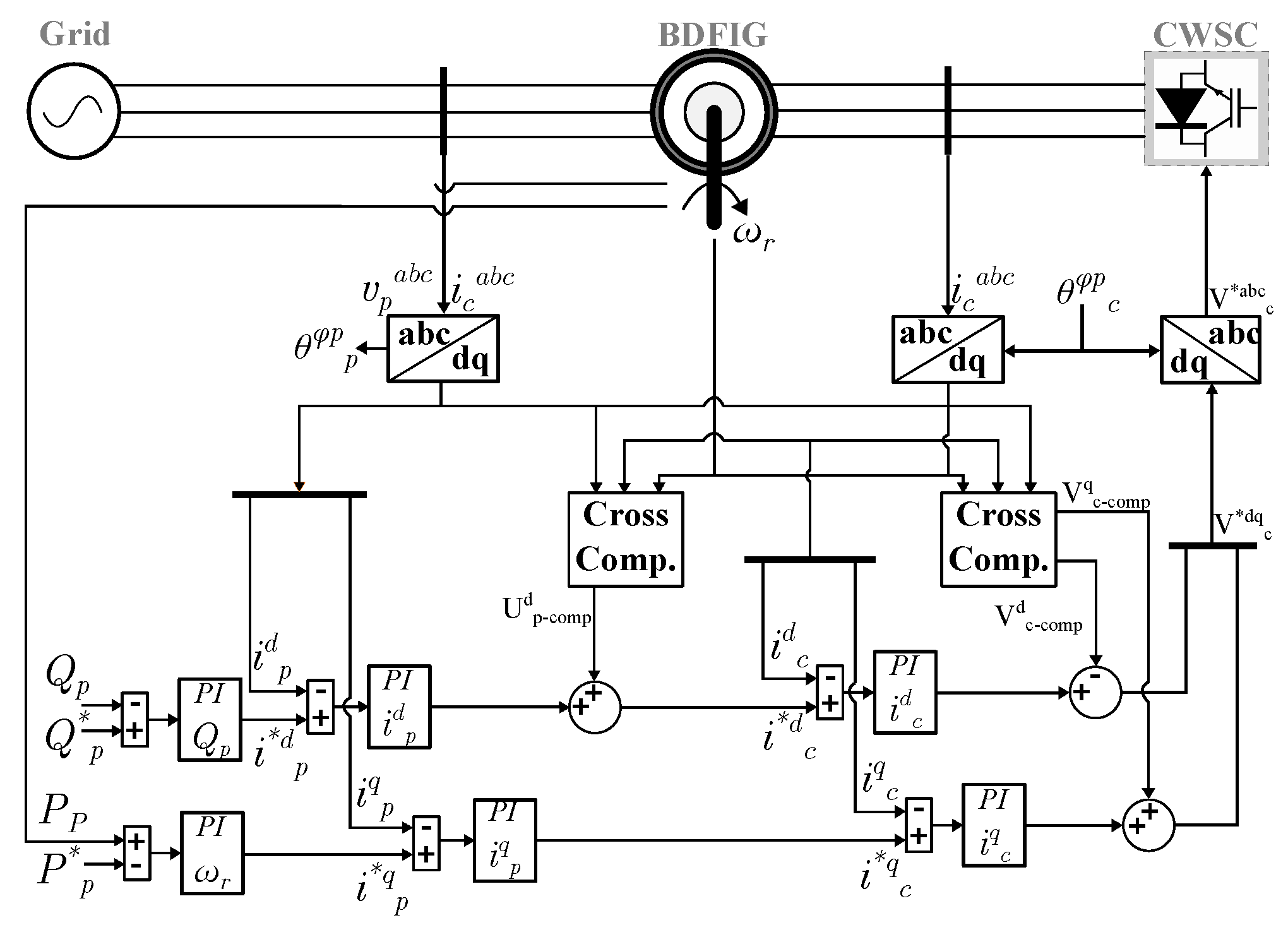
3. Control Winding Controller

The fundamental target of the control winding controller is to control the BDFIM’s active and reactive power. For torque and speed control, further derivations can follow based upon this fundamental. From Equation (24), the real and reactive power of the power winding in the rotating stator reference frame is defined as,

$$\begin{array}{c}\hfill P_{s1}=\frac{3}{2}{v}_{s1}^d{i}_{s1}^d+v_{s1}^q{i}_{s1}^q,Q_{s1}=\frac{3}{2}{v}_{s1}^q{i}_{s1}^d-i_{s1}^q{v}_{s1}^d.\end{array}$$

(26)

If the stationary reference frame is aligned with the d-axis of the stator power winding’s flux vector, ${\varphi }_s^d$, then the power equations simplify to [23,24],

$$\begin{array}{c}\hfill P_{s1}=\frac{3}{2}{v}_{s1}^q{i}_{s1}^q,Q_{s1}=\frac{3}{2}{v}_{s1}^q{i}_{s1}^d.\end{array}$$

(27)

The control winding’s voltage command signals can be expressed as

$$\begin{array}{cc}\hfill v_{s2}^{d*}& =R_{s2}{i}_{s2}^d+\frac{d}{dt}(-d_1{\varphi }_{s1}^d+d_2{\varphi }_r^d+d_3{i}_{s2}^d)-v_{s2-comp}^d\hfill \\ \hfill v_{s2}^{q*}& =R_{s2}{i}_{s2}^q+\frac{d}{dt}(d_2{\varphi }_r^q+d_3{i}_{s2}^q)+v_{s2-comp}^q,\hfill \end{array}$$

(28)

where

$$\begin{array}{cc}\hfill v_{s2-comp}^d& ={\omega }_{s2}(d_2{\varphi }_r^q+d_3{i}_{s2}^q)\hfill \\ \hfill v_{s2-comp}^q& ={\omega }_{s2}(-d_1{\varphi }_{s1}^d+d_2{\varphi }_r^d+d_3{i}_{s2}^d)\hfill \\ \hfill {\varphi }_{s2}^{dq}& =-d_1{\varphi }_{s1}^{dq}+d_2{\varphi }_r^{dq}+d_3{i}_{s2}^{dq},\hfill \\ \hfill d_1& =\frac{L_{ms1}{L}_{m\left(s2\right)}}{L_r{L}_{s\left(s1\right)}-L_{m\left(s1\right)}^2}\hfill \\ \hfill d_2& =\frac{L_{s\left(s1\right)}{L}_{m\left(s2\right)}}{L_r{L}_{s\left(s1\right)}-L_{m\left(s1\right)}^2}\hfill \\ \hfill d_3& =L_{s\left(s2\right)}-\frac{L_{s\left(s1\right)}{L}_{m\left(s2\right)}^2}{L_r{L}_{s\left(s1\right)}-L_{m\left(s1\right)}^2}.\hfill \end{array}$$

The dynamic disturbances caused by the rotor flux and the power winding are considered negligible in steady state and therefore, they are omitted from the inner-loop transfer function from here onwards. It can be shown that the transfer function for the plant can be approximated as,

$$\begin{array}{cc}\hfill H_{i\left(s2\right)}\left(s\right)& =\frac{i_{s2}^{dq}}{v_{s2}^{dq}}=\frac{\frac{1}{R_{s2}}}{1+\frac{d_3}{R_{s2}}s}.\hfill \end{array}$$

(29)

Recall that the $dq$-axis is aligned with flux vector ${\varphi }_{s1}^d$ and assuming that $R_{s1}{i}_{s1}<<j{\omega }_{s1}{\varphi }_{s1}$, the power winding’s flux can be approximated as

$$\begin{array}{c}\hfill {\varphi }_{s1}^d\approx \frac{v_{s1}^q}{{\omega }_{s1}}.\end{array}$$

(30)

The rotor flux can be estimated as,

$$\begin{array}{cc}\hfill {\varphi }_r& =\frac{L_{m\left(s1\right)}^2-L_r{L}_{s\left(s1\right)}}{L_{m\left(s1\right)}}{i}_{s1}+L_{m\left(s2\right)}{i}_{s2}+\frac{L_r}{L_{ms1}}{\varphi }_{s1}\hfill \end{array}$$

(31)

By substituting the rotor flux and rotor current into the rotor voltage equation and regarding the disturbances caused by the dynamic current changes to be negligible, the relationship between the power and control winding currents is given by,

$$\begin{array}{cc}\hfill i_{s2}=& \left[\frac{L_r{L}_{s\left(s1\right)}}{L_{m\left(s2\right)}{L}_{m\left(s1\right)}}-\frac{L_{m\left(s1\right)}}{L_{m\left(s2\right)}}-j\frac{L_{s\left(s1\right)}{R}_r}{{\omega }_{r\left(s1\right)}{L}_{m\left(s2\right)}{L}_{m\left(s1\right)}}\right]i_{s1}\hfill \\ \hfill +& \left[-\frac{L_r}{L_{m\left(s2\right)}{L}_{ms1}}+j\frac{R_r}{{\omega }_{r\left(s1\right)}{L}_{m\left(s2\right)}{L}_{m\left(s1\right)}}\right]{\varphi }_{s1}\hfill \end{array}$$

(32)

Note that the rotor-to-power-winding slip speed only becomes small enough to have a significant influence at a maximum rotor speed of four times the natural operating speed.

Therefore, for machines with poles in the power winding less than the amount of poles in the control winding (to ensure that the rotor-to-power-winding slip only becomes considerable at twice the natural operating speed), the imaginary terms in Equation (32) can be regarded as negligible. Additionally, due to the $dq$-axis alignment, the quadrature reference flux is zero and ${\varphi }_{s1}^d$ remains near constant. This results in the complete removal of cross-compensation between the winding currents, for the power winding control loop. However, there is still flux compensation ($U_{s1-comp}^{dq}$) to be added to the direct current control loop, that is,

$$\begin{array}{cc}\hfill i_{s2}^d& \approx \frac{L_r{L}_{s\left(s1\right)}-L_{m\left(s1\right)}^2}{L_{m\left(s2\right)}{L}_{m\left(s1\right)}}{i}_{s1}^d-\underset{U_{s1-comp}^{dq}}{\underbrace{\frac{L_r}{L_{m\left(s2\right)}{L}_{m\left(s1\right)}}{\varphi }_{s1}}}\hfill \\ \hfill i_{s2}^q& \approx \frac{L_r{L}_{s\left(s1\right)}-L_{m\left(s1\right)}^2}{L_{m\left(s2\right)}{L}_{m\left(s1\right)}}{i}_{s1}^q.\hfill \end{array}$$

(33)

The resulting transfer function used for PI control parameter design is approximated as,

$$\begin{array}{cc}\hfill H_{i\left(s1\right)}\left(s\right)& =\frac{i_{s1}^{dq}}{i_{s2}^{dq}}\approx \frac{L_{m\left(s2\right)}{L}_{m\left(s1\right)}}{L_r{L}_{s\left(s1\right)}-L_{m\left(s1\right)}^2}\hfill \end{array}$$

(34)

Due to the linearity of the zero-order function above, it is recommended to remove the PI control for the power winding loop, since it can be compensated for by the PI controllers upstream, should the objective of the control be not to directly control the power winding currents.

Similar to [25], the torque and rotor speed transfer functions can be obtained to be

$$\begin{array}{cc}\hfill \frac{T_e}{i_{s1}^q}& \approx \frac{3}{2}(p_{s1}+p_{s2}){\varphi }_{s1}^d\hfill \end{array}$$

(35)

In order to control the reactive power in the power winding, it is necessary to determine the reference reactive power as a function of the reference current $i_{s1}^d$. By substituting the estimated power winding’s flux into the reactive power Equation (27), the transfer function for the control of reactive power is

$$\begin{array}{c}\hfill \frac{Q_{s1}}{i_{s1}^d}=\frac{3}{2}{\omega }_{s1}{\varphi }_{s1}^d\end{array}$$

(36)

The schematic of the machine with the developed controller is shown in Figure 6.

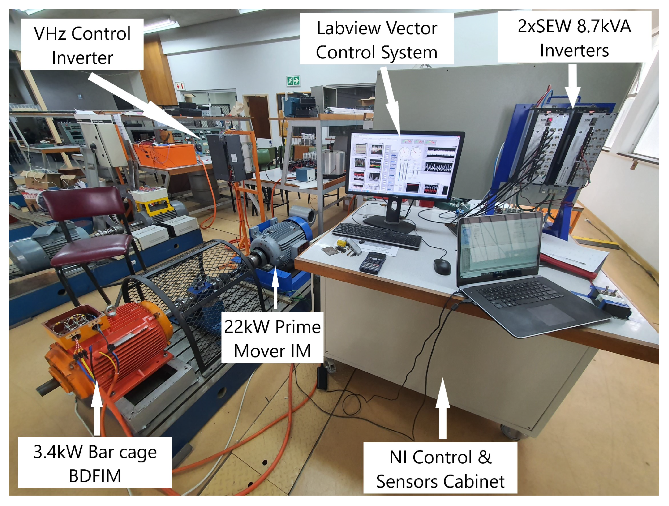
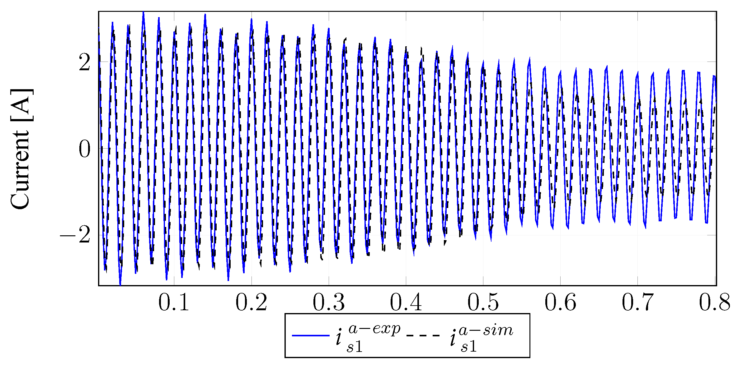
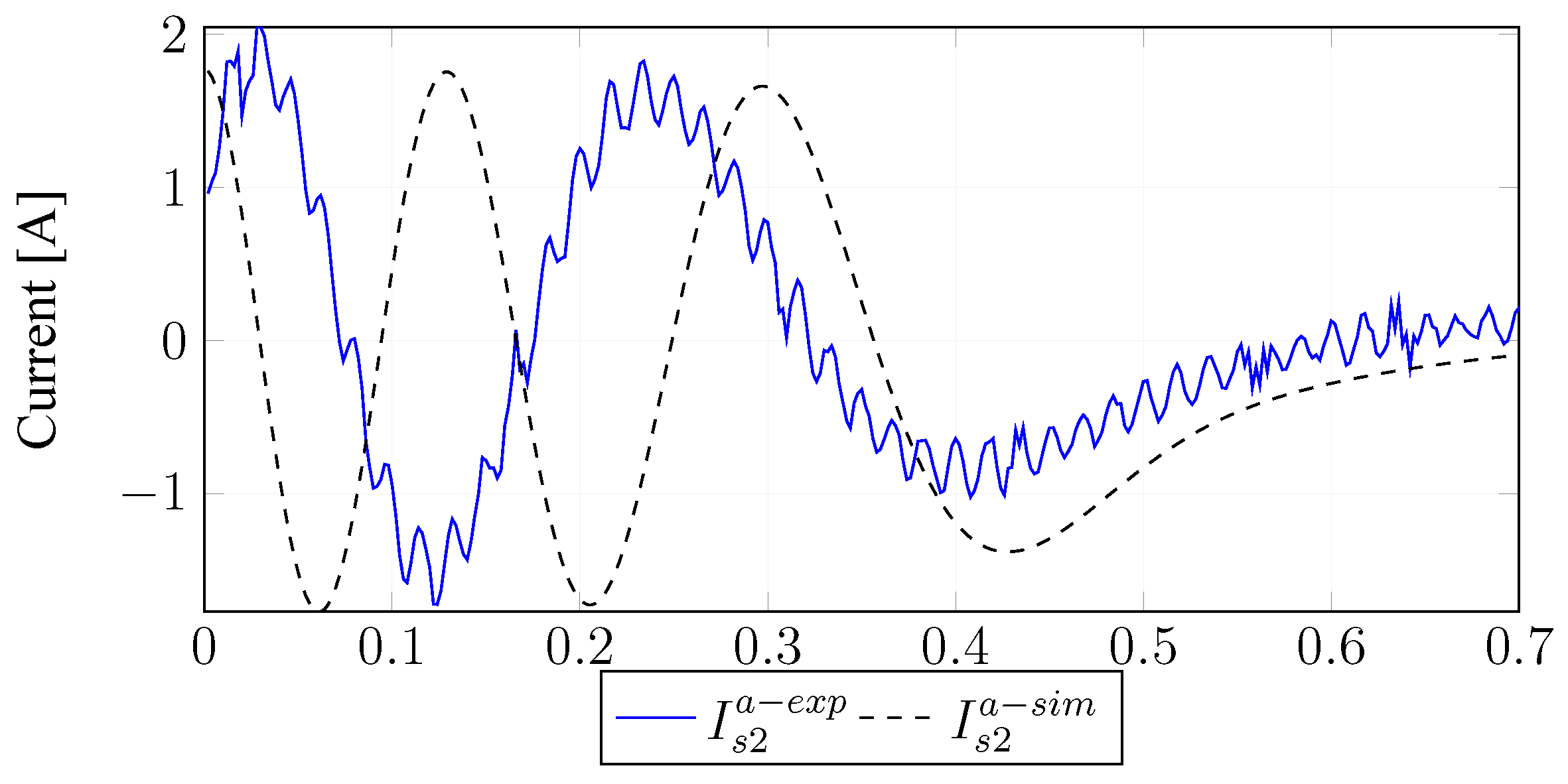
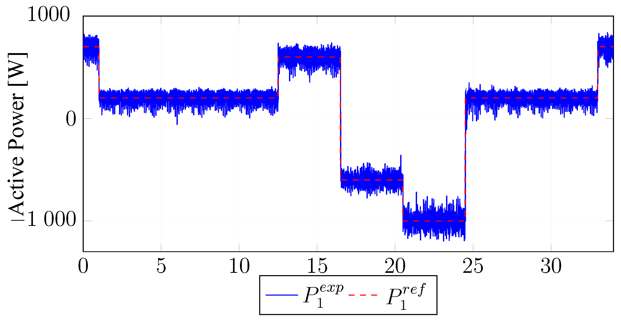
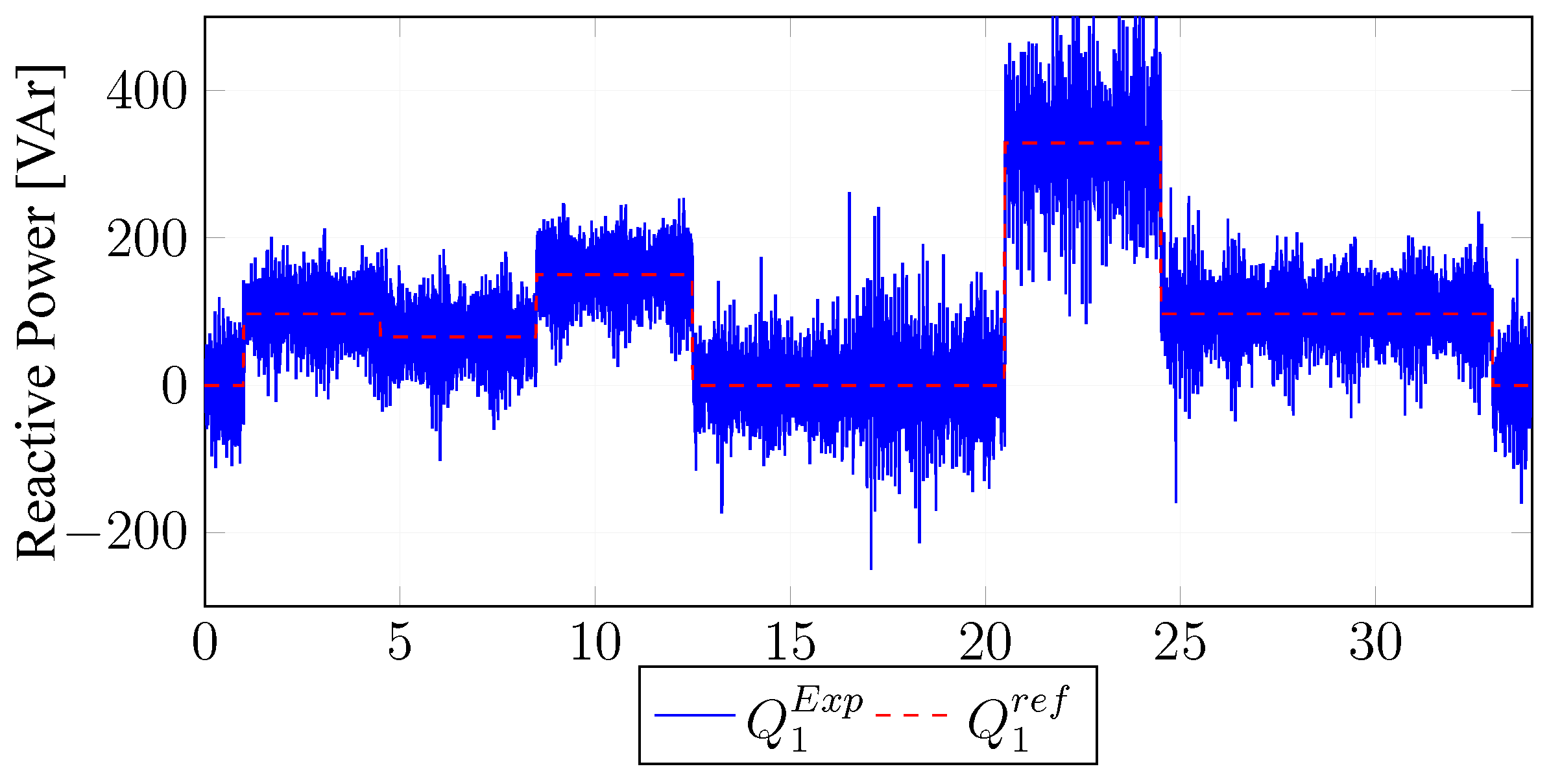
4. Experimental Test Results

An experimental setup was used to verify the theoretical derivations. The aim was to validate the simplified model in conjunction with the developed controller.

As shown in Figure 7, the BDFIG test bench consisted of a custom designed prototype three-phase 3.4 kW cage+NL BDFIG directly coupled to a 22 kW induction motor. The specifications of the BDFIG are given in the appendix. The test bench setup allowed for both motoring and generation modes investigations. The control algorithm was implemented in a National Instrument (NI) PXIe-8115 embedded real-time controller. The proposed control strategies designed in Simulink were implemented for the experimental test bench using LabVIEW. Additionally, the test bench also included two NI 7841R FPGA expansion modules that allowed for both input and output signals to or from the PXIe-8115 controller. Furthermore, the back-to-back converter consisted of two 8.7 kVA custom-modified with a switching frequency of 5 kHz from commercially available SEW power converters. For the purpose of this setup only the control winding’s side controller was investigated and a stable grid side controller was assumed. The measurements of the three-phase voltages were obtained using LEM LV25-P sensors and that of the three-phase currents were measured using LA55-P sensors. A GI341 BAUMER incremental encoder, mounted on the rotor shaft was used to measure the rotor speed and angle.

The deviation of the measured results of the stator’s currents is shown in Figure 8. In the figure, the distribution of the simulated versus actual measurements over the subsynchronous speed range of the motor is shown. A mean deviation of $11.32$% to the estimated readings for the stator’s power winding ($I_{\left|1\right|}$) and $3.06$% for the stator’s control windings ($I_{\left|2\right|}$) is observed. Additionally, the standard deviation for the power winding currents was determined to be $8.71$ and $16.34$ for the control winding currents. This indicated that although the model current estimates for the power winding currents were slightly offset from the real values, the surety of the estimates were more reliable than for the control windings.

Due to the physical limitations of accessibility to the rotor, measurements of the rotor bar’s currents were impractical, and thus the induced currents into the control winding were used for comparison, essentially visualizing the machine as a black box with the power winding as input and control winding currents as output. At first, the BDFIM was investigated in motoring mode whereby the control winding was short-circuited. In Figure 9, a comparison between the simulated and experimental cage+NL BDFIM motor power winding stator phase a current is shown. It is observed that the currents are oscillating as expected at the grid frequency of 50 Hz. The currents start out with very similar amplitudes of ≈2.5 A and soon after, the simulated currents reduce to a peak amplitude of $1.2$ A compared to the peak of $1.7$ A in the primary stator.

The control windings induced phase a currents are shown in Figure 10. Both simulated and experimental results show similar current peaks and periods. However, a phase shift is seen, which is likely due to the difference in rotor speed causing a drift in angular position during startup.

In Figure 11 and Figure 12, respectively, the controlled active and reactive power of the machine while transitioning between generation and motoring modes can be observed. It can be observed that the controller sufficiently tracks the reference powers. Through physical tests, it was found that the observable noise level in the figures is due to sensor noise that was caused by the modified inverter. In the future, a converter with less noise, operating at a higher frequency, can be used to reduce the noise. However, the noise does not affect the conclusion on the performance of the control method.

5. Conclusions

In this paper, it was shown that the method presented in [11] can be used to model a cage+NL rotor BDFIM for control purposes. In [11], a method was presented for the modeling of BDFIM and in this work, that method was validated through simulation and practical measurements for a new rotor (cage+NL rotor) BDFIM. A full-state model of a cage+NL rotor BDFIM was presented. A model reduction technique was utilized in order to develop a portable model that can be used in the development of a vector control algorithm for the cage+NL rotor BDFIM. To ensure accurate simulation results, the full expanded BDFIM model (23-state model for the BDFIM under consideration) was compared to the reduced model and to practical measurements. Both the full-state and reduced-order models showed satisfactory comparison to that of the physical machine during free acceleration. The controllers demonstrated good stability and accurate response times, indicating that the vector control parameters were within reasonable tolerances for the PI controllers to be stable. Different modes of operation were analyzed, whereby the machine response under synchronous, sub- and supersynchronous speeds was shown.

References

1. Brune, C.; Spee, R.; Wallace, A.K. Experimental evaluation of a variable-speed, doubly-fed wind-power generation system. IEEE Trans. Ind. Appl. 1993, 30, 480–487. [Google Scholar] [CrossRef]
2. Artigao, E.; Sapena-Bano, A.; Honrubia-Escribano, A.; Martinez-Roman, J.; Puche-Panadero, R.; Gómez-Lázaro, E. Long-Term Operational Data Analysis of an In-Service Wind Turbine DFIG. IEEE Access 2019, 7, 17896–17906. [Google Scholar] [CrossRef]
3. Löhdefink, P.; Dietz, A.; Möckel, A. Direct drive concept for heavy-duty traction applications with the brushless doubly-fed induction machine. In Proceedings of the 2018 13th International Conference on Ecological Vehicles and Renewable Energies (EVER), Monte Carlo, Monaco, 10–12 April 2018; pp. 1–6. [Google Scholar] [CrossRef]
4. Gabriel, R.; Leonhard, W.; Nordby, C.J. Field-oriented control of a standard ac motor using microprocessors. IEEE Trans. Ind. Appl. 1980, 1, 186–192. [Google Scholar] [CrossRef]
5. Spee, R.; Wallace, A.K.; Lauw, H.K. Performance simulation of brushless doubly-fed adjustable speed drives. In Proceedings of the Conference Record of the IEEE Industry Applications Society Annual Meeting, San Diego, CA, USA, 1–5 October 1989; Volume 1, pp. 738–743. [Google Scholar] [CrossRef]
6. Wallace, A.K.; Spee, R.; Lauw, H.K. Dynamic modeling of brushless doubly-fed machines. In Proceedings of the Conference Record of the IEEE Industry Applications Society Annual Meeting, San Diego, CA, USA, 1–5 October 1989; Volume 1, pp. 329–334. [Google Scholar] [CrossRef]
7. Boger, M.S.; Wallace, A.K.; Spee, R.; Li, R. General pole number model of the brushless doubly-fed machine. IEEE Trans. Ind. Appl. 1995, 31, 1022–1028. [Google Scholar] [CrossRef]
8. Li, R.; Wallace, A.; Spee, R. Dynamic simulation of brushless doubly-fed machines. IEEE Trans. Energy Convers. 1991, 6, 445–452. [Google Scholar] [CrossRef]
9. Li, R.; Wallace, A.; Spee, R.; Wang, Y. Two-axis model development of cage-rotor brushless doubly-fed machines. IEEE Trans. Energy Convers. 1991, 6, 453–460. [Google Scholar] [CrossRef]
10. Boger, M.S. Aspects of Brushless Doubly-Fed Induction Machines. Ph.D. Thesis, St. John’s College, University of Cambridge, Cambridge, UK, 2015. [Google Scholar] [CrossRef]
11. Roberts, P.C. Study of Brushless Doubly-Fed (Induction) Machines: Contributions in Machine Analysis, Design and Control. Ph.D. Thesis, St. John’s College, University of Cambridge, Cambridge, UK, 2015. [Google Scholar] [CrossRef]
12. Zhou, D.; Spee, R.; Alexander, G.C. Experimental evaluation of a rotor flux oriented control algorithm for brushless doubly-fed machines. IEEE Trans. Power Electron. 1997, 12, 72–78. [Google Scholar] [CrossRef]
13. Munoz, A.R.; Lipo, T.A. Complex vector model of the squirrel-cage induction machine including instantaneous rotor bar currents. IEEE Trans. Ind. Appl. 1999, 35, 1332–1340. [Google Scholar] [CrossRef] [Green Version]
14. Munoz, A.R.; Lipo, T.A. Dual stator winding induction machine drive. IEEE Trans. Ind. Appl. 2000, 36, 1369–1379. [Google Scholar] [CrossRef]
15. Barati, F.; Oraee, H.; Abdi, E.; Shao, S.; McMahon, R. The Brushless Doubly-Fed Machine Vector Model in the rotor flux oriented reference frame. In Proceedings of the 2008 34th Annual Conference of IEEE Industrial Electronics Society, Orlando, FL, USA, 10–13 November 2008; pp. 1415–1420. [Google Scholar] [CrossRef]
16. Rodriguez, M. Unified reference frame dq model of the brushless doubly fed machine. IEE Proc.-Electr. Power Appl. 2006, 153, 726–734. [Google Scholar]
17. Poza, J.; Oyarbide, E.; Sarasola, I.; Rodriguez, M. Vector control design and experimental evaluation for the brushless doubly fed machine. IET Electr. Power Appl. 2009, 3, 247–256. [Google Scholar] [CrossRef]
18. Barati, F.; Oraee, H.; Abdi, E.; McMahon, R. Derivation of a vector model for a Brushless Doubly-Fed Machine with multiple loops per nest. In Proceedings of the 2008 IEEE International Symposium on Industrial Electronics, Vigo, Spain, 4–7 June 2008; pp. 606–611. [Google Scholar] [CrossRef]
19. Barati, F.; Oraee, H. Vector model utilization for nested-loop rotor Brushless Doubly-Fed Machine analysis, control and simulation. In Proceedings of the 2010 1st Power Electronic & Drive Systems & Technologies, Tehran, Iran, 17–18 February 2010; pp. 295–301. [Google Scholar] [CrossRef]
20. Barati, F.; Shao, S.; Abdi, E.; Oraee, H.; McMahon, R. Synchronous operation control of the Brushless Doubly-Fed Machine. In Proceedings of the 2010 IEEE International Symposium on Industrial Electronics, Bari, Italy, 4–7 July 2010; pp. 1510–1516. [Google Scholar] [CrossRef]
21. Barati, F.; McMahon, R.; Shao, S.; Abdi, E.; Oraee, H. Generalized vector control for brushless doubly fed machines with nested-loop rotor. IEEE Trans. Ind. Electron. 2013, 60, 2477–2485. [Google Scholar] [CrossRef]
22. Olubamiwa, O.; Gule, N.; Kamper, M. Coupled circuit analysis of the brushlessdoubly fed machine using the windingfunction theory. IET Electr. Power Appl. 2020, 14, 1558–1569. [Google Scholar] [CrossRef]
23. Abu-Rub, H.; Iqbal, A.; Guzinski, J. High Performance Control of AC Drives with MATLAB/Simulink Models; John Wiley & Sons: Hoboken, NJ, USA, 2012. [Google Scholar]
24. Lobo, F.J.P. Modélisation, Conception et Commande d’Une Machine Asynchrone Sans Balais Doublement Alimentée Pour la Génération à Vitesse Variable. Ph.D. Thesis, Institut National Polytechnique de Grenoble-INPG, Grenoble, France, 2003. [Google Scholar]
25. Poza, J.; Oyarbide, E.; Roye, D. New vector control algorithm for brushless doubly-fed machines. In Proceedings of the IEEE 2002 28th Annual Conference of the Industrial Electronics Society IECON 02, Sevilla, Spain, 5–8 November 2002; Volume 2, pp. 1138–1143. [Google Scholar] [CrossRef]
Figure 1. Bushless doubly fed induction machine (BDFIM) implementation as a wind turbine.
Energies 15 05238 g001
Figure 2. Cage+NL rotor structure for a brushless doubly fed induction machine [22].
Energies 15 05238 g002
Figure 3. BDFIM cage+NL rotor equivalent circuit [22].
Energies 15 05238 g003
Figure 4. BDFIM full-state coupled circuit model’s middle loop currents compared with the d q 0 equivalent model during startup with zero initial current and natural speed.
Energies 15 05238 g004
Figure 5. Simulation results of the phase a current response of the BDFIM’s d q 0 -rotor-reference frame model (12-state model) compared to the d q 0 -reduced model (8-state model) and the d q 0 synchronous model (8-state model).
Energies 15 05238 g005
Figure 6. Control winding’s side controller with active and reactive power regulation.
Energies 15 05238 g006
Figure 7. BDFIG test bench setup showing the BDFIG, the induction motor, the inverter, and the control system.
Energies 15 05238 g007
Figure 8. Spread of deviation of simulated currents compared to measured currents.
Energies 15 05238 g008
Figure 9. BDFIM power winding currents during startup.
Energies 15 05238 g009
Figure 10. BDFIM measured and simulated control winding currents during startup.
Energies 15 05238 g010
Figure 11. Measured BDFIM generator’s active power.
Energies 15 05238 g011
Figure 12. Measured BDFIM generator’s reactive power.
Energies 15 05238 g012
Publisher’s Note: MDPI stays neutral with regard to jurisdictional claims in published maps and institutional affiliations.