Adaptive Sliding-Mode Control for Electric Spring in Microgrids with Distributed Renewable Energy

Abstract

Electric springs (ESs) are novel electric-power devices that alleviate power-quality problems such as voltage fluctuations induced by grid access to renewable energy resources. However, with the continuous increase of uncertain factors such as parameter perturbation and external disturbance, the environment becomes more complicated, so traditional linear controllers for ESs are finding it increasingly difficult to meet the control requirements due to narrow stability regions, low precision, and poor robustness. To overcome this problem, we propose herein a control method that combines adaptive control and sliding-mode control and apply it to ESs. First, an inexact model of the ES system was established and analyzed. Next, an ES control system was designed based on adaptive sliding-mode control, and then the asymptotic stability of the closed-loop system is proven. Finally, the proposed control system was verified through a MATLAB simulation. The results show that adaptive sliding-mode control not only ensures the voltage stability of critical loads in the microgrid but also resists the influence of parameter perturbation and external disturbances, leading to better steady-state and dynamic performance than a linear controller.

1. Introduction

In recent years, with the growing problem of global environmental pollution and energy shortages, renewable energy sources (RESs) represented by wind and solar energy have developed rapidly [1]. The continuous access of distributed RESs has led to the low-voltage network and microgrid developing toward a green and sustainable design [2,3]. However, the inherent intermittence and uncertainty of RESs make it difficult to accurately predict power generation [4], which increases the difficulty for utility companies to maintain the instantaneous power balance between supply and demand and exacerbates problems such as voltage fluctuations and voltage out-of-limit in the distribution network or microgrid. Moreover, the increasing permeability of RESs makes the problem of voltage fluctuation more and more prominent [5,6].

To deal with voltage fluctuations within distribution networks or microgrids, the demand side management method [7,8,9,10] is adopted to directly manage the load on the user side, allowing the load demand to be matched with the power generation and thereby alleviating voltage fluctuations. Although these methods have their own advantages for suppressing voltage fluctuation, they also come with inherent limitations. For example, real-time pricing [7] and day-ahead power-demand scheduling [8] cannot respond instantaneously to demand, direct load on/off control [9] sacrifices the comfort of power users, and energy storage systems [10] suffer from short lifespan, limited capacity, and large cost. Therefore, fast, convenient, and cost-effective demand response technology must be developed.

Inspired by mechanical springs, the Hui research group of the University of Hong Kong proposed the electric spring (ES) technology in 2012 [11], forming a new demand-side management method. ESs divide loads into critical loads (CLs) and noncritical loads (NCLs) according to the range of voltage fluctuations that they can withstand. CLs must be continuously supplied with a stable voltage. NCLs can withstand a wider range of voltage fluctuations, and their consumption can be modulated. For example, medical equipment that requires high-quality power should be considered a CL, whereas residential or shopping-mall heating and cooling loads can be considered an NCL. An ES and a NCL in series form a smart load. ESs adjust their own voltage output in real-time as a function of supply-side voltage fluctuations to control voltage variations in the NCL, so supply-side voltage fluctuations are transferred to the NCL, and the CL voltage remains stable.

Compared with traditional demand-side management methods, ESs have the advantages of smaller energy-storage requirements, lower cost (compared with energy-storage systems) [12], and better higher-quality power (compared with direct-load on-off control). After years of research, ESs are now available in several versions and are suitable for power-factor correction, harmonic suppression, frequency stabilization, and other tasks [13,14].

Several control schemes for ESs have been reported. Ref. [15] proposes radial chordal decomposition control to endow ESs with simultaneous power-factor correction and voltage regulation. The “δ control scheme” based on a proportional resonant (PR) controller was proposed in Ref. [16] and serves to simultaneously regulate voltage and suppress harmonics. This scheme is more accurate than radial chordal decomposition but requires a communication network to transmit supply-side voltage information. Ref. [17] proposed three interior angle control principles for the ES, which were then analyzed and compared until, finally, presenting a generalized control structure suitable for implementing all these three angle control methods. Ref. [18] proposed a new control strategy based on a direct current control mode to improve the performances of ESs based on current–source inverters. In the present work, the active power and reactive power of ESs are decoupled by dq0 transformation to simultaneously implement the functions of harmonic suppression, voltage regulation, and power-factor correction.

Although these controls have different structures because they were designed to deal with different problems, they all use linear controllers (proportional integral (PI) controllers or PR controllers). Linear controllers are easy to implement, but it has the disadvantages of narrow stability range, poor robustness, and control effects that are easily affected by parameter perturbation and external disturbances. In addition, the parameter debugging of linear controllers is time-consuming and laborious. Given the increasing number of nonlinear loads and uncertain disturbances, linear controllers of ES systems no longer satisfy the control requirements [19]. To improve the control effect, many researchers have optimized the parameters of traditional linear controllers or have combined linear control with other methods. Ref. [20] proposed a control method that combines quasi-proportional resonance control and repetitive control. Compared with the traditional PR control, this method improves the steady-state accuracy and reduces the system harmonic. Ref. [21] first applies an improved particle swarm algorithm to calculate the initial parameters of the PI controller, and then adjusts the parameters of the PI controller in real time by using a fuzzy algorithm. The results show that this strategy improves the control accuracy of ES. To minimizing the CL voltage error, Ref. [22] uses a genetic algorithm to optimize the PI controller parameters. The simulation shows that optimizing the parameters improves the adaptability and robustness of the PI controller. However, Refs. [20,21,22] did not study the influence of parameter perturbation and external disturbance. Considering the switching of NCL during operation, Refs. [23,24] proposed a self-adaptive voltage control strategy. Ref. [23] adjusts the gain of the PI controller in real time according to the output current of ES, and Ref. [24] adjusts the fuzzy universe according to the input errors, to improve the PI controller parameters. These two strategies ensure the stability of CL voltage when NCL changes, but the variations of other parameters such as filter inductance and DC side voltage are not considered. These researchers have made linear controllers that are more robust and adaptable, and the control effect has been improved. However, these control methods still do not suffice to deal with the multivariable and strongly coupled nonlinear characteristics of ESs and do not overcome the influence of uncertain disturbances such as variations in system parameters and external disturbances. In contrast with PI or PR control, sliding-mode control (SMC) is a special type of nonlinear control whose main characteristic is the discontinuity of the control structure. The control system switches between different structures as a function of the current state of the controlled object, forcing the controlled object to follow a predetermined state trajectory. The SMC responds rapidly and is not affected by system parameter perturbations, external disturbances, etc. [25,26,27]. Given that the variable structure characteristics of sliding-mode control are similar to the switching characteristics of ES converters, we apply it to the control of ESs.

This paper introduces adaptive sliding-mode control (ASMC) as an ES control system to make ESs more robust against interference and optimize their dynamic and static performance. We start by analyzing the working principle of ESs and derive an inexact state equation that considers parameter perturbation and external disturbances. Next, we use an adaptive prediction to estimate the total uncertainty of the system and obtain the minimum switching gain that satisfies the system-stability requirements. On this basis, the ASMC method is designed by combining adaptive control and sliding-mode control, following which the stability of the method is demonstrated. Finally, the advantages of the proposed control strategy are revealed by MATLAB simulations.

2. Electric-Spring Structure and Model Analysis

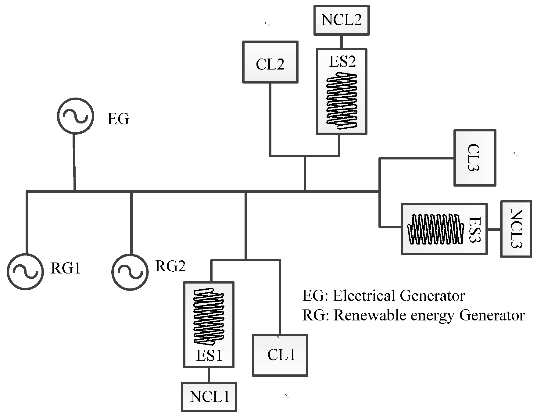
Figure 1 shows a simplified diagram of a microgrid with distributed generation, ESs, and renewable energy generators (RGs). Renewable sources can be wind energy, solar energy, tidal energy, etc. An electrical generator (EG) is a micro gas turbine or a diesel generator that offers adjustable power generation. EGs implement the power-generation plan made by microgrid operators based on the predictions of the power that can be generated by renewable sources. Accurate forecasting helps operators reduce the impact of the variability of renewable-source power on the microgrid, thereby improving the reliability of the microgrid. However, such power predictions are easily influenced by factors such as weather, temperature, and dust. Therefore, the intermittent uncertainty of renewable power sources inevitably leads to discrepancies between the predicted power and actual power, resulting in branch–voltage deviation from the target value. Therefore, ESs are required to allow active control and keep the CL voltage stable.

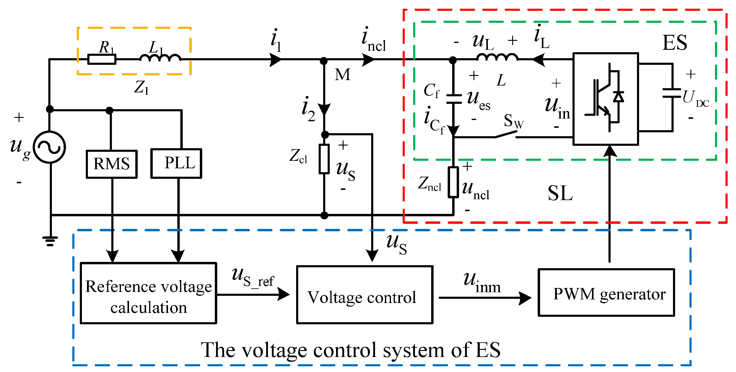
Figure 2 shows a typical circuit with a single ES, where $u_{\mathrm{g}}$ is the supply-side voltage, $u_{\mathrm{S}}$ is the CL voltage, Z₁ is the transmission-line impedance, and Z_cl and Z_ncl are the impedances of the CL and NCL, respectively. The ES is contained within the green dashed rectangle and is composed of a voltage–source inverter, a filter inductor, a filter capacitor, and an access switch S_W. When S_W is open, the ES has no effect and acts only as a capacitor. Smart loads and Z_cl are connected in parallel, and the assembly is connected to a point of common coupling. When $u_{\mathrm{g}}$ fluctuates, the ES adjusts its own output voltage, thereby adjusting the voltage across Z_ncl to make the NCL consume power adaptively. In addition, it also acts as a reactive power generator to regulate the reactive power of the system. These two aspects allow ESs to stabilize $u_{\mathrm{S}}$.

The blue dotted frame contains the ES control system, in which the module for calculating the reference voltage calculates the CL reference voltage u_{S_ref} from $u_{\mathrm{g}}$ and the system parameters. According to $u_{\mathrm{S}}$ and $u_{\mathrm{S}\_\mathrm{ref}}$, the voltage control module generates a pulse–width modulation wave to control the on-off inverter switch tube, thereby adjusting the output voltage of the ES to stabilize the root-mean-square (RMS) voltage of $u_{\mathrm{S}}$ at a preset value. According to $u_{\mathrm{g}}$, the ES works in one of three modes: inductive, resistive, and capacitive. When $u_{\mathrm{es}}=0$, ES works in resistive mode and does not exchange reactive power with the grid. The RMS of $u_{\mathrm{g}}$ at this point is denoted $U_{\mathrm{g}\_\mathrm{ref}}$. When the RMS of $u_{\mathrm{g}}$ exceeds $U_{\mathrm{g}\_\mathrm{ref}}$, the ES absorbs reactive power and works in inductive mode. If the RMS of $u_{\mathrm{g}}$ is less than $U_{\mathrm{g}\_\mathrm{ref}}$, the ES releases reactive power and works in capacitive mode.

By applying Kirchhoff’s law in Figure 2, we obtain

$$\begin{array}{c}{i}_{C_f}=i_{ncl}+i_L,\\ u_{es}=u_{in}-u_L.\end{array}$$

(1)

Taking $u_{\mathrm{es}}$ and its derivative as the state variables,

$$\begin{array}{c}{x}_1=u_{\mathrm{es}},\\ x_2={\dot{u}}_{\mathrm{es}},\end{array}$$

(2)

allows the system state equations to be derived from Figure 2:

$$\begin{array}{c}{\dot{x}}_1=x_2={\dot{u}}_{\mathrm{es}},\hfill \\ {\dot{x}}_2={\ddot{u}}_{\mathrm{es}}=\frac{u_{\mathrm{in}}}{L{C}_{\mathrm{f}}}-\frac{u_{\mathrm{es}}}{L{C}_{\mathrm{f}}}+\frac{{\dot{i}}_{\mathrm{ncl}}}{C_{\mathrm{f}}}.\hfill \end{array}$$

(3)

Considering the perturbation of a system parameter and an external disturbance, Equation (3) can be rewritten as

$$\begin{array}{c}{\dot{x}}_1={\dot{u}}_{\mathrm{es}},\hfill \\ {\dot{x}}_2={\ddot{u}}_{\mathrm{es}}=\left(\frac{1}{L{C}_{\mathrm{f}}}+\Delta a\right)\left(u_{\mathrm{in}}-u_{\mathrm{es}}\right)+\left(\frac{1}{C_{\mathrm{f}}}+\Delta b\right){\dot{i}}_{\mathrm{ncl}}+\Delta d,\hfill \end{array}$$

(4)

where $\Delta a$ and $\Delta b$ are the perturbations of $L{C}_{\mathrm{f}}$ and $C_{\mathrm{f}}$, respectively, and $\Delta d$ is an external disturbance such as the DC side voltage $U_{\mathrm{DC}}$ of the inverter fluctuations.

The total uncertainty of the system can be expressed as

$$\omega (t)=\Delta a\left(u_{\mathrm{in}}-u_{\mathrm{es}}\right)+\Delta b{\dot{i}}_{\mathrm{ncl}}+\Delta d.$$

(5)

Equation (4) can be simplified as

$$\begin{array}{c}{\dot{x}}_1={\dot{u}}_{\mathrm{es}},\hfill \\ {\dot{x}}_2=\frac{K_{\mathrm{PWM}}{u}_{\mathrm{inm}}}{L{C}_{\mathrm{f}}}-\frac{u_{\mathrm{es}}}{L{C}_{\mathrm{f}}}+\frac{{\dot{i}}_{\mathrm{ncl}}}{C_{\mathrm{f}}}+\omega (t),\hfill \end{array}$$

(6)

where $K_{\mathrm{PWM}}=U_{\mathrm{DC}}/U_{\mathrm{tri}}$ is the inverter gain, $U_{\mathrm{tri}}$ is the amplitude of the triangular carrier wave, and $u_{\mathrm{inm}}$ is the PWM modulation signal. Since the total uncertainty of the system is bounded, we assume $\rho >0$ is the (constant) upper bound, so $\left|\omega (t)\right|\le \rho$.

3. Electric Spring Adaptive Sliding-Mode Control

3.1. Design Principles of Adaptive Sliding-Mode Controller

Taking the deviation of $u_{\mathrm{S}}$ from $u_{\mathrm{S}\_\mathrm{ref}}$ and its time derivative as the new state variables,

$$\begin{array}{c}{x}_1=u_{\mathrm{S}}-u_{{\mathrm{S}}_{-}\mathrm{ref}},\\ x_2={\dot{u}}_{\mathrm{S}}-{\dot{u}}_{{\mathrm{S}}_{-}\mathrm{ref}},\end{array}$$

(7)

gives a new state equation for the ES of Figure 2 when combined with Equation (6):

$$\begin{array}{l}{\dot{x}}_1=\dot{e}={\dot{u}}_{\mathrm{S}}-{\dot{u}}_{{\mathrm{S}}_{-}\mathrm{ref}}={\dot{u}}_{\mathrm{es}}+{\dot{u}}_{\mathrm{ncl}}-{\dot{u}}_{{\mathrm{S}}_{-}\mathrm{ref}},\\ {\dot{x}}_2=\ddot{e}={\ddot{u}}_{\mathrm{S}}-{\ddot{u}}_{{\mathrm{S}}_{-}\mathrm{ref}}=\frac{1}{L{C}_{\mathrm{f}}}\left(K_{\mathrm{PWM}}{u}_{\mathrm{inm}}-u_{\mathrm{es}}\right)+\frac{{\dot{i}}_{\mathrm{ncl}}}{C_{\mathrm{f}}}\\ +\omega (t)+{\ddot{u}}_{\mathrm{ncl}}-{\ddot{u}}_{{\mathrm{S}}_{-}\mathrm{ref}}.\end{array}$$

(8)

If $L$ and $C_{\mathrm{f}}$ are not perturbed and the external disturbance is also zero, we have $\omega (t)=0$, and the control law takes the form

$$u_{\mathrm{inm}}=K_{\mathrm{PWM}}^{-1}\left(L{C}_{\mathrm{f}}{\ddot{u}}_{{\mathrm{S}}_{-}\mathrm{ref}}+u_{\mathrm{es}}-L{\dot{i}}_{\mathrm{ncl}}-L{C}_{\mathrm{f}}{\ddot{u}}_{\mathrm{ncl}}-K_1\dot{e}-K_{2}e\right).$$

(9)

The kinetic equation for the ES is then

$$L{C}_{\mathrm{f}}\ddot{e}+K_1\dot{e}+K_{2}e=0,$$

(10)

where $K_1$ and $K_2$ are control parameters. According to Equation (10), the use of appropriate $K_1$ and $K_2$ can ensure the stability of the system and lead to satisfactory dynamic performance.

In actual operation, the inverter system is susceptible to the perturbation of filter parameters and to sudden changes in DC side voltage. If Equation (9) is applied at this time, it will be difficult to eliminate the influence of disturbances and achieve satisfactory control. Therefore, we combine adaptive control with sliding-mode control to design an adaptive sliding-mode controller, so that the ES can still stabilize the CL voltage and produce good dynamic and static performance even for cases of parameter perturbation or external disturbance.

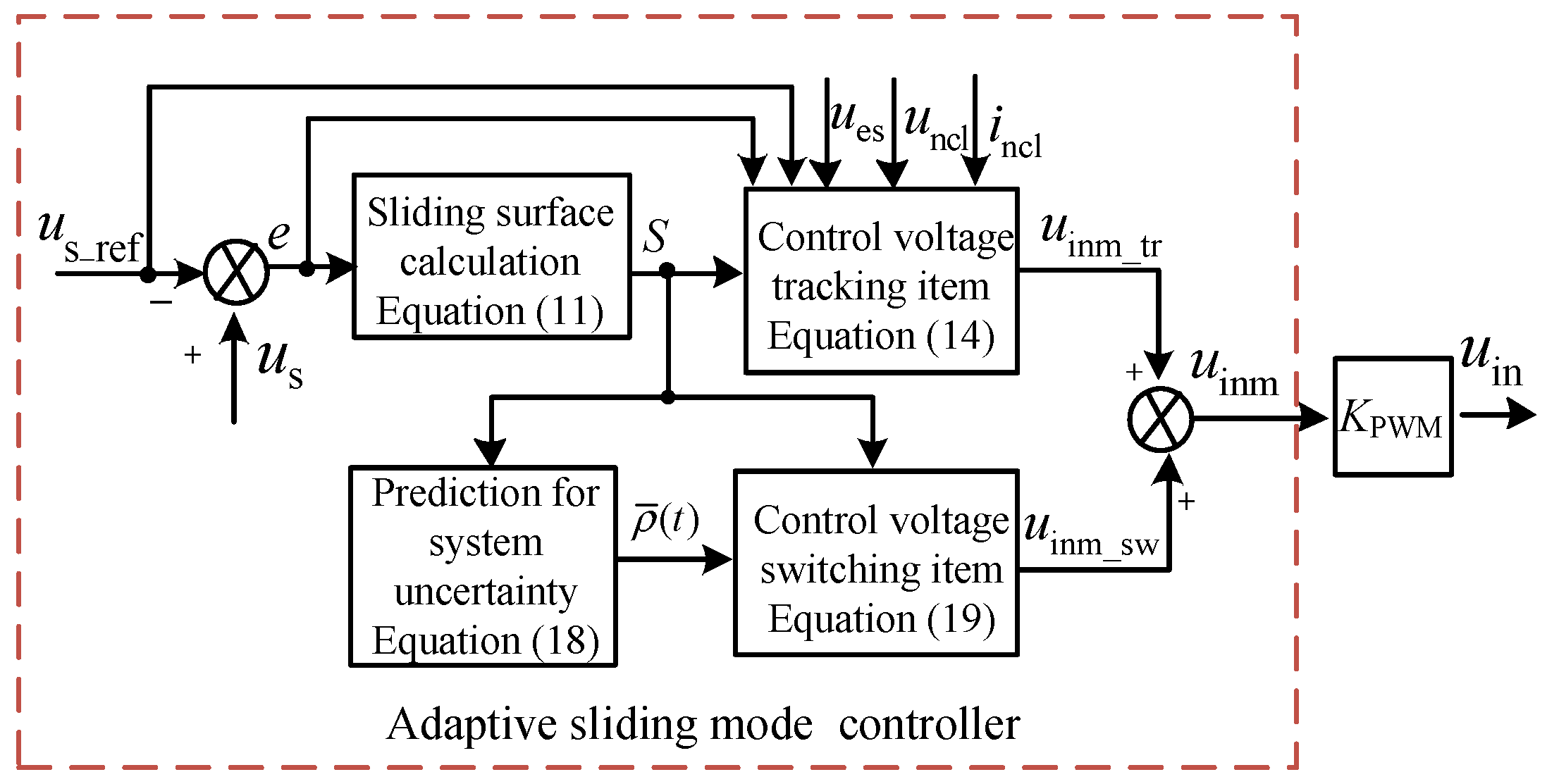
Figure 3 shows the ASMC strategy proposed herein. The red dotted frame shows the voltage controller, which is composed of the calculation module for the sliding surface, the prediction module for uncertainty, the control–voltage tracking item, and the control–voltage switching item. The voltage $u_{\mathrm{S}\_\mathrm{ref}}$ can be obtained from the calculation of the previous-level reference voltage, $e=u_{\mathrm{S}}-u_{\mathrm{S}\_\mathrm{ref}}$ is the voltage tracking error, and the pulse–width modulation wave $u_{\mathrm{inm}}$ is the sum of the control-voltage tracking item $u_{\mathrm{inm}\_\mathrm{tr}}$ and the control–voltage switching item $u_{\mathrm{inm}\_\mathrm{sw}}$. $S$ is the sliding surface function designed in this work, and $\overline{\rho }(t)$ is the variable part of the switching gain, which is related to the upper bound of the uncertainty of ES system. The sliding-surface calculation module computes in real-time $S$ according to the voltage error $e$. Provided the prediction module obtains the value of $S$, it can predict $\overline{\rho }(t)$. By using to $u_{\mathrm{es}}$, $u_{\mathrm{ncl}}$, $i_{\mathrm{ncl}}$, $e$, $u_{\mathrm{S}\_\mathrm{ref}}$, and $S$, the $u_{\mathrm{inm}\_\mathrm{tr}}$ can be computed by Equation (14) in real time. The $u_{\mathrm{inm}\_\mathrm{sw}}$ can be computed in real-time by Equation (19) according to $\overline{\rho }(t)$.

3.2. Design of the Adaptive Sliding-Mode Controller

The sliding-surface function is

$$S=\dot{e}+ce$$

(11)

where $c>0$ is a coefficient. Combining Equations (8) and (11) gives

$$\begin{array}{ll}\dot{S}& =\ddot{e}+c\dot{e}\\ & =\frac{1}{L{C}_{\mathrm{f}}}\left(K_{\mathrm{PWM}}{u}_{\mathrm{inm}}-u_{\mathrm{es}}\right)+\frac{{\dot{i}}_{\mathrm{ncl}}}{C_{\mathrm{f}}}+\omega (t)\\ & +{\ddot{u}}_{\mathrm{ncl}}-{\ddot{u}}_{{\mathrm{S}}_{-}\mathrm{ref}}+C(\left({\dot{u}}_{\mathrm{es}}+{\dot{u}}_{\mathrm{ncl}}-{\dot{u}}_{{\mathrm{S}}_{-}\mathrm{ref}}\right).\end{array}$$

(12)

Assume that the reaching law of sliding-mode control is

$$\dot{S}=-\tau S-\epsilon \mathrm{sgn}(S),$$

(13)

where $\tau$ and $\epsilon$ are positive constants. $\tau$ determines the rate at which the system state approaches the sliding surface (the smaller $\tau$ is, the lower the rate is). $\epsilon$ is the fixed part of the switching gain and correlates positively with the system-chattering amplitude.

Combining Equations (12) and (13), the controller can be designed as

$$\begin{array}{l}{u}_{\mathrm{inm}}=u_{\mathrm{inm}}{}_{\_\mathrm{sw}}+u_{\mathrm{inm}}{}_{\_\mathrm{tr}},\\ u_{\mathrm{inm}}{}_{\_\mathrm{sw}}=-K_{\mathrm{PWM}}^{-1}L{C}_{\mathrm{f}}(r+\epsilon )\mathrm{sgn}(S),\\ u_{\mathrm{inm}}{}_{\_\mathrm{tr}}=-K_{\mathrm{PWM}}^{-1}\left(L{C}_{\mathrm{f}}c\dot{e}-L{C}_{\mathrm{f}}{\ddot{u}}_{{\mathrm{S}}_{-}\mathrm{ref}}+L{C}_{\mathrm{f}}{\ddot{u}}_{\mathrm{ncl}}+L{\dot{i}}_{\mathrm{ncl}}-u_{\mathrm{es}}+L{C}_{\mathrm{f}}\tau S\right),\end{array}$$

(14)

where $r>0$ is a constant. Substituting Equation (14) into Equation (12) gives

$$S\dot{S}=S\left(\ddot{e}+c\dot{e}\right)=S\left[-(r+\epsilon )\mathrm{sgn}(S)-\tau S+\omega \left(\mathrm{t}\right)\right].$$

(15)

Take the Lyapunov function as

$$V_1=\frac{1}{2}{S}^2$$

(16)

and take the derivative of $V_1$ to obtain

$$\begin{array}{l}{\dot{V}}_1=S\dot{S}=-\tau {\mathrm{S}}^2-S(r+\epsilon )\mathrm{sgn}(S)+\omega (t)S\\ =-\tau S^2-(r+\epsilon )\left|S\right|+\omega (t)S\\ \le -\tau S^2-(r+\epsilon )\left|S\right|+\left|\omega (t)S\right|\\ =-\tau S^2-(r+\epsilon )\left|S\right|+\left|\omega (t)\right|\left|S\right|\\ =-\tau S^2-\epsilon \left|S\right|-\left[r-\left|\omega (t)\right|\right]\left|S\right|\\ \le -\left[r-\left|\omega (t)\right|\right]\left|S\right|.\end{array}$$

(17)

According to the Lyapunov stability theory, stabilizing the system requires ${\dot{V}}_1<0$. In other words, if the controller of Equation (14) is adopted, $r$ should be greater than the upper bound of the total uncertainty when considering the most severe disturbance of the ES system (i.e., $r>\rho$). However, in practice, the upper bound is difficult to determine in real-time, so only if $r$ is sufficiently large is it possible to ensure system stability. However, since the variable structure of sliding-mode control is mainly reflected in the chattering caused by the switching items, excessive switching gain ($r+\epsilon$) will lead to serious system chattering, which makes the motion of the system deviate significantly from the sliding surface and reduces the controller’s robustness.

In terms of system stability, the switching gain must be greater than the upper bound of the total uncertainty of the ES system to satisfy the condition for sliding-mode movement. In terms of control, the switching gain must be reduced to weaken chattering. The adaptive algorithm used herein can track disturbances in real-time and estimate the upper bound of the total uncertainty of the ES system. Taking this estimation as the variable part of the switching gain (replacing $r$) minimizes the switching gain, reduces chattering, and satisfies the condition for sliding-mode motion.

The adaptive law for estimating the upper bound of the total uncertainty is

$$\dot{\overline{\rho }}(t)=b\left|S\right|,$$

(18)

where $\overline{\rho }(t)$ is the estimated value of $\rho$, and $b>0$ is an adjustable coefficient. The rate of change of the estimated value can be changed by adjusting the value of $b$. Since $\dot{\overline{\rho }}(t)$ is related to the switching gain of the sliding-mode controller and directly affects the chattering of the system, an increasing $b$ is not better but should be considered comprehensively. Replacing $r$ in Equation (14) with $\overline{\rho }(t)$ allows the controller to be expressed as

$$\begin{array}{c}{u}_{\mathrm{inm}}=u_{\mathrm{inm}}{}_{\_\mathrm{sw}}+u_{\mathrm{inm}}{}_{\_\mathrm{tr}},\\ u_{\mathrm{inm}}{}_{\_\mathrm{sw}}=-K_{\mathrm{PWM}}^{-1}L{C}_{\mathrm{f}}\left[\overline{\rho }(t)+\epsilon \right]\mathrm{sgn}(S),\\ u_{\mathrm{inm}}{}_{\_\mathrm{tr}}=-K_{\mathrm{PWM}}^{-1}(L{C}_{\mathrm{f}}c\dot{e}-L{C}_{\mathrm{f}}{\ddot{u}}_{{\mathrm{S}}_{-}\mathrm{ref}}+L{C}_{\mathrm{f}}{\ddot{u}}_{\mathrm{ncl}}\\ +L{\dot{i}}_{\mathrm{ncl}}-u_{\mathrm{es}}+L{C}_{\mathrm{f}}\tau S).\end{array}$$

(19)

3.3. Stability Analysis

To prove the stability of the proposed control strategy, we use the following Lyapunov function:

$$V_2=\frac{1}{2}{S}^2+\frac{b^{-1}}{2}{\tilde{\rho }}^2,$$

(20)

where $\tilde{\rho }$ is the estimation error of the upper bound and is expressed as

$$\tilde{\rho }(t)=\overline{\rho }(t)-\rho .$$

(21)

Differentiating Equation (21) gives

$$\dot{\tilde{\rho }}(t)=\dot{\overline{\rho }}(t)=b\left|S\right|.$$

(22)

Differentiating the function $V_2$ gives

$$\begin{array}{ll}{\dot{V}}_2& =S\dot{S}+b^{-1}\tilde{\rho }\dot{\tilde{\rho }}\\ & =S\left[-(\overline{\rho }+\epsilon \left)\mathrm{sgn}\right(S)+\omega (t)-\tau S\right]+b^{-1}\tilde{\rho }\dot{\tilde{\rho }}\\ & =-S(\overline{\rho }+\epsilon \left)\mathrm{sgn}\right(S)+\omega (t)S-\tau S^2+b^{-1}\tilde{\rho }\dot{\tilde{\rho }}\\ & =-\left|S\right|(\overline{\rho }+\epsilon )+\omega (t)S-\tau S^2+b^{-1}\tilde{\rho }\dot{\tilde{\rho }}\\ & =-\left|S\right|\overline{\rho }-\left|S\right|\epsilon +\omega (t)S-\tau S^2+b^{-1}\tilde{\rho }\dot{\tilde{\rho }}\\ & \le -\left|S\right|\overline{\rho }-\left|S\right|\epsilon +\left|\omega (t)\right|\left|S\right|-\tau S^2+b^{-1}\tilde{\rho }\dot{\tilde{\rho }}\\ & \le -\left|S\right|\overline{\rho }-\left|S\right|\epsilon +\rho \left|S\right|-\tau S^2+b^{-1}\tilde{\rho }\dot{\tilde{\rho }}\\ & =(\rho -\overline{\rho })\left|S\right|-\epsilon \left|S\right|+b^{-1}\tilde{\rho }\dot{\tilde{\rho }}.\end{array}$$

(23)

Substituting Equations (21) and (22) into Equation (23) gives

$$\begin{array}{cc}\hfill {\dot{V}}_2& \le \tilde{\rho }\left(b^{-1}\dot{\tilde{\rho }}-\left|S\right|\right)-\epsilon \left|S\right|\hfill \\ & =-\epsilon \left|S\right|\le 0.\hfill \end{array}$$

(24)

Equations (20) and (24) show that $V_2$ is positive definite and ${\dot{V}}_2$ is negative semi-definite. When $\left|S\right|\ne 0$, $V_2>0$ and ${\dot{V}}_2<0$, the ES system is thus asymptotically stable.

When the system state reaches the sliding mode area and remains on the sliding surface, we have $S=\dot{S}=0$, and the equivalent control of ES can be computed by applying Equation (12):

$$u_{\mathrm{inm}}{{}_{-}}_{\mathrm{eq}}=\frac{L{C}_{\mathrm{f}}}{K_{\mathrm{PWM}}}\left[{\ddot{u}}_{{\mathrm{S}}_{-}\mathrm{ref}}+\frac{u_{\mathrm{es}}}{L{C}_{\mathrm{f}}}-\frac{{\dot{i}}_{\mathrm{ncl}}}{C_{\mathrm{f}}}-{\ddot{u}}_{\mathrm{ncl}}-C\dot{e}-\omega (t)\right].$$

(25)

Substituting Equation (25) into Equation (8) gives

$$\ddot{e}=-c\dot{e}.$$

(26)

Equation (26) shows that, provided the coefficient $c$ is properly designed, the system is in a sliding-mode state and the CL voltage can be adjusted. In summary, the adaptive sliding-mode controller designed herein ensures the asymptotic stability of the ES system.

4. Simulations

To verify the effectiveness and anti-interference ability of the proposed ASMC strategy, we use a simulation model (see Figure 2) parametrized as shown in

Table 1. Simulation parameters for the electrical and control systems of the ES.

Parameter	Value
RMS of us_ref/V	220
R1/Ω	0.179
L1/mH	1.2
Zcl/Ω	50
Zncl/Ω	3
L /mH	3
Cf /uF	50
UDC/V	350
fs/kHz	20
$\tau$/103	120
$\epsilon$	350
b	2
C/103	100

.

When the RMS of $u_{\mathrm{S}\_\mathrm{ref}}$ is set to 220 V, the given model parameters produce $U_{\mathrm{g}\_\mathrm{ref}}=235.7\hspace{0.17em}\mathrm{V}$. Therefore, the supply-side voltage is chosen as 214.5 V ($0.91U_{\mathrm{g}\_\mathrm{ref}}$) and 240.4 V ($1.02U_{\mathrm{g}\_\mathrm{ref}}$) to simulate the situation for lower or higher $U_{\mathrm{g}\_\mathrm{ref}}$.

4.1. Verification of Performance of Voltage Stabilization

The first simulation verifies the voltage stabilizing performance of the ASMC strategy and compares the results with the linear controller (PR and PI). In this part, the switch S_W is disconnected before 0.3 s, and the ES is only connected in series into the system in the form of capacitor $C_f$. At 0.3 s, S_W is connected and $u_{\mathrm{S}}$ is controlled.

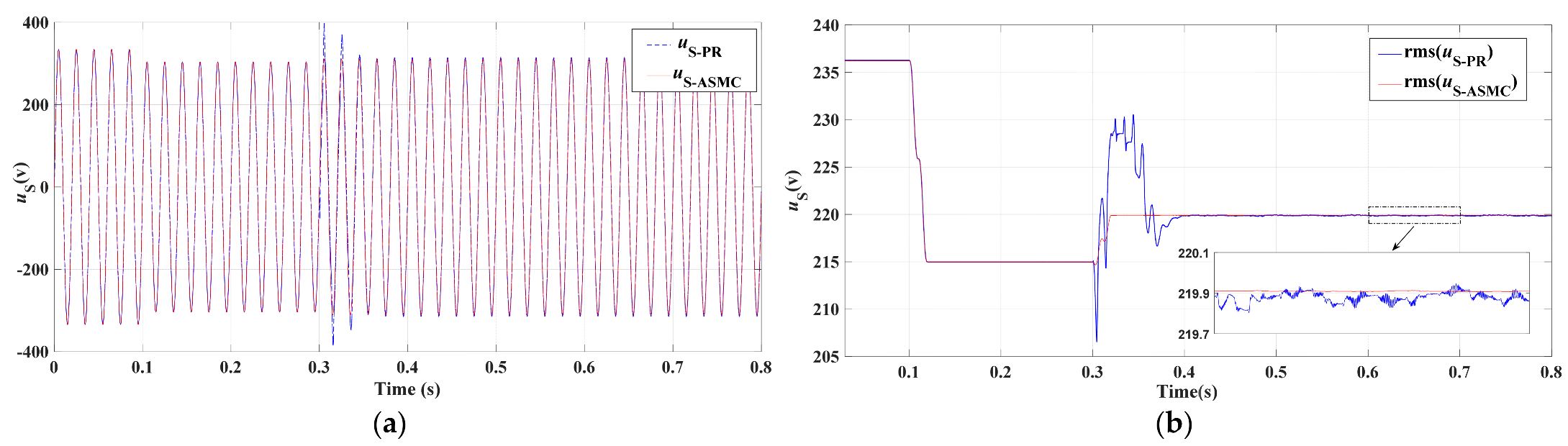
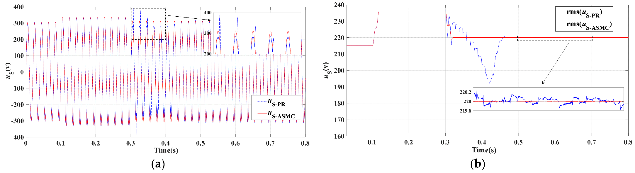
Figure 4 shows the voltage stabilization due to the two control strategies when the ES operates in capacitive mode. Since the ES does not control $u_{\mathrm{S}}$ before 0.3 s, $u_{\mathrm{S}}$ follows $u_{\mathrm{g}}$ and is not stabilized at 220 V. The RMS of $u_{\mathrm{g}}$ is 214.5 V after 0.1 s, lower than $U_{\mathrm{g}\_\mathrm{ref}}$, so the ES works in capacitive mode after being connected. Figure 4 shows that both control strategies effectively control $u_{\mathrm{S}}$ after the ES is connected. The instantaneous value waveform remains sinusoidal, and the RMS is stable at about 220 V. Comparatively, the ASMC strategy (the red line) makes $u_{\mathrm{S}}$ more rapidly reach the steady state; the transition time is only about 0.02 s, and the RMS overshoot for $u_{\mathrm{S}}$ is almost zero. However, the transient period of the system under PR control (see blue line) is longer by about 0.1 s, and the overshoot is significantly larger. These results indicate that the ASMC strategy produces better dynamic performance. Expanding the steady-state part of Figure 4b shows that, under the ASMC strategy, the RMS of $u_{\mathrm{S}}$ is a straight line very close to 220 V, and the steady-state error is smaller. Under PR control, the RMS waveform oscillates in the range of 0.3 V, which shows that the ASMC strategy produces a better static performance than PR control.

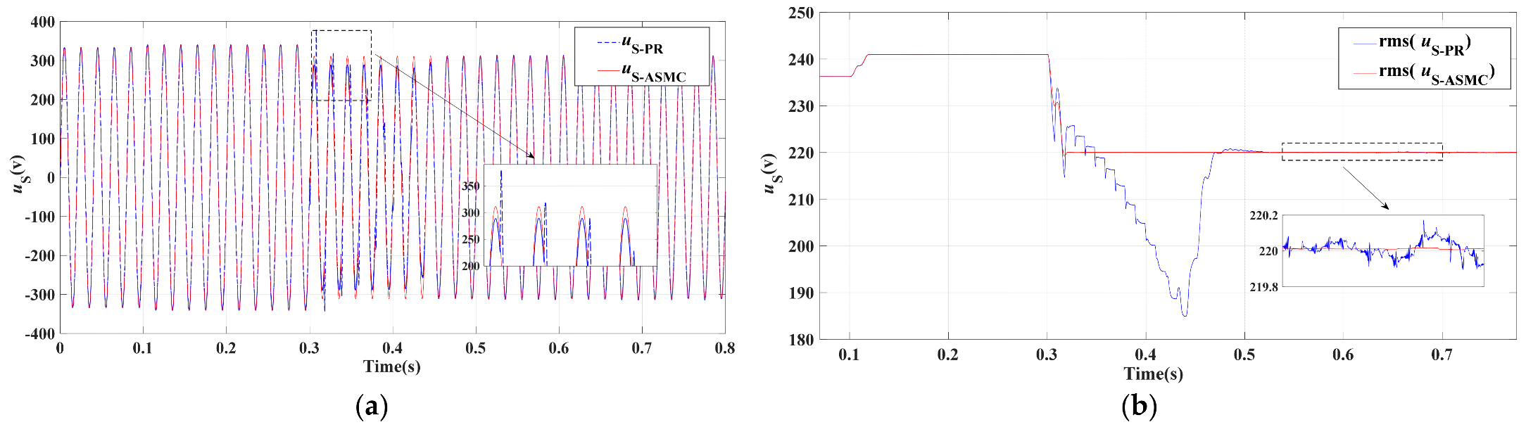
Figure 5 shows the voltage stabilization due to the two control strategies when the ES operates in resistive mode. During the time interval 0–0.3 s, $u_{\mathrm{S}}$ changes with $u_{\mathrm{g}}$. When the ES is connected at 0.3 s, the RMS of $u_{\mathrm{g}}$ is 235.7 V, so the ES works in resistive mode. During the time interval 0.1–0.3 s, although the RMS of $u_{\mathrm{g}}$ equals $U_{\mathrm{g}\_\mathrm{ref}}$, the ES is not connected and is only embedded in the system as a capacitor, so u_S is not 220 but 236.2 V. Figure 5 shows that, in resistive mode, the ES under PR control and the proposed ASMC strategy still stabilizes the CL voltage, and the instantaneous waveform remains sinusoidal. At the same time, compared with PR control, the ASMC strategy also greatly shortens the transition period (PR control takes 0.18 s, whereas ASMC control takes 0.02 s), and the overshoot is also significantly reduced. This situation is like the ES working in capacitive mode.

Expanding the relevant part of Figure 5 shows that, under the proposed ASMC strategy, the instantaneous waveform remains sinusoidal during the transition period, and the RMS of $u_{\mathrm{S}}$ stabilizes at 220 V after the system is stabilized. However, under PR control, the instantaneous waveform is significantly distorted during the transition period, and the RMS of $u_{\mathrm{S}}$ oscillates within the range of 220 ± 0.2 V in the steady state. This analysis shows that, when the ES works in resistive mode, the ASMC strategy can effectively stabilize the CL voltage and the dynamic and static performances are better than PR control.

Figure 6 shows that the RMS of $u_{\mathrm{S}}$ is 236.2 V in the time interval 0–0.1 s. After 0.1 s, the RMS of $u_{\mathrm{g}}$ is set to 240.4 V, so the RMS of $u_{\mathrm{S}}$ rises to 241 V, and the ES works in inductive mode after being connected at 0.3 s. As shown in Figure 6, both control strategies stabilize the CL voltage when the ES works in inductive mode, just like the capacitive and resistive modes. Comparatively, the ASMC strategy in this mode still produces better dynamic and static performance. For example, the transition period of u_S takes 0.25 s under PR control. During this period, not only is the voltage waveform severely distorted, but the RMS drops to 185 V. However, under the ASMC strategy, the voltage waveform is always sinusoidal, the transition period only takes 0.02 s, and the minimum RMS is 219.2 V. Expanding the steady-state part in Figure 6 shows that, under the ASMC strategy, the RMS of $u_{\mathrm{S}}$ is stable at 220 V. However, under PR control, the situation is like the case when the ES works in capacitive mode, and the RMS oscillates in a range of ±0.2 V around 220 V.

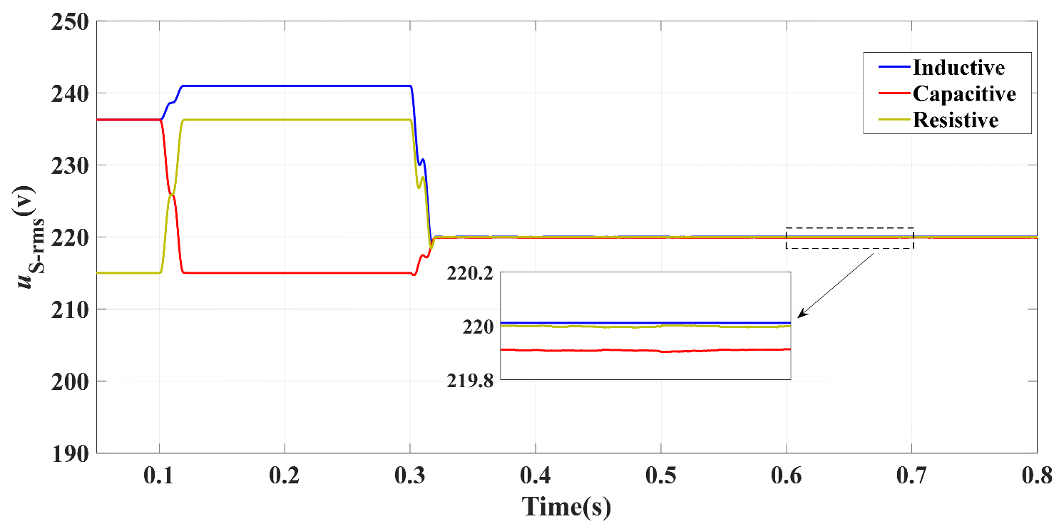
Figure 7 shows the voltage stabilization of ES when using a saturation function for $u_{\mathrm{inm}\_\mathrm{sw}}$. As shown in Figure 7, when operating in any of the three modes, ES quickly stabilizes the RMS of $u_{\mathrm{S}}$ at about 220 V. The smooth curves and tiny chattering reflect the superior performance. The steady-state error in capacitive mode is slightly larger than in the other two modes.

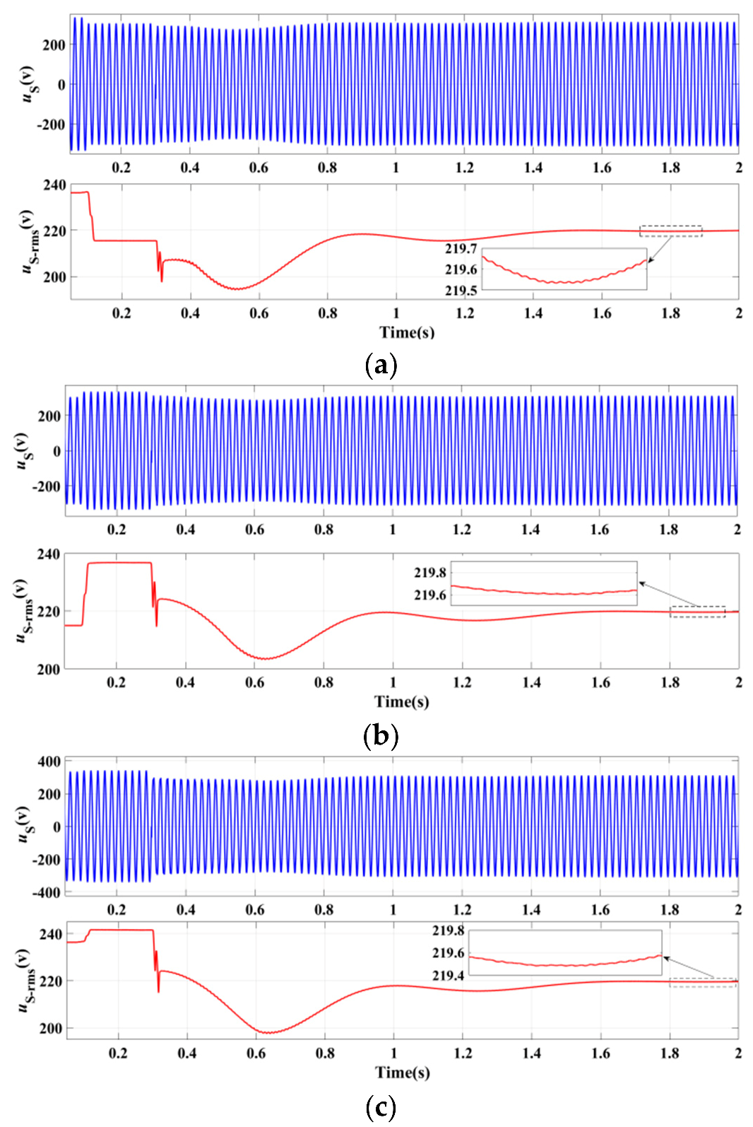
Figure 8a–c show the $u_{\mathrm{S}}$ waveform and its RMS curve when the ES uses the PI controller to work in the capacitive mode, resistive mode, and inductive mode, respectively. Consistent with PR control and ASMC, S_W is also closed at 0.3 s. Figure 8 shows that the ES uses the PI controller to keep the waveform of $u_{\mathrm{S}}$ sinusoidal and the RMS stable at 220 V in the different modes. However, the adjustment time in all three modes exceeds 1.5 s, and the maximum deviation of the RMS is 17 V. These two pieces of data are much greater than the corresponding values for the ASMC.

The analysis of Figure 4, Figure 5, Figure 6, Figure 7 and Figure 8 shows that the proposed ASMC strategy stabilizes the CL voltage and produces a faster response speed and smaller steady-state error than PR or PI control.

4.2. Verification of Anti-Interference Performance

This section verifies the anti-interference ability of the ASMC strategy and then compares the results with PR and PI control. In this part, the ES is always connected. When the ES adopts PR control or ASMC, during the time interval 0–0.1 s, the supply-side voltage is set to $U_{\mathrm{g}\_\mathrm{ref}}$, which is 235.7 V. After 0.1 s, the RMS of $u_{\mathrm{g}}$ drops to 214.5 V, and the disturbance is added to the system at 0.3 s. Since the PI control has a longer adjustment time, when the ES adopts the PI control, the above two action times are set at 2 and 4.5 s, respectively, with the other parameters remain unchanged.

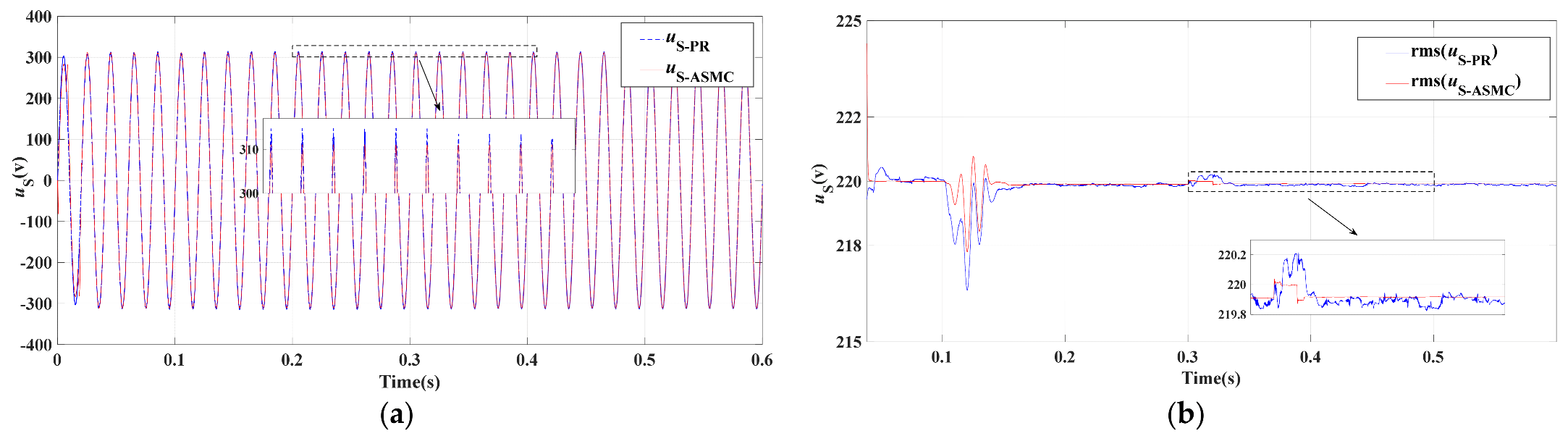
Figure 9 shows that both the ASMC and PR control can keep the RMS of CL voltage at about 220 V before 0.3 s, but the waveform amplitude of the latter more clearly exceeds 311 V. At 0.3 s, the inductor $L$ changes from 3 to 6 mH. Under the ASMC strategy, $u_{\mathrm{S}}$ is hardly affected, its waveform is a smooth sine wave, and its RMS can be stabilized quickly. Comparatively, the ability of PR control to resist parameter perturbation is weaker. The RMS waveform has been oscillating, and the time to reach the steady state is slightly longer. The overshoot of the RMS is larger, and the steady-state error is also larger.

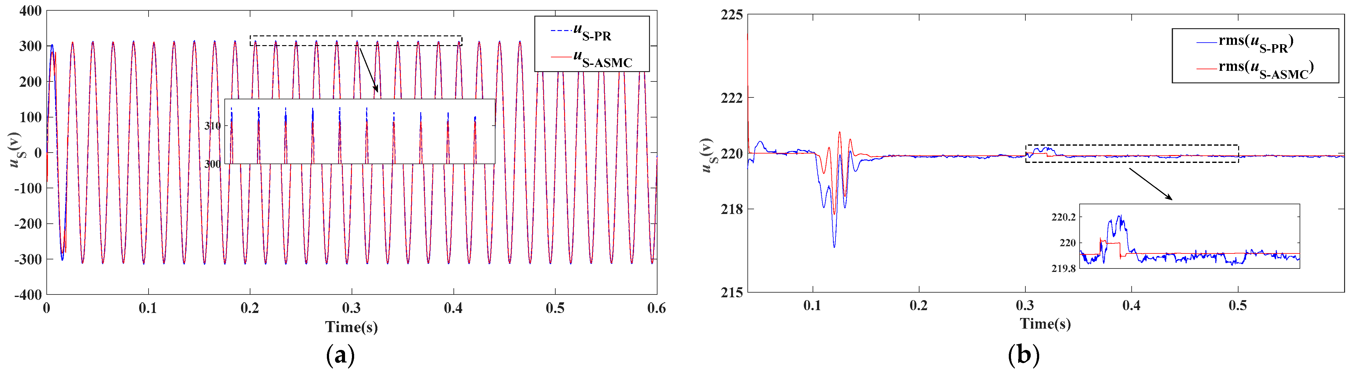
In Figure 10, the DC side voltage suddenly drops from 350 to 320 V at 0.3 s. Like Figure 9, before 0.3 s, the CL voltage is maintained at about 220 V under the two control strategies. After $U_{\mathrm{DC}}$ changes suddenly, both control strategies maintain the $u_{\mathrm{S}}$ waveform sinusoidal. Expanding this figure further shows that, under the ASMC strategy, $u_{\mathrm{S}}$ is almost unaffected by variations in $U_{\mathrm{DC}}$; it stabilizes within 20 ms, and the RMS of $u_{\mathrm{S}}$ is only 0.03 V lower than before $U_{\mathrm{DC}}$ drops. However, under PR control, the transition period is slightly longer, and the RMS of u_S oscillates between 219.7 and 220 V.

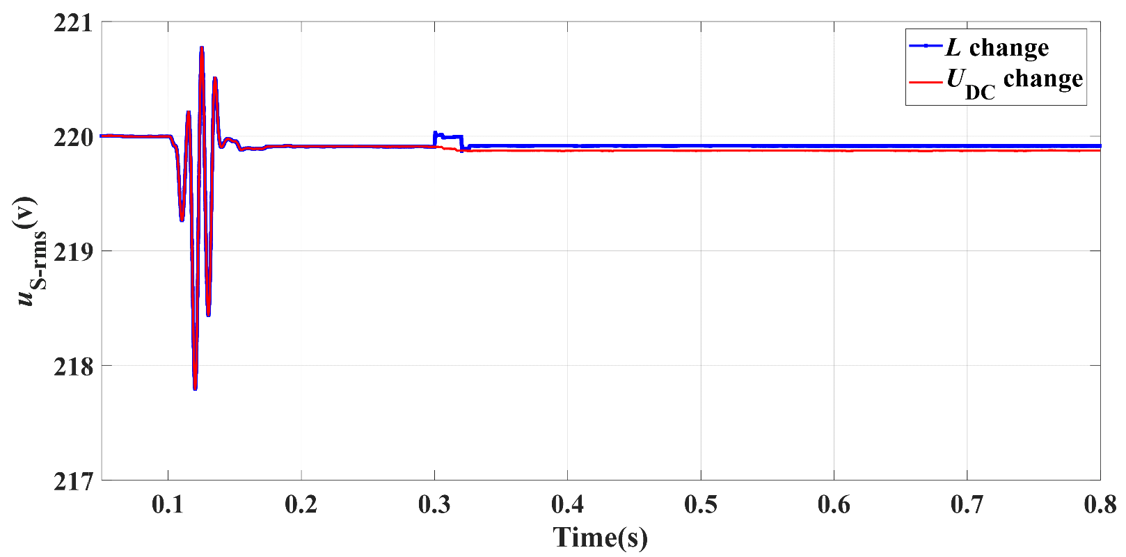
Figure 11 shows the anti-interference ability of the ASMC strategy when the control–voltage switching item uses a saturation function. As shown in this figure, L or $U_{\mathrm{DC}}$ suddenly changes at 0.3 s, and the CL voltage stabilizes at about 220 V within a very short time. When ES reaches the steady state, almost no chattering occurs. This result indicates that the ASMC strategy also performs well when $u_{\mathrm{inm}\_\mathrm{sw}}$ uses a saturation function.

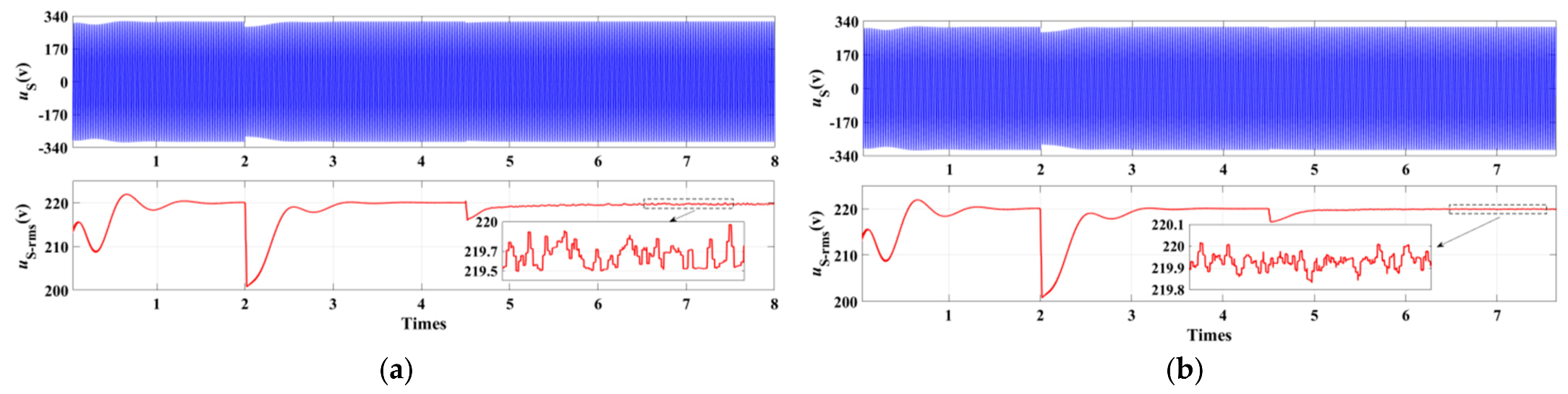
Figure 12 shows the anti-interference ability of the ES using the PI controller. Like ASMC or PR control, PI control stabilizes $u_{\mathrm{S}}$ at 220 V before interference is added to the system. Figure 12a shows that it takes about 2 s to stabilize $u_{\mathrm{S}}$ after $L$ changes, whereas this time interval is only 2 ms under the ASMC strategy. Enlarging the relevant part of Figure 12a reveals that a steady-state error oscillates in the range of 0.5 V. Figure 12b shows that the RMS of $u_{\mathrm{S}}$ drops to 217.2 V when $U_{\mathrm{DC}}$ suddenly decreases, and stabilizes at about 220 V after 1 s. Like when $L$ changes, the steady-state error oscillates in the range of 0.2 V.

The analyses of Figure 9, Figure 10, Figure 11 and Figure 12 show that the proposed ASMC strategy is more resistant to parameter perturbation and external disturbance, and its robustness is better than linear control.

5. Conclusions

In an ES control system, the conventional linear controller has poor robustness against uncertain disturbances of the system. To solve this problem, we design herein an adaptive sliding-mode control system based on predicting the total uncertainty disturbance of the ES system. The results of Matlab simulations lead to the following conclusions:

(1)

The ES operates in three modes when using the proposed ASMC strategy to stabilize the critical load voltage at the target value. When the system has uncertain disturbances, such as parameter perturbations or external disturbances, this strategy is more robust and ensures that the critical load voltage retains a good waveform and that the RMS is stable.

(2)

Comparing the simulation results of the PR and PI controls and of the ASMC shows that, with or without considering the system uncertainty disturbances, the latter strategy shortens the adjustment time, reduces the overshoot and the steady-state error, and produces better dynamic and static performance.