Deep Learning Neural Networks for Short-Term PV Power Forecasting via Sky Image Method

Abstract

Solar photovoltaic (PV) power generation is prone to drastic changes due to cloud cover. The power is easily affected within a very short period of time. Thus, the accuracy of grasping cloud distribution is important for PV power forecasting. This study proposes a novel sky image method to obtain the cloud coverage rate used for short-term PV power forecasting. The authors developed an image analysis algorithm from the sky images obtained by an on-site whole sky imager (WSI). To verify the effectiveness of cloud coverage rate as the parameter for PV power forecast, four different combinations of weather features were used to compare the accuracy of short-term PV power forecasting. In addition to the artificial neural network (ANN) model, long short-term memory (LSTM) and the gated recurrent unit (GRU) were also introduced to compare their applicability conditions. After a comprehensive analysis, the coverage rate is the key weather feature, which can improve the accuracy by about 2% compared to the case without coverage feature. It also indicates that the LSTM and GRU models revealed better forecast results under different weather conditions, meaning that the cloud coverage rate proposed in this study has a significant benefit for short-term PV power forecasting.

1. Introduction

Solar photovoltaics (PVs) have an intermittent characteristic and are easily affected by the climate environment, cloud cover, and sunlight intensity. These weather conditions will cause the instability of renewable energy power generation [1]. Therefore, it is imperative to provide good weather forecasting to master the power generation of renewable energy. Furthermore, the weather parameters in different forecasting time horizons are also slightly different. The input meteorological factors of short-term forecasting are usually cloud cover and wind direction. The weather parameters of medium-term forecasting are temperature, humidity, irradiance intensity, wind speed, and wind direction from the site of some meteorological equipment in the local area. For the long-term forecasting, the long-term observation data of the weather forecast needs to be considered [2,3]. There have been many studies that have explored the influence of weather parameters on the accuracy of PV power forecasting. This research includes finding the best weather influencing factor, comparing the forecasting deviation under different weather, or adding parameters that worsen the forecasting results [4,5,6,7].

The cloud coverage and solar irradiation prediction are the important weather parameters that directly influence the variety of solar photovoltaic power from minutes to hours. The cloud coverage and solar irradiation can be obtained from the analysis of the sky image. In solar irradiance prediction, image pixels are processed to identify clear/thin/thick clouds, the function of the solar pixel angle (SPA), image zenith angle (IZA), and solar zenith angle (SZA) [8,9,10]. In addition, the solar irradiation prediction value is obtained through analyzing the difference in the picture pixel brightness, the difference in the continuous picture pixel and cloud image trajectory, and used as one of the learning parameters for solar photovoltaic forecasting [11,12,13,14,15].

However, pyrheliometer equipment is installed in most of the PV plants, which can easily obtain the ultra-violet index (UVI) value, which represents the solar radiation index. Therefore, the prior research directly used the sky image to analyze the cloud trajectory or cloud cover and directly used it as a forecasting method for PV power generation. In particular, Zhang et al. [16] used CNN, integrating sky images by stacking four exposures in grayscale images for the 60 s before the current time t with a 15 s interval. The result showed that using the LSTM-based model yielded a 21% RMSE skill score that outperformed other approaches. Kong et al. [17] proposed a novel approach based on deep whole-sky-image learning architectures for 4 to 20 min of solar photovoltaic generation forecasting. The experimental results showed that the hybrid static image forecaster provided superior performance, up to an 8.3% improvement in general and up to 32.8% improvement in the cases of ramp events when compared to that without sky images. Both Wang et al. and Zhen et al. [18,19] proposed a hybrid mapping model for solar PV power forecasting, and their models yielded higher accuracy than the CNN, LSTM, and ANN models. In the data processing, they filtered the noises of the original sky image and reduced the image resolution. However, they trained the dataset in three different ways including color images with a 3D form, stitching of the three R, G, B channels, and all pixel values of the image. On the other hand, Wen et al. [20] used the sky image parameter in solar photovoltaic prediction for industrial applications. The results showed that it could be used as a reference basis for smooth photovoltaic power generation control upon cloudy and sunny days, thereby reducing the energy curtailment. Furthermore, the sky image analysis methods they used are complicated and difficult to implement. Therefore, the present sky image analysis method is much simpler and easier to implement in this paper.

This paper proposes a new and interesting image pixel calculation formula for image processing. It obtains the cloud coverage rate per minute based on the defined threshold as one of the PV power forecasting parameters. The advantage of the proposed method in comparison with the previous literature is that these values are easy to parse and sequence for the time series model. Furthermore, the collected data can be easily integrated with other weather data quickly and introduced into the PV forecasting deep learning model to learn and forecast. In particular, the cloud coverage rate can improve the PV power forecasting accuracy of this study. The structure of this article is as follows. Section 2 describes the solar photovoltaic forecasting framework and the local weather equipment. Section 3 focuses on the proposed sky image coverage analysis method, and the deep learning models are introduced. Section 4 presents and discusses the experimental results with different weather combinations. Finally, Section 5 concludes this article.

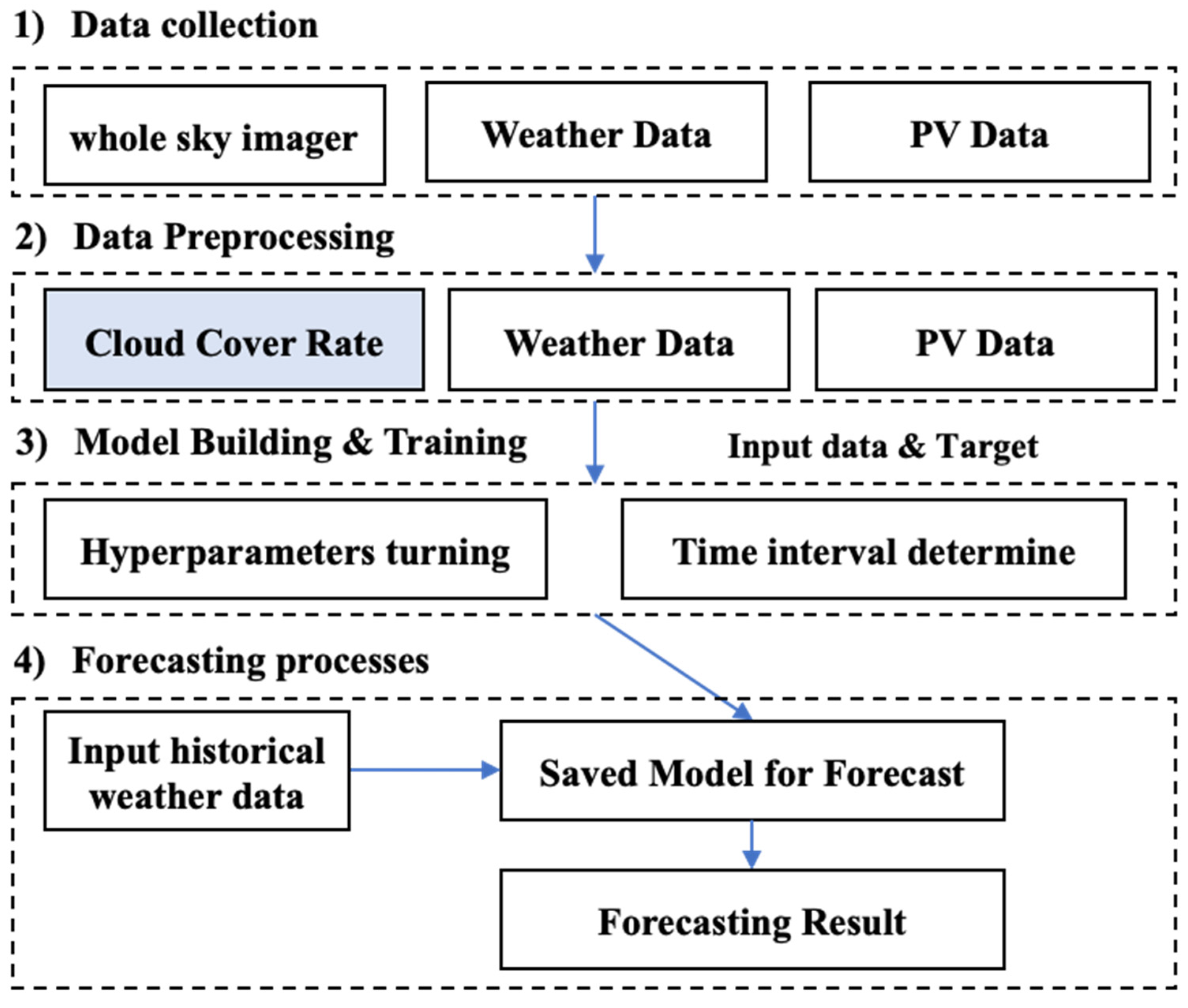
2. Forecasting Procedures and Data Set

In this section, the PV forecasting operation procedures is introduced, as shown in Figure 1, which contains four main processes including the data collection, data processing, model building and training, and forecasting processes. The details are described as follows.

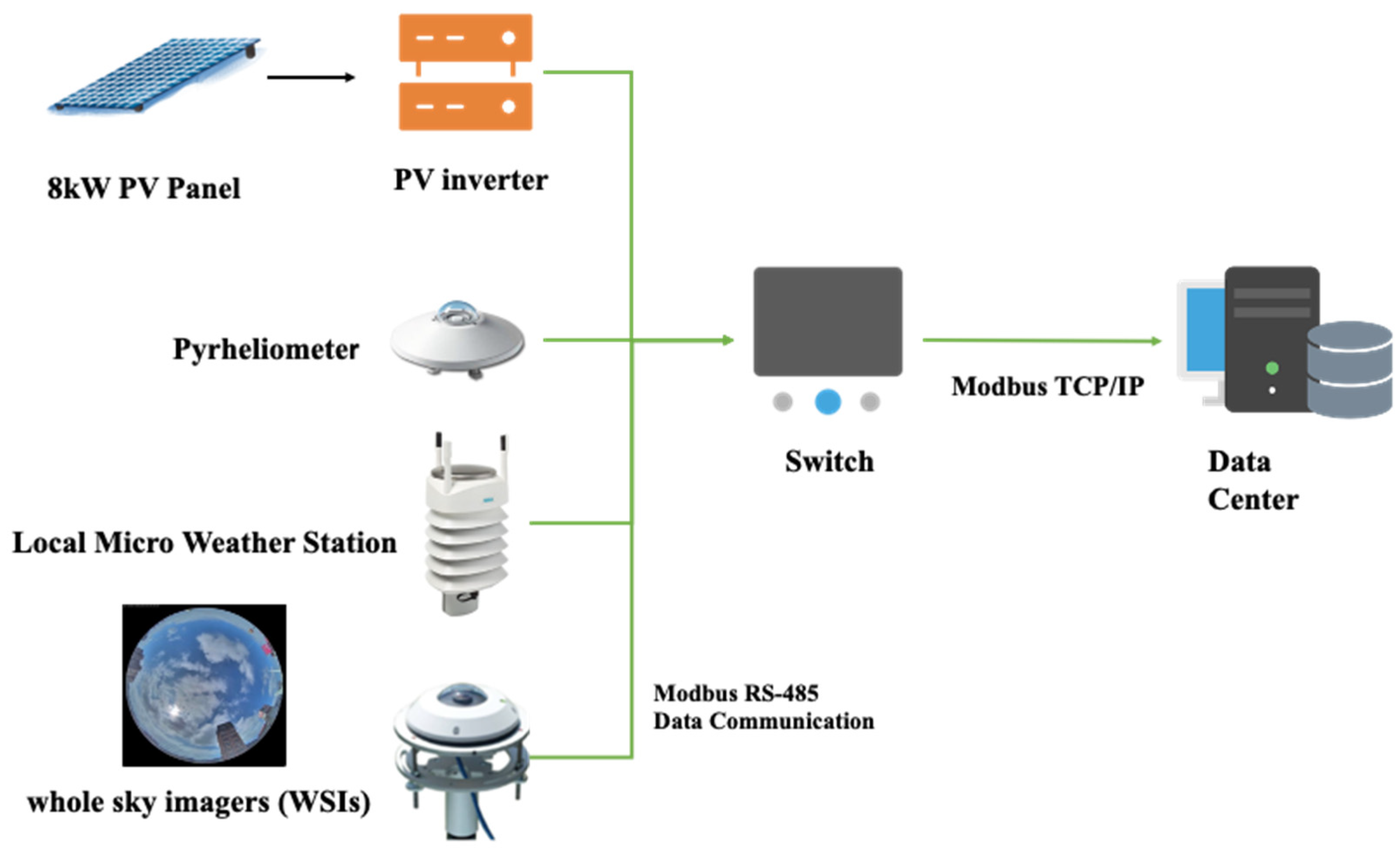
2.1. Data Collection

The equipment used for data collection in this paper is shown in Figure 2 including the power data of the 8 kW PV plants, the UVI data from the pyrheliometer, local micro weather station (contains wind speed and direction, temperature, relative humidity), and the whole sky imager (WSI). Furthermore, in the overall dataset in this study, the collection period of the weather and PV data was from 21 February 2021 to 13 June 2021.

2.2. Data Processing

The purpose of the present work was to calculate the cloud coverage rate through the sky image. For simplicity, the authors preprocessed the sky image to exclude the unnecessary objects in the image including trees, buildings, and the outside black areas of the image. Then, the information was fed into the proposed RGB sky image processing method. This pretreatment converts each image into a numerical data type. It calculates the cloud coverage rate as the weather characteristic value. In the meantime, the proposed method also preprocesses the weather data from the local small weather station and examines whether it contains missing data to ensure the photovoltaic data integrity.

2.3. Model Building and Training Processes

Establishing a deep learning model: The deep learning neural network model based on the ANN, LSTM, and GRU model were applied in this study. In addition, determining the model hyperparameters is essential. Thus, the parameter turning of hidden units, training steps, and epochs are incorporated to ensure that there is no overfitting of these models to maintain the suitability and predictive accuracy of hyperparameters.

2.4. Forecasting Processes

This part uses the model that has already trained hyperparameter and weights for short-term PV power forecasting. On the other hand, the authors used four different weather feature combinations and verified the prediction performance of cloud coverage rate as the parameter for short-term PV power forecasting including Case 1: Six weather values (wind speed and direction, UVI, temperature, relative humidity, coverage rate); Case 2: Five weather value (without coverage rate); Case 3: Five weather values (without UVI); and Case 4: Only coverage rate and relative humidity. The predictive abilities of these three models for short-term PV power forecasting were compared in the final result.

3. Methodology

A new sky image analysis method for short-term PV power generation forecasting is proposed in this article. In this section, sky image coverage processing, the cloud computing method, deep learning models (ANN, LSTM, GRU), and evaluation indices will be introduced separately.

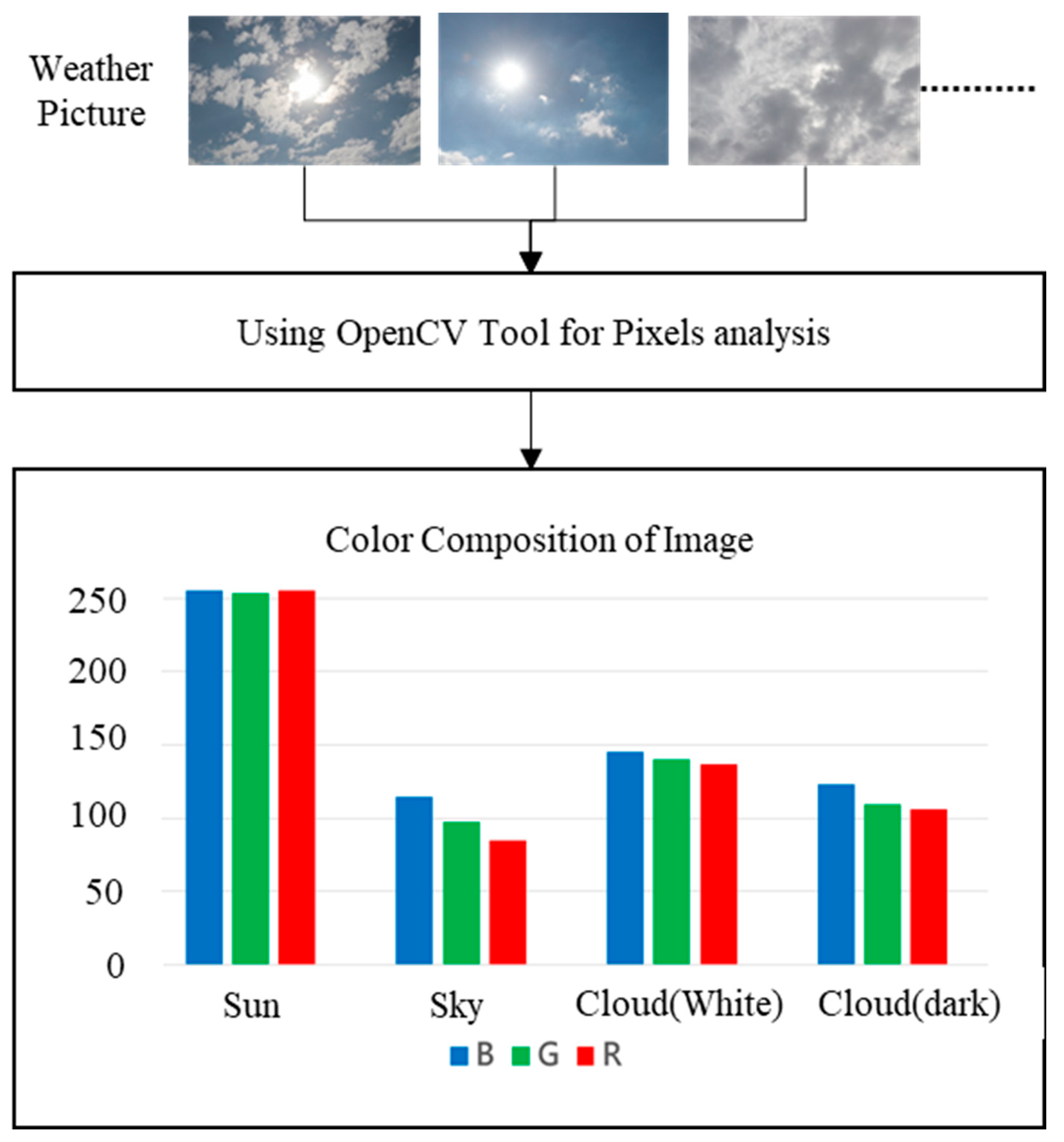
3.1. Sky Image Coverage Processing Method

The sky image processing of this research focuses on RGB pixel composition. In RGB, the grayscale color refers to converting a color picture into a grayscale picture that is still not far from the original color, as shown in Equation (1). Since each picture is composed of different color components, the authors defined Δ (pixel composition) to represent the three combined color difference results, and is expressed in Equation (2):

$$\mathrm{R}\approx \mathrm{G}\approx \mathrm{B}$$

(1)

$$\Delta ={\left(\mathrm{R}-\mathrm{G}\right)}^2+{\left(\mathrm{R}-\mathrm{B}\right)}^2+{\left(\mathrm{G}-\mathrm{B}\right)}^2$$

(2)

Furthermore, to perform the RGB distribution analysis of each element image under different weather patterns and to analyze the sunny, mostly clear, and cloudy images before performing the sky image analysis, the authors adopted the Open-Source Computer Vision (OpenCV) library in python to analyze the sky image and determine the RGB distribution ratio. The analysis and statistical results are shown in Figure 3.

After analyzing the color composition, the difference between the blue and green pixels is about one δ variable. Moreover, the difference between blue and red pixels is about two δ variables, and the mathematical relationship between the three combined colors is listed in Equation (3). Substituting Equation (3) into Equation (2), subject to some mathematical manipulation, yields Equation (4).

$$\forall \mathsf{\delta }\in \mathbb{N}:\left(\mathrm{B}-\mathrm{G}\right)=\mathsf{\delta }\Rightarrow \left(\mathrm{B}-\mathrm{R}\right)\cong 2\mathsf{\delta }$$

(3)

$$\Delta ={\left(\mathsf{\delta }\right)}^2+{\left(4\mathsf{\delta }\right)}^2+{\left(\mathsf{\delta }\right)}^2$$

(4)

The statistical analysis shows that the change in Δ is mainly because of the color difference between the red and blue pixels. Therefore, the deviation in the green pixel in the sky image analysis occurs. In order to maintain the same importance among the three pixels (R, G, B), the authors employed the weighting coefficient method to adjust the relationship of the three pixels. Finally, this study proposes the general mathematical formula of the RGB analysis method as follows:

$$\Delta =4\times {\left(\mathrm{R}-\mathrm{G}\right)}^2+{\left(\mathrm{R}-\mathrm{B}\right)}^2+4\times {\left(\mathrm{G}-\mathrm{B}\right)}^2$$

(5)

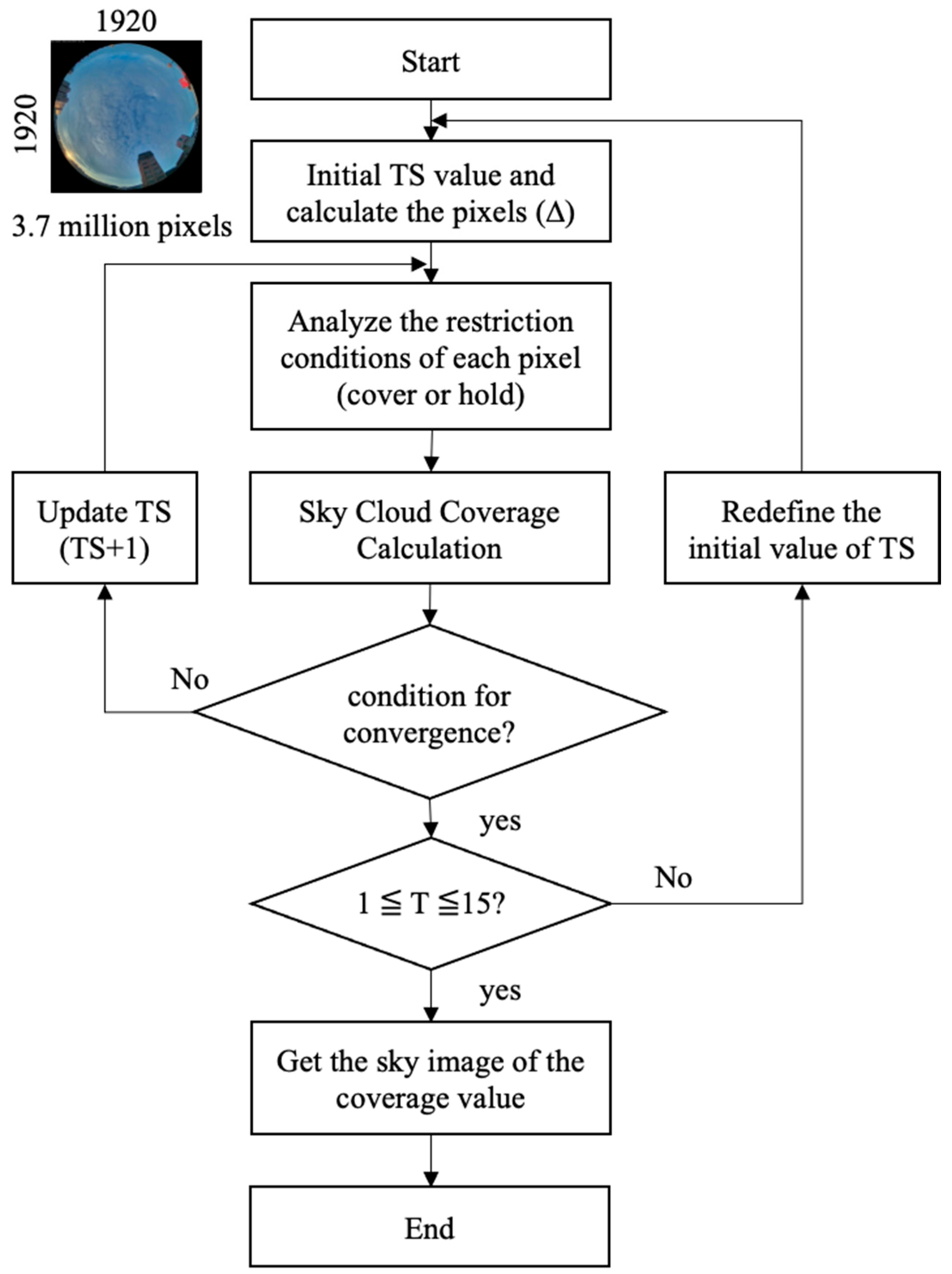
3.2. Cloud Covering Analysis Structure and Calculation Method

The cloud covering analysis structure is shown in Figure 4. This process can be divided into the following four parts:

(1)

Calculate the Pixel Composition

Calculate the pixel composition and set up the initial threshold (TS) value: The pixel composition is determined by Equation (5). The initial value of TS is random, and it will increase by one after each cycle until the coverage condition is reached.

(2)

Define the Sky Image Covering Limiting

Define the sky image covering limiting condition: By analyzing the pixel composition, the authors defined the limit condition of the sun, clouds, and sky as listed in

Table 1. The sky image covering limiting condition.

Item	Limit Condition	Pixel Status	Pixel Status
Δ (pixel composition) ≥ Threshold (TS)	$\sum \left(R,G,B\right)>760$	Sun	Remain
	$\sum \left(R,G,B\right)\le 760$	Cloud	Cover
Δ (pixel composition) < Threshold (TS)	B > R ∩ B > G	Sky	Remain
	Others	Ex: Tree	Cover

. Sunny conditions prevail when the pixel composition exceeds TS, and the R, G, B elements are greater than 760. Conversely, it is regarded as cloudy if the value is less than 760. Furthermore, sky conditions occur if the pixel composition is less than or equal to TS and the blue value is larger than the red and green values at the same time.

(3)

Cloud Covering Calculation

The authors defined the cloud coverage rate in Equation (6). In addition, there will be a similar coverage rate in a specific range by analyzing the time-series sky images through testing. Therefore, when the coverage rate increases and the slope decreases, the program will record the coverage rate as the current value in this cycle.

Table 2. The results of the automatic convergence.

TS	Sky Image Cover Result	Coverage Rate
12		32.52%
14		44.83%
16		45.95%
18		61.53%

depicts the result of the automatic convergence example. From this table, when TS is 16, the cloud coverage rate is 49.95%, and when TS is 18, the cloud coverage rate changes by 15%. In addition, the sky image shows that it will be over-covered when the coverage rate = 61.53% and the TS = 18, thereby revealing the non-cloud situations.

$$\mathrm{Cloud} \mathrm{coverage} \mathrm{rate}(\%)=[1-\frac{\left(\mathrm{all} \mathrm{pixels}-{\mathrm{mask}}^{\prime }\mathrm{s} \mathrm{pixels}-{\mathrm{cloud}}^{\prime }\mathrm{s} \mathrm{pixels}\right)}{\left(\mathrm{all} \mathrm{pixels}-{\mathrm{cloud}}^{\prime }\mathrm{s} \mathrm{pixels}\right)}]$$

(6)

(4)

Update the Threshold Value

Update the threshold value: In this study, updating the threshold value for every 15 min was adopted to accelerate the cloud image analysis. Through the testing experience, each coverage analysis was about 6 to 7 s, which was sufficient for short-term photovoltaics forecasting.

3.3. Choice of The Deep Learning Model

The authors used artificial neural networks and recurrent neural network models to train and predict the PV power, which are the ANN, LSTM, and GRU models. The ANN model has a strong nonlinear fitting ability and strong adaptive ability. The LSTM can control the transmission state through the gated state, remembering the unimportant information that needs to be remembered for a long time. The GRU has the same effect as LSTM, but needs fewer parameters to build models with a large amount of training [21,22,23].

The models have their advantages in training and forecasting. During the training process, all choices were performed by trying different hyperparameters on the same training set including hidden units, training steps (Epochs), and input time intervals. Thus, the authors will discuss which model is more suitable for this field based on the short-term PV power forecast results in this paper.

3.4. Evaluation Indices

The forecasting performance of PV power prediction models is evaluated using three statistical indicators, which are the mean absolute error (MAE), root mean squared error (RMSE), and mean absolute percentage error (MAPE) [24]. Their corresponding formulas are given by Equations (7)–(9):

$$\mathrm{MAE} =\frac{1}{N}\sum _{i=1}^N|\widehat{X_i}-X_i|$$

(7)

$$\mathrm{RMSE} =\sqrt{\frac{1}{N}\sum _{i=1}^N{(\widehat{X_i}-X_i)}^2}$$

(8)

$$\mathrm{MAPE} =\frac{1}{N}\sum _{i=1}^N|\frac{X_i-\widehat{X_i}}{X_i}|\times 100\%$$

(9)

where $\widehat{X_i}$ and $X_i$ represent the ith forecasted and actual value, respectively, and N is the size of the test dataset.

4. Numerical Results

This section evaluates the influence of the coverage rate under different weather conditions on the performance of one-hour ahead PV power generation forecasting. The numerical results were comprehensively compared and subsequently discussed.

4.1. Results of Sky Image Processing by RGB Formula

This study proposed two RGB formulas (Equations (2) and (5)) for the sky image processing. In this section, the authors simulated and compared the threshold ratio of Equations (2) and (5), which is (1 + 1 + 1):(4 + 1 + 4) = 1:3. Therefore, in the sky image analysis, the threshold values will represent TS = n × 30 and TS = n × 90, where n is a constant 1, 2, 3…. Note that it is quite challenging to analyze the difference between the two RGB analysis methods on sunny days because there were fewer clouds under sufficient sunlight. However, there was a noticeable difference in cloudy days. Specifically, when n increased continuously, the difference in cloud covering will become more apparent, as shown in

Table 3. The results of the RGB comparison on a sunny day.

Index	Equations (2): TS = n × 30	Equations (5): TS = n × 90
n = 1
n = 2
n = 3

and

Table 4. The results of the RGB comparison on a cloudy day.

Index	Equations (2): TS = n × 30	Equations (5): TS = n × 90
n = 1
n = 2
n = 3

. The result indicates that Equation (5) is superior to Equation (2), especially on a cloudy day. From the result, Equation (5) is more sensitive and accurate, and it is the main RGB formula used in this article.

4.2. Results of Adjust Hyperparameters

The adjustment of hyperparameters in deep learning has a specific impact on the training and predictive results. Therefore, the authors first used 21 days of weather information (starting from 24 February) for training and testing including hidden units, training steps (Epochs), and input time intervals to find the most suitable hyperparameter combinations for the three models (ANN, LSTM, GRU). All data were sorted by the minute. The fixed parameters were learning rate (learning rate: 1 × 10⁻³) and batch size (batch size: 16). Finally, three evaluation indices (MAE, RMSE, and MAPE) were used to evaluate the model. The results showed that the ANN model used five hidden layers, the number of Epochs was 3000, and data input interval was one hour; in the LSTM model, it used seven hidden layers, the number of Epochs was 2500, and the data input interval was 2 h; in the GRU model, it used six hidden layers, the number of Epochs was 1500, and data input interval was 3 h. The results of the hyperparameter adjustment are shown in

Table 5. The results of the adjustment of the hyperparameters.

Index	Model	Adjust Parameters			Fixed Parameters		Evaluation
		Input Time	Layers	Epochs	Learning Rate	Batch Size	MAE	RMSE	MAPE
1	ANN	1 h	5	3000	$1\times {10}^{-3}$	16	0.026	0.046	18.94%
2	LSTM	2 h	7	1500	$1\times {10}^{-3}$	16	0.027	0.049	14.33%
3	GRU	3 h	6	2500	$1\times {10}^{-3}$	16	0.015	0.030	10.54%

.

4.3. Performance Comparison with Different Weather Features on Sunny and Cloudy Days

The four different weather feature combinations for short-term solar photovoltaic forecast analysis are as follows. Case 1: Six weather features (wind speed and direction, UVI, temperature, relative humidity, coverage rate); Case 2: Five weather features (without coverage rate); Case 3: Five weather features (without UVI), and Case 4: Only coverage rate and relatively humidity. These cases aim to study whether the cloud coverage proposed in this paper can reduce the use of features and promote the accuracy of the PV power generation forecasts.

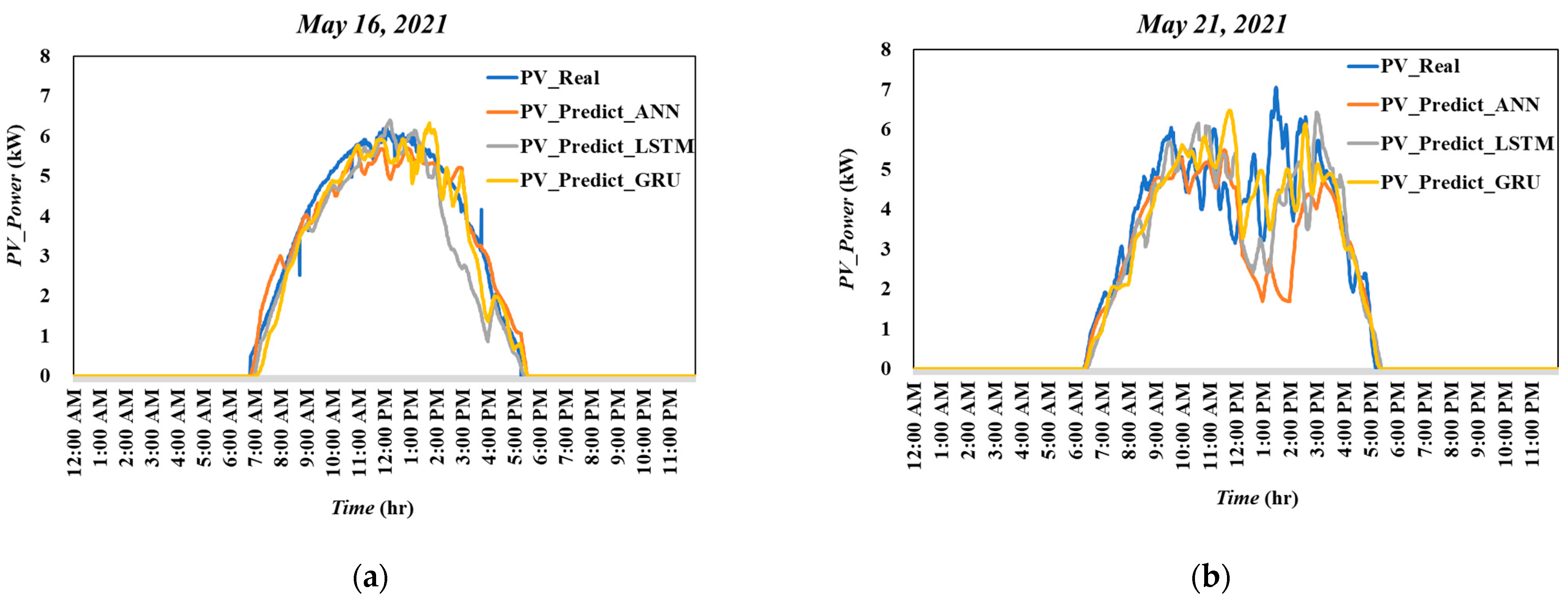
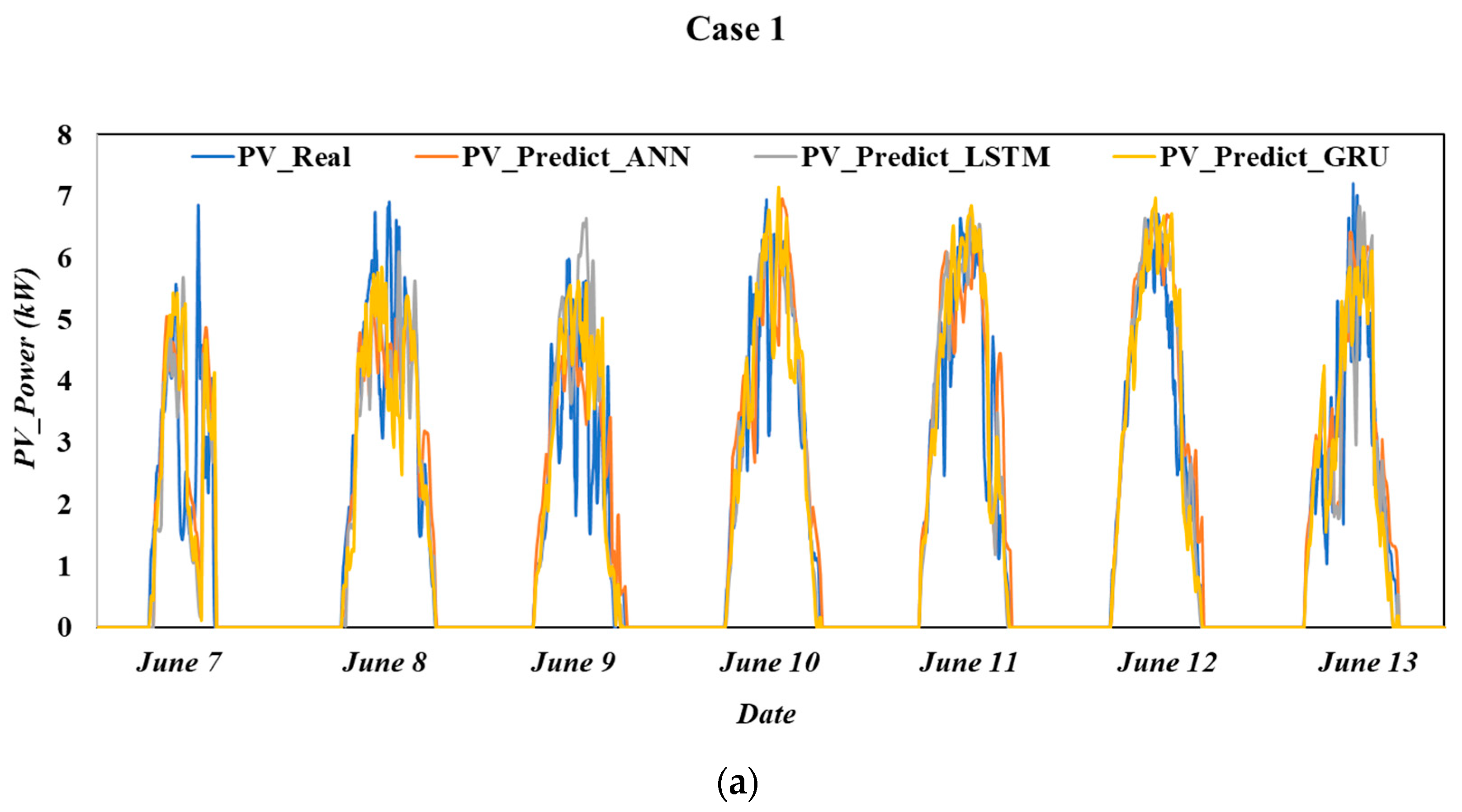
4.3.1. Case 1: Results of Six Weather Features

In this case, there were six weather features of the dataset: wind speed and direction, UVI, temperature, relative humidity, and coverage rate. Figure 5 intuitively shows the PV forecast results of the three models on sunny and mostly cloudy days. The best forecasting model was ANN on sunny days, which is more consistent with the actual tracked solar photovoltaic power generation. In addition, the GRU and LSTM yielded large predictive deviations between 3 and 4 PM, respectively. The preliminary assessment may be the interaction between the weather parameters. On the other hand, it can be found that the predictive result of ANN varied widely on mostly cloudy days. In contrast, the prediction trend of LSTM and GRU was better. There are two possible reasons for this difference. First, the time series forecasting model was more adaptable in the large ramp up and ramp down situation. Second, there were less data of cloudy days and poor weather. As a result, the ANN model showed insufficient experience upon prediction.

Further evaluation and analysis results are shown in

Table 6. Case 1. The results of the six weather features.

Index	Model	Six Weather Values
		Sunny			Cloudy			Average
		MAPE%	MAE	RMSE	MAPE%	MAE	RMSE	MAPE%	MAE	RMSE
1	ANN	6.544	0.017	0.029	11.763	0.052	0.115	9.154	0.035	0.072
2	LSTM	8.869	0.024	0.046	12.439	0.046	0.088	10.654	0.035	0.067
3	GRU	7.779	0.019	0.032	10.253	0.039	0.078	9.016	0.029	0.055

. The result indicates that there was a better prediction effect of ANN under sunny conditions, with a MAPE of 6.54%, MAE of 0.017, and RMSE of 0.029. In contrast, the prediction effect of GRU was better under cloudy conditions with a MAPE of 10.25%, MAE of 0.039, and RMSE of 0.078. Based on the average of the two-day forecast results, it was found that GRU performed better, with a MAPE of 9.02%, MAE of 0.029, and RMSE of 0.055.

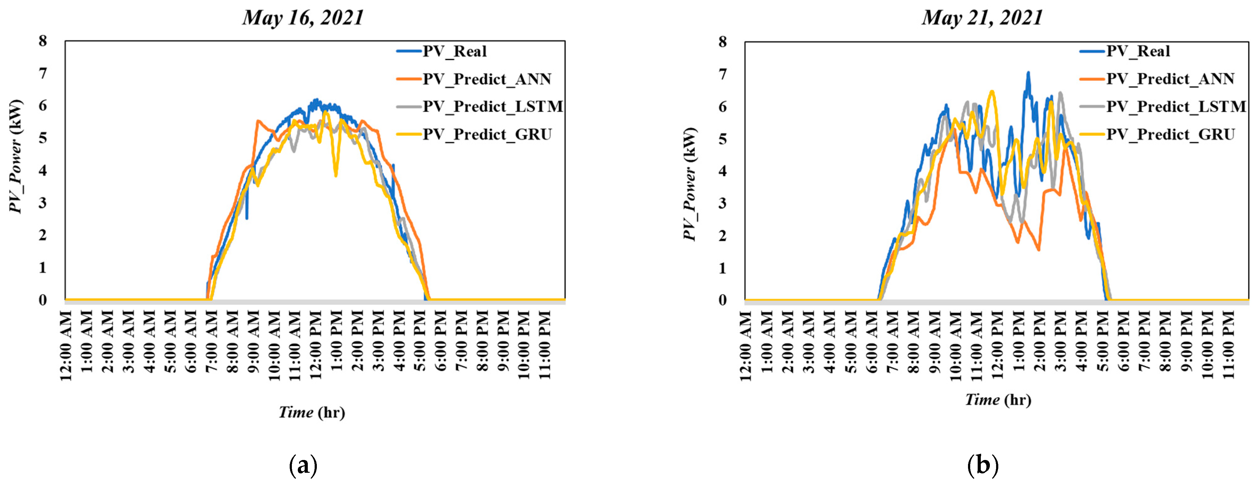
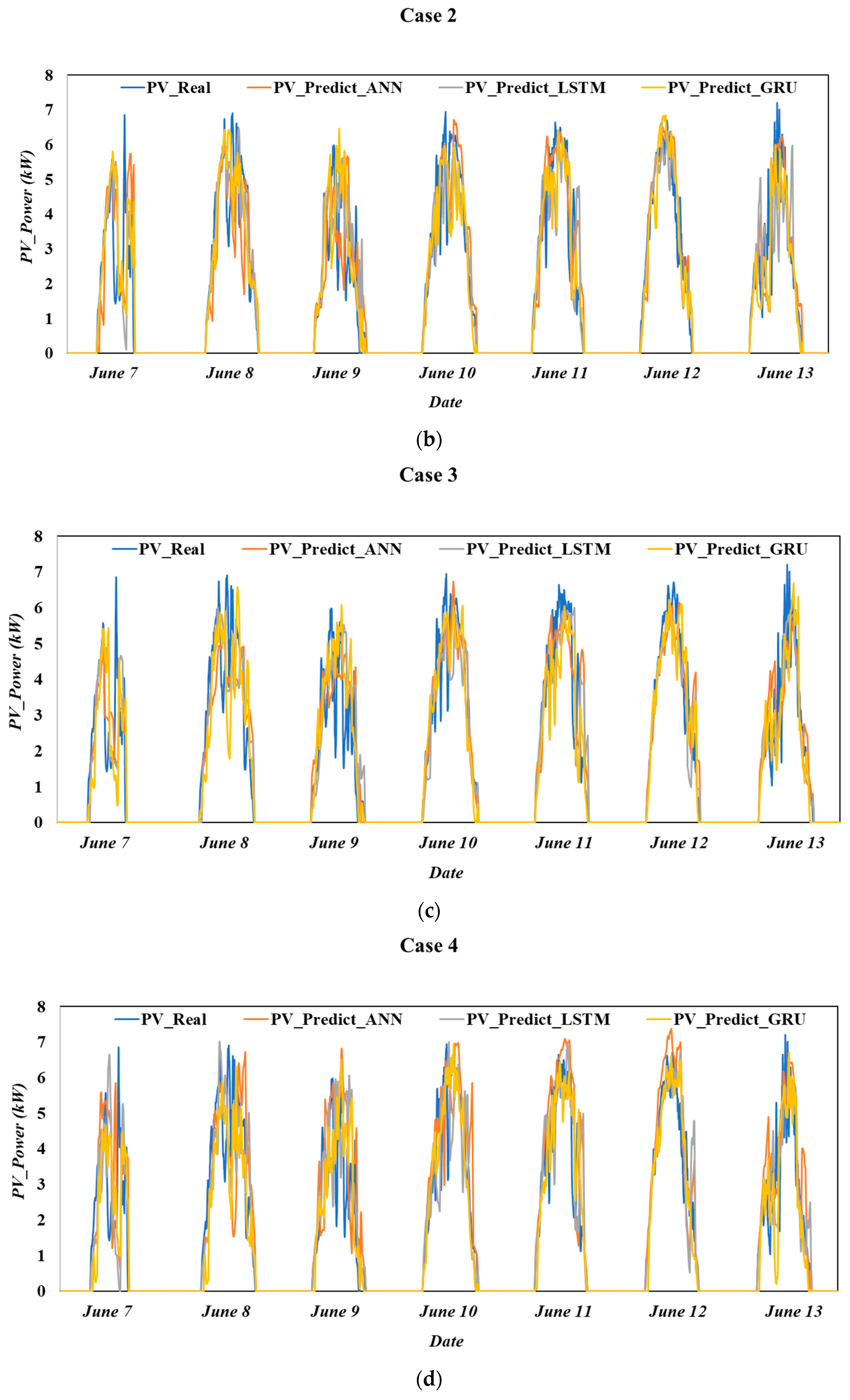
4.3.2. Case 2: The Results of Five Weather Features (without Coverage Rate)

In this case, there were five weather features of the dataset: wind speed and direction, UVI, temperature, relative humidity. The predictive results are shown in Figure 6. In the sunny condition, it can be found that the solar photovoltaic power curve predicted by ANN significantly deviated from the actual one due to a lack of the cloud coverage rate. The deviation occurred in the interval of 9 to 10 AM and 2 to 3 PM. Furthermore, the GRU model also revealed a significant forecast departure at 1 PM. However, the prediction trend of LSTM was close to the actual PV power curve. Under mostly cloudy conditions, the forecast trends of the ANN and GRU models deviated significantly from the actual curve, especially between 1:30 to 2:30 PM. In contrast, the predictive results of the LSTM model were only slightly different from Case 1.

Table 7. Case 2. The results of five weather values (without coverage rate).

Index	Model	Five Weather Value (without Coverage Rate)
		Sunny			Cloudy			Average
		MAPE%	MAE	RMSE	MAPE%	MAE	RMSE	MAPE%	MAE	RMSE
1	ANN	7.857	0.019	0.032	16.251	0.071	0.135	12.054	0.045	0.084
2	LSTM	7.233	0.020	0.035	12.861	0.049	0.101	10.047	0.035	0.068
3	GRU	7.628	0.022	0.039	15.953	0.0614	0.122	11.791	0.042	0.081

describes the forecasting results of the three models on sunny and mostly cloudy days. In the sunny day, the ANN still outperformed other models where MAPE was about 7.85%, MAE was 0.019, and RMSE was 0.032. Under the mostly cloudy condition, the accuracy of the LSTM model was about 2 to 3% higher than the others.

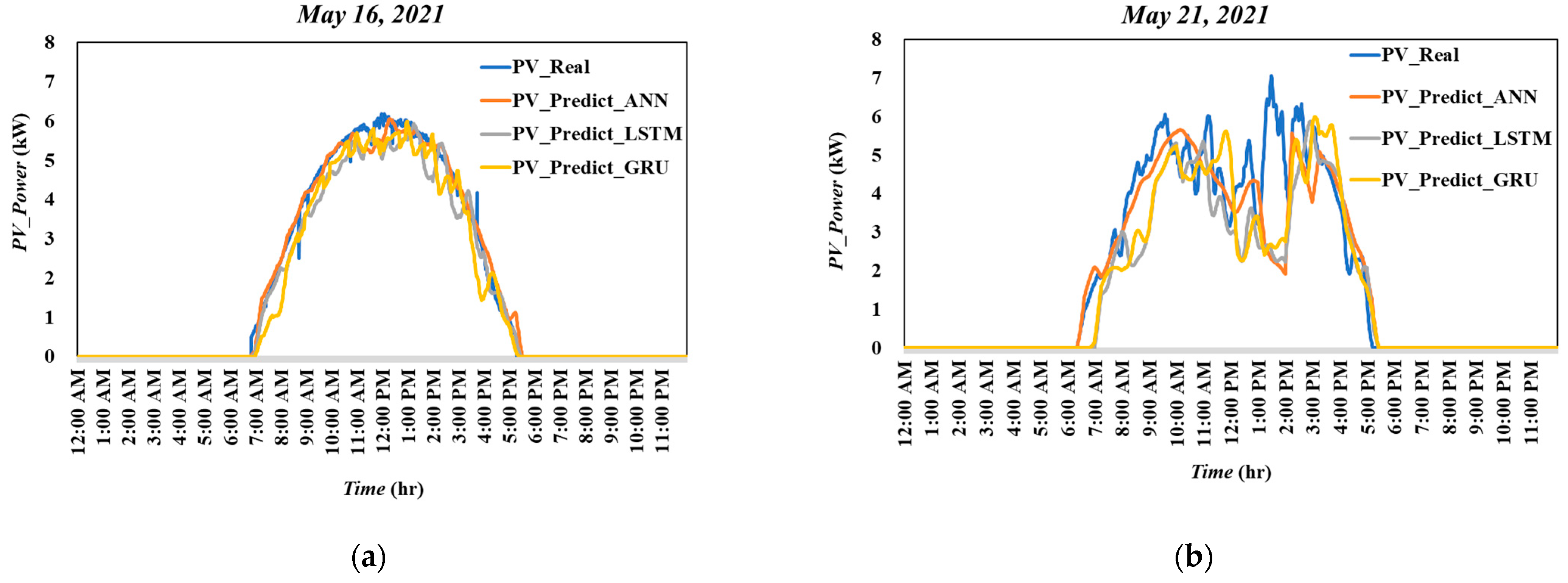
4.3.3. Case 3: Results of Five Weather Feature (without UVI)

Five weather features except for UVI were used in this case. The results of the prediction are shown in Figure 7. Compared with the actual curve, the prediction trend of the three models was roughly the same when the UVI was removed under sunny conditions, which was quite different from those of removing the coverage rate. Therefore, the coverage rate was the dominant feature that influences the predictive performance in the sunny condition. On the other hand, under a mostly cloudy condition, the performance of the three models was not significantly different from that in Case 2.

The further evaluation and analysis results are summarized in

Table 8. Case 3. The results of five weather values (without UVI).

Index	Model	Five Weather Values (without UVI)
		Sunny			Cloudy			Average
		MAPE%	MAE	RMSE	MAPE%	MAE	RMSE	MAPE%%	MAE	RMSE
1	ANN	4.001	0.009	0.019	11.492	0.041	0.096	7.747	0.025	0.058
2	LSTM	6.023	0.019	0.033	15.749	0.057	0.114	10.886	0.038	0.074
3	GRU	8.799	0.021	0.036	15.902	0.587	0.112	12.351	0.304	0.074

. The forecast evaluation indices were significantly improved when the coverage rate was included, and this is applicable even without the UVI feature. Based on the average forecasting results of the different weather conditions, the overall forecasting effect of ANN was better than the other models, with a MAPE of 7.7%, a MAE of 0.025, and an RMSE of 0.058, respectively.

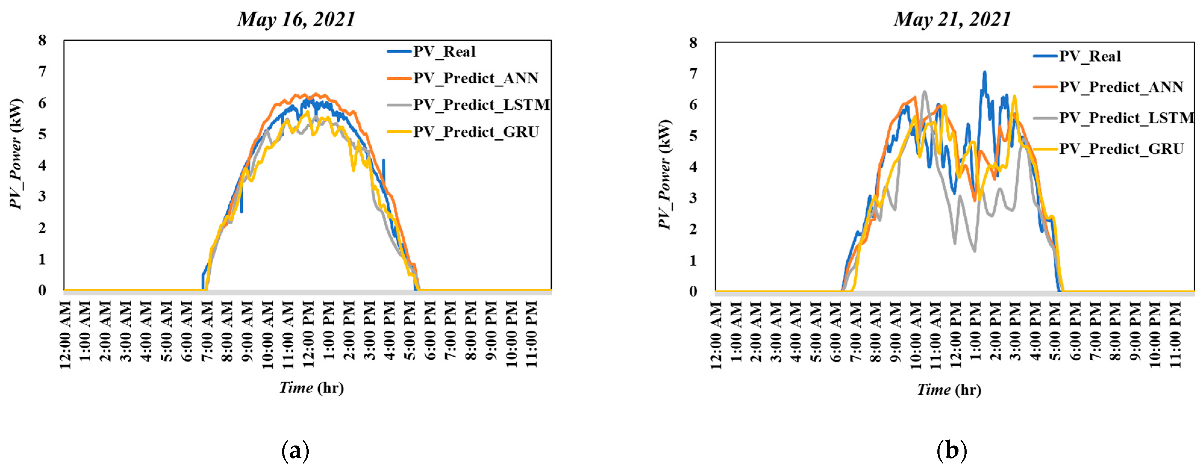
4.3.4. Case 4: The Results of Only Coverage Rate and Relative Humidity

In this case, only the relative humidity and coverage rate features of the dataset were used in the prediction. Figure 8 shows the forecast result of the three models subjected to sunny and mostly cloudy weather. In the sunny condition, either ANN, LSTM, or GRU all showed good predictive ability, in particular, the prediction curve of ANN almost coincided with the trajectory of the real PV power curve. The prediction curves of ANN and GRU were close to the actual curve between 1:30 PM to 2:10 PM.

Table 9. Case 4. The results of the only coverage rate and relatively humidity.

Index	Model	Only Coverage Rate and Relatively Humidity
		Sunny			Cloudy			Average
		MAPE%	MAE	RMSE	MAPE%	MAE	RMSE	MAPE%	MAE	RMSE
1	ANN	3.933	0.008	0.015	10.342	0.036	0.069	7.138	0.022	0.042
2	LSTM	7.195	0.021	0.035	15.377	0.069	0.129	11.286	0.045	0.082
3	GRU	7.130	0.021	0.036	13.939	0.046	0.087	10.535	0.034	0.062

summarizes the further analysis results of three models in the sunny and mostly cloudy conditions. In the sunny condition, the forecast result of ANN still prevailed over the LSTM and GRU model. The MAPE, MAE, and RMSE were 3.93%, 0.008, and 0.015, respectively.

In summary of the aforementioned four forecasting results, it can be concluded that the ANN model is more accurate in terms of the short-term PV forecasting in the sunny condition. However, the advantage of ANN gradually decreased in the mostly cloudy condition. From another point of view, to balance the predictive ability of the sunny and mostly cloudy, the average MAPE change in different cases is shown in Figure 9. The statistical results show that in contrast to other cases, the average change in the MAPE of case 1 was smaller. Therefore, Case 1 (using six weather features) can adapt better when subjected to the different weather conditions upon PV prediction.

Furthermore, Case 1 showed that the average degree of change in the MAPE of ANN was about 6%, which was significantly higher than that of LSTM and GRU, while the average degree of change in MAPE in the GRU model was about 2%. Thus, when the prediction time is lengthened, more weather conditions will accumulate during photovoltaic power forecasting, so the prediction effect of the GRU model may have better adaptability than the LSTM and ANN models. This can be subsequently seen from the analysis results of one-week forecasting.

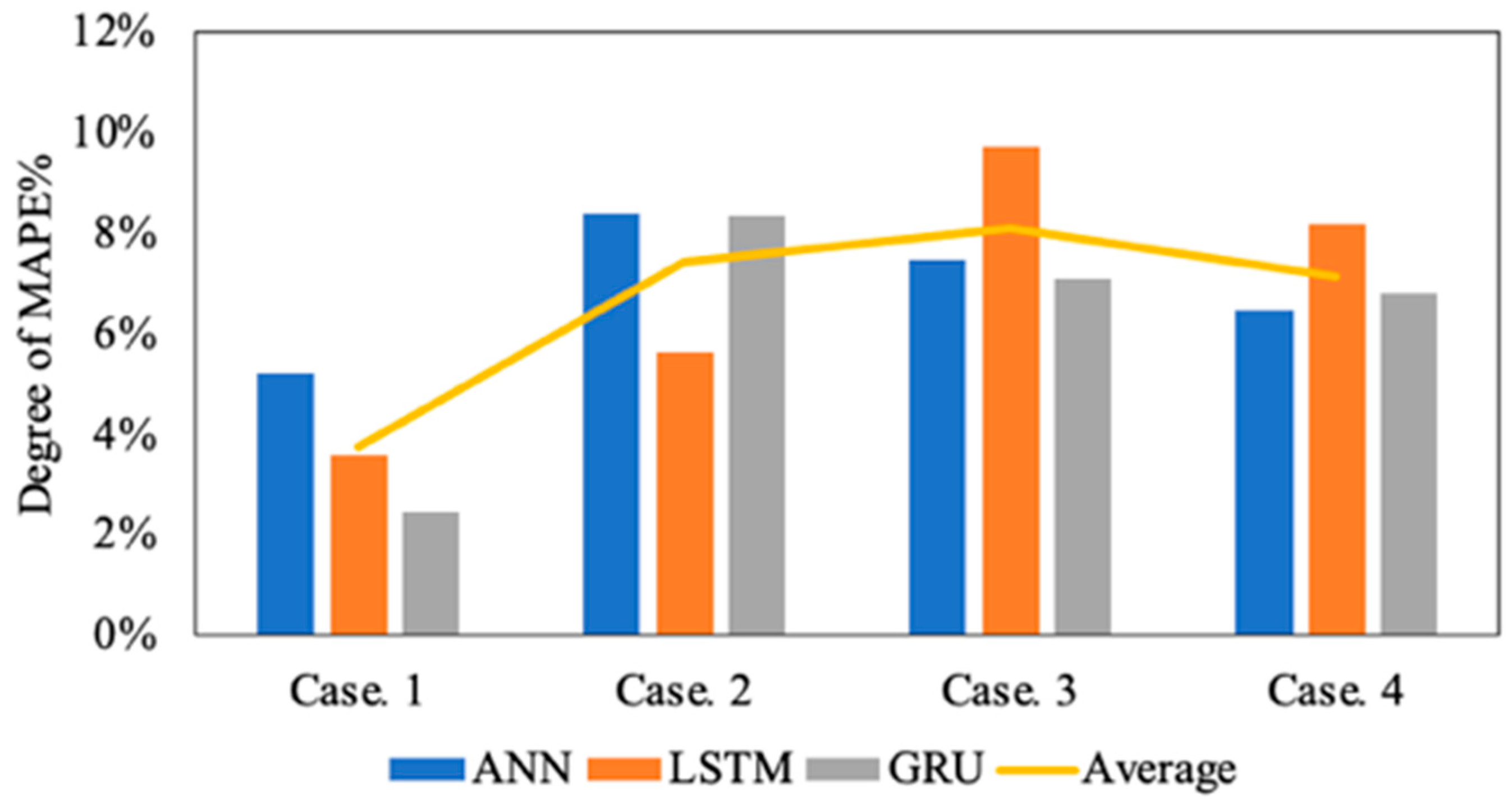
4.4. Performance Comparison with Different Weather Features in One Week

The forecast performance evaluation of the three deep learning models with four cases for one week (from 7 June to 13 June 2021 including sunny, mostly clear, cloudy, and short showers weather) is shown in Figure 10 and

Table 10. The results of the one week PV prediction evaluation.

Index	Model	Case1 1			Case2 2			Case3 3			Case4 4
		MAPE (%)	MAE	RMSE	MAPE (%)	MAE	RMSE	MAPE (%)	MAE	RMSE	MAPE (%)	MAE	RMSE
1	ANN	19.635	0.048	0.095	22.295	0.054	0.106	20.928	0.055	0.102	21.517	0.056	0.114
2	LSTM	16.969	0.048	0.098	18.856	0.054	0.109	24.536	0.058	0.107	20.745	0.061	0.119
3	GRU	16.679	0.049	0.098	18.565	0.529	0.105	17.962	0.057	0.106	18.731	0.056	0.106

¹ Case 1: Six weather values; ² Case 2: Five weather values (without coverage rate); ³ Case 3: Five weather values (without UVI); ⁴ Case 4: Only coverage rate and relatively humidity.

. The results showed that using the six weather features yielded better forecasting accuracy. Among them, 7 June and 8 June were days of short showers. In contrast with the sunny day, adding the cloud coverage rate to the forecast for the PV power showed that the effect was not significant. The main reason for the poor prediction results on rainy days is that the raindrop attaches to the sky imager, which will cause misjudgment when the equation calculates each pixel, resulting in more errors when calculating the coverage rate. This is a shortcoming of the RGB method in calculating the coverage rate. As addressed in the previous section, upon longer prediction period and under more weather conditions, the prediction effect of the GRU model showed better adaptability than that of the LSTM and ANN models. However, the corresponding MAPE was about 16.9%, the MAE was 0.048, and the RMSE was 0.098. On the other hand, from the comparison results, the proposed coverage rate as a weather feature can improve the accuracy by about 2% when compared with the case without coverage rate, meaning that the coverage rate is an imperative feature for short-term PV forecasting.

5. Conclusions

The accuracy of grasping cloud distribution has greatly helped short-term PV power forecasting. The RGB calculation formula and limitation conditions as sky image analysis are proposed in this paper. Furthermore, the authors defined the threshold for obtaining the best coverage rate per minute and as the deep learning model training feature. The novelty of this method is that the calculation is fast and simple. By comparing the one-week forecast results of the four cases, it can be seen that considering all six weather features yielded a complementary effect to improve the forecast accuracy. In particular, adding the cloud coverage rate as a key feature for the PV power forecast increased up to a 2% improvement in accuracy. On the other hand, the result shows that the application of the cloud coverage rate with the deep learning models LSTM and GRU is beneficial to the short-term PV power forecasting. In this regard, adding the cloud coverage rate as a feature parameter to forecast the renewable energy power generation of the microgrid is reliable and robust. In addition, the forecasting result of PV power can also be provided as a reference for the EMS of the regional microgrid to power dispatch.

However, the forecasting result shows that this method is ineffective on rainy days, mainly because the raindrop attaches to the sky imager; the RGB pixels cannot be distinguished. Therefore, the authors will introduce a hybrid model into a micro-grid energy management system for further research. If the weather forecast is specifically a rainy day, a hybrid model will be utilized instead of using the model run by the cloud coverage rate. In contrast, other weather forecast results will be estimated with the model run by the cloud coverage rate.

References

1. Shah, R.; Mithulananthan, N.; Bansal, R.C.; Ramachandaramurthy, V.K. A review of key power system stability challenges for large-scale PV integration. Renew. Sustain. Energy Rev. 2015, 41, 1423–1436. [Google Scholar] [CrossRef]
2. Zhang, Y.; Beaudin, M.; Taheri, R.; Zareipour, H.; Wood, D. Day-ahead power output forecasting for small-scale solar photovoltaic electricity generators. IEEE Trans. Smart Grid 2015, 6, 2253–2262. [Google Scholar] [CrossRef]
3. Verma, T.; Tiwana, A.; Reddy, C.; Arora, V.; Devanand, P. Data Analysis to Generate Models Based on Neural Network and Regression for Solar Power Generation Forecasting. In Proceedings of the 2016 7th International Conference on Intelligent Systems, Modelling and Simulation (ISMS), Bangkok, Thailand, 25–27 January 2016; IEEE: New York, NY, USA, 2016; pp. 97–100. [Google Scholar]
4. Alluhaidah, B.M.; Shehadeh, S.; El-Hawary, M. Most Influential Variables for Solar Radiation Forecasting Using Artificial Neural Networks. In Proceedings of the 2014 IEEE Electrical Power and Energy Conference, Toronto, ON, Canada, 10–11 October 2014; IEEE: New York, NY, USA, 2014; pp. 71–75. [Google Scholar]
5. Nitisanon, S.; Hoonchareon, N. Solar Power Forecast with Weather Classification Using Self-Organized Map. In Proceedings of the 2017 IEEE Power & Energy Society General Meeting, Chicago, IL, USA, 16–20 July 2017; IEEE: New York, NY, USA, 2017; pp. 1–5. [Google Scholar]
6. Agoua, X.G.; Girard, R.; Kariniotakis, G. Short-term spatio-temporal forecasting of photovoltaic power production. IEEE Trans. Sustain. Energy 2017, 9, 538–546. [Google Scholar] [CrossRef] [Green Version]
7. Suksamosorn, S.; Hoonchareon, N.; Songsiri, J. Influential Variable Selection for Improving Solar Forecasts from Numerical Weather Prediction. In Proceedings of the 2018 15th International Conference on Electrical Engineering/Electronics, Computer, Telecommunications and Information Technology (ECTI-CON), Chiang Rai, Thailand, 18–21 July 2018; IEEE: New York, NY, USA, 2018; pp. 333–336. [Google Scholar]
8. Ghonima, M.; Urquhart, B.; Chow, C.; Shields, J.; Cazorla, A.; Kleissl, J. A method for cloud detection and opacity classification based on ground based sky imagery. Atmos. Meas. Tech. 2012, 5, 2881–2892. [Google Scholar] [CrossRef] [Green Version]
9. Shields, J.E.; Karr, M.E.; Burden, A.R.; Johnson, R.W.; Mikuls, V.W.; Streeter, J.R.; Hodgkiss, W.S. Research toward Multi-Site Characterization of Sky Obscuration by Clouds; Scripps Institution of Oceanography La Jolla Ca Marine Physical Lab: La Jolla, CA, USA, 2009. [Google Scholar]
10. Ghanbarzadeh, A.; Noghrehabadi, A.; Assareh, E.; Behrang, M. Solar Radiation Forecasting Based on Meteorological Data Using Artificial Neural Networks. In Proceedings of the 2009 7th IEEE International Conference on Industrial Informatics, Cardiff, UK, 23–36 June 2009; IEEE: New York, NY, USA, 2009; pp. 227–231. [Google Scholar]
11. Pawar, P.; Cortés, C.; Murray, K.; Kleissl, J. Detecting clear sky images. Sol. Energy 2019, 183, 50–56. [Google Scholar] [CrossRef]
12. Zhao, X.; Wei, H.; Wang, H.; Zhu, T.; Zhang, K. 3D-CNN-based feature extraction of ground-based cloud images for direct normal irradiance prediction. Sol. Energy 2019, 181, 510–518. [Google Scholar] [CrossRef]
13. Mammoli, A.; Terren-Serrano, G.; Menicucci, A.; Caudell, T.P.; Martínez-Ramón, M. An experimental method to merge far-field images from multiple longwave infrared sensors for short-term solar forecasting. Sol. Energy 2019, 187, 254–260. [Google Scholar] [CrossRef]
14. Kamadinata, J.O.; Ken, T.L.; Suwa, T. Sky image-based solar irradiance prediction methodologies using artificial neural networks. Renew. Energy 2019, 134, 837–845. [Google Scholar] [CrossRef]
15. Quesada-Ruiz, S.; Chu, Y.; Tovar-Pescador, J.; Pedro, H.; Coimbra, C. Cloud-tracking methodology for intra-hour DNI forecasting. Sol. Energy 2014, 102, 267–275. [Google Scholar] [CrossRef]
16. Zhang, J.; Verschae, R.; Nobuhara, S.; Lalonde, J.-F. Deep photovoltaic nowcasting. Sol. Energy 2018, 176, 267–276. [Google Scholar] [CrossRef] [Green Version]
17. Kong, W.; Jia, Y.; Dong, Z.Y.; Meng, K.; Chai, S. Hybrid approaches based on deep whole-sky-image learning to photovoltaic generation forecasting. Appl. Energy 2020, 280, 115875. [Google Scholar] [CrossRef]
18. Wang, F.; Zhang, Z.; Chai, H.; Yu, Y.; Lu, X.; Wang, T.; Lin, Y. Deep Learning Based Irradiance Mapping Model for Solar PV Power Forecasting Using Sky Image. In Proceedings of the 2019 IEEE Industry Applications Society Annual Meeting, Baltimore, MD, USA, 29 September–3 October 2019; IEEE: New York, NY, USA, 2019; pp. 1–9. [Google Scholar]
19. Zhen, Z.; Liu, J.; Zhang, Z.; Wang, F.; Chai, H.; Yu, Y.; Lu, X.; Wang, T.; Lin, Y. Deep learning based surface irradiance mapping model for solar PV power forecasting using sky image. IEEE Trans. Ind. Appl. 2020, 56, 3385–3396. [Google Scholar] [CrossRef]
20. Wen, H.; Du, Y.; Chen, X.; Lim, E.; Wen, H.; Jiang, L.; Xiang, W. Deep learning based multistep solar forecasting for PV ramp-rate control using sky images. IEEE Trans. Ind. Inform. 2020, 17, 1397–1406. [Google Scholar] [CrossRef]
21. Srivastava, N.; Hinton, G.; Krizhevsky, A.; Sutskever, I.; Salakhutdinov, R. Dropout: A simple way to prevent neural networks from overfitting. J. Mach. Learn. Res. 2014, 15, 1929–1958. [Google Scholar]
22. Greff, K.; Srivastava, R.K.; Koutník, J.; Steunebrink, B.R.; Schmidhuber, J. LSTM: A search space odyssey. IEEE Trans. Neural Netw. Learn. Syst. 2016, 28, 2222–2232. [Google Scholar] [CrossRef] [PubMed] [Green Version]
23. Cho, K.; Van Merriënboer, B.; Gulcehre, C.; Bahdanau, D.; Bougares, F.; Schwenk, H.; Bengio, Y. Learning phrase representations using RNN encoder-decoder for statistical machine translation. arXiv 2014, arXiv:1406.1078. [Google Scholar]
24. Chen, Z.; Yang, Y. Assessing forecast accuracy measures. Prepr. Ser. 2004, 2010, 2004–2010. [Google Scholar]
Figure 1. The PV power forecasting procedures, introducing Data Collection, Data Preprocessing, Model Building & Training, and Forecasting Processes.
Energies 15 04779 g001
Figure 2. The use of the equipment (PV inverter, Weather Station, Whole Sky Imagers) and data collection schema (using Modbus TCP/IP).
Energies 15 04779 g002
Figure 3. The results of the average distribution of each element.
Energies 15 04779 g003
Figure 4. The cloud covering process.
Energies 15 04779 g004
Figure 5. Case 1—(a) Forecasting results of 16 March 2021(sunny). (b) Forecasting results of 21 May 2021(mostly cloudy). The frequency of data collection was once per minute.
Energies 15 04779 g005
Figure 6. Case 2—(a) Forecasting results of 16 March 2021 (sunny). (b) Forecasting results of 21 May 2021 (mostly cloudy). The frequency of data collection was once per minute.
Energies 15 04779 g006
Figure 7. Case 3—(a) Forecasting results of 16 March 2021 (sunny). (b) Forecasting results of 21 May 2021 (mostly cloudy). The frequency of data collection was once per minute.
Energies 15 04779 g007
Figure 8. Case 4—(a) Forecasting results of 16 March 2021 (sunny). (b) Forecasting results of 21 May 2021 (mostly cloudy). The frequency of data collection was once per minute.
Energies 15 04779 g008
Figure 9. The comprehensive analysis and average degree of the MAPE change with different weather feature combinations.
Energies 15 04779 g009
Figure 10. The forecasting results of the four cases from 7 June to 13 June 2021. The frequency of data collection was once per minute. (a) One week forecasting results of Case 1 (six weather values). (b) One week forecasting results of Case 2 (five weather values (without coverage rate)). (c) One week forecasting results of Case 3 (five weather values (without UVI)). (d) One week forecasting results of Case 4 (only coverage rate and relatively humidity).
Energies 15 04779 g010aEnergies 15 04779 g010b